
Canopy Gap Mapping from Airborne Laser Scanning: An Assessment of the Positional and Geometrical Accuracy


Abstract
:
1. Introduction
1.1. Canopy Gap Mapping with ALS : A Background
1.2. Aims of the Study
2. Data Sets
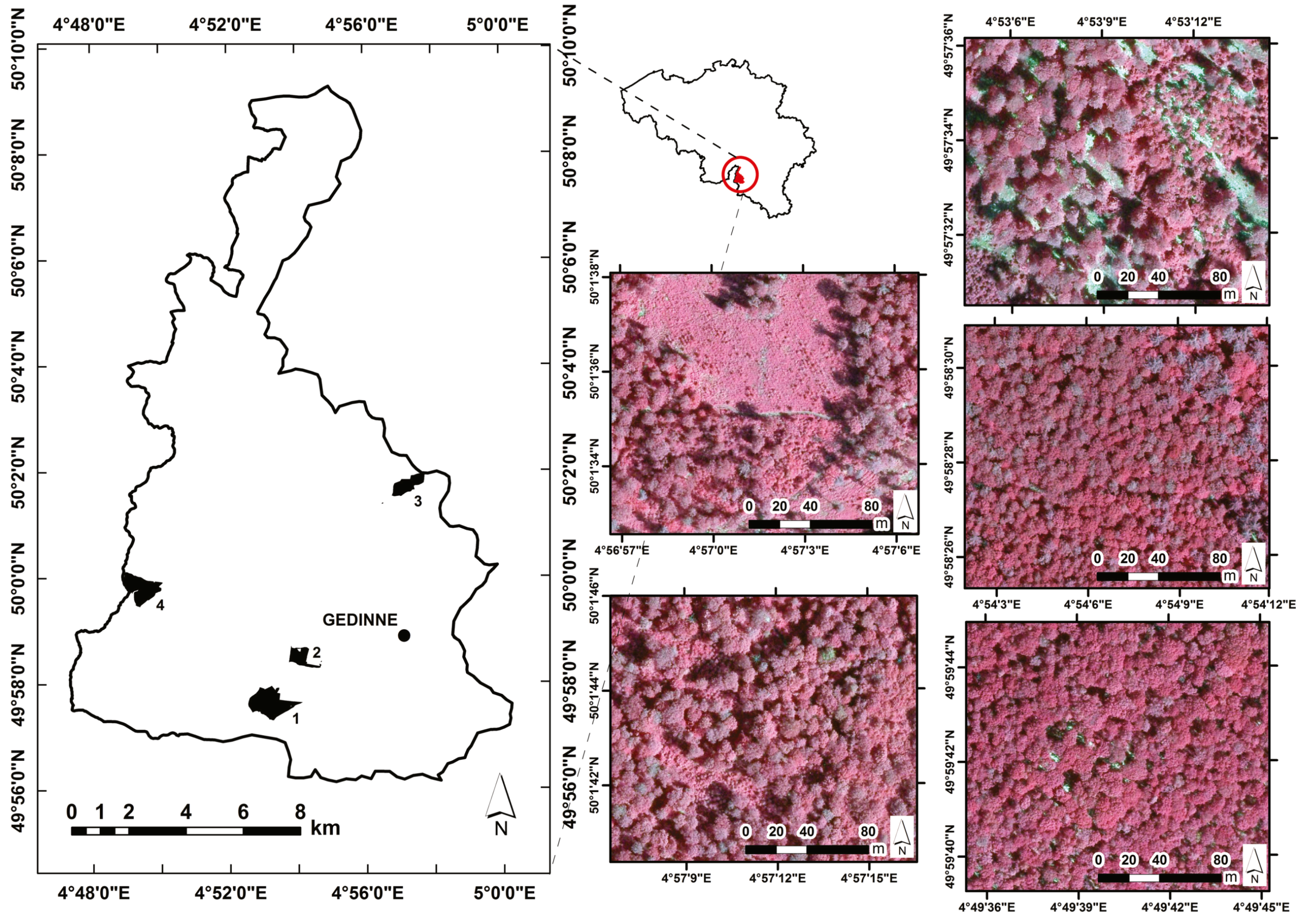
2.1. Study Site

2.2. Canopy Gap Definition
2.3. Field Data
2.4. ALS Data
2.5. Pre-Processing of ALS Data

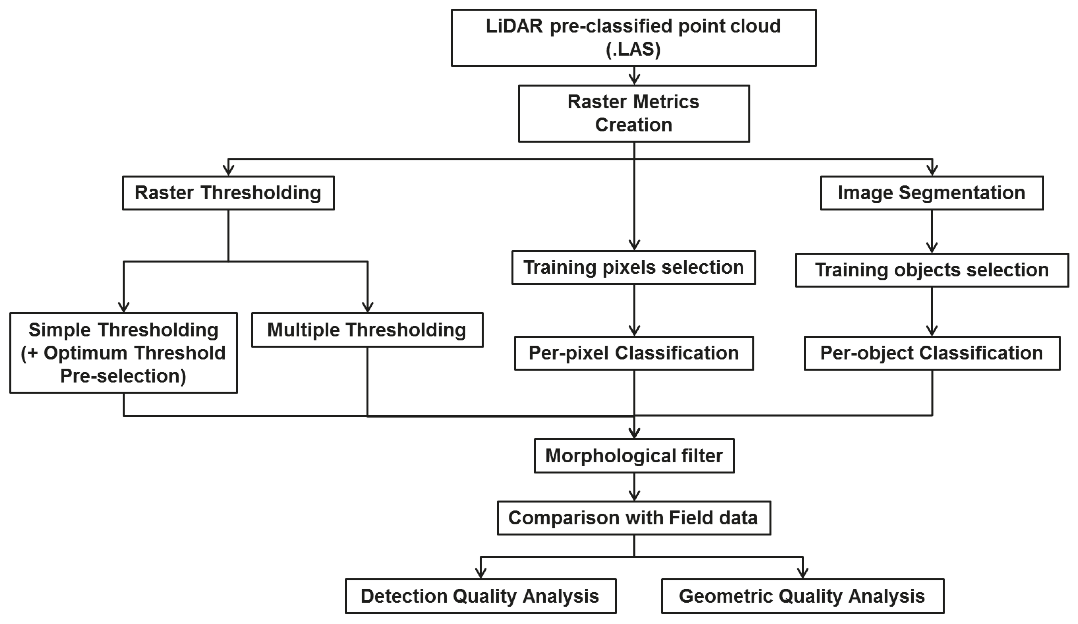
3. Methodology
3.1. Gap Mapping Methods

3.1.1. Thresholding
- CHM: gaps are identified as grid cells with a height below 3 m or 5 m;
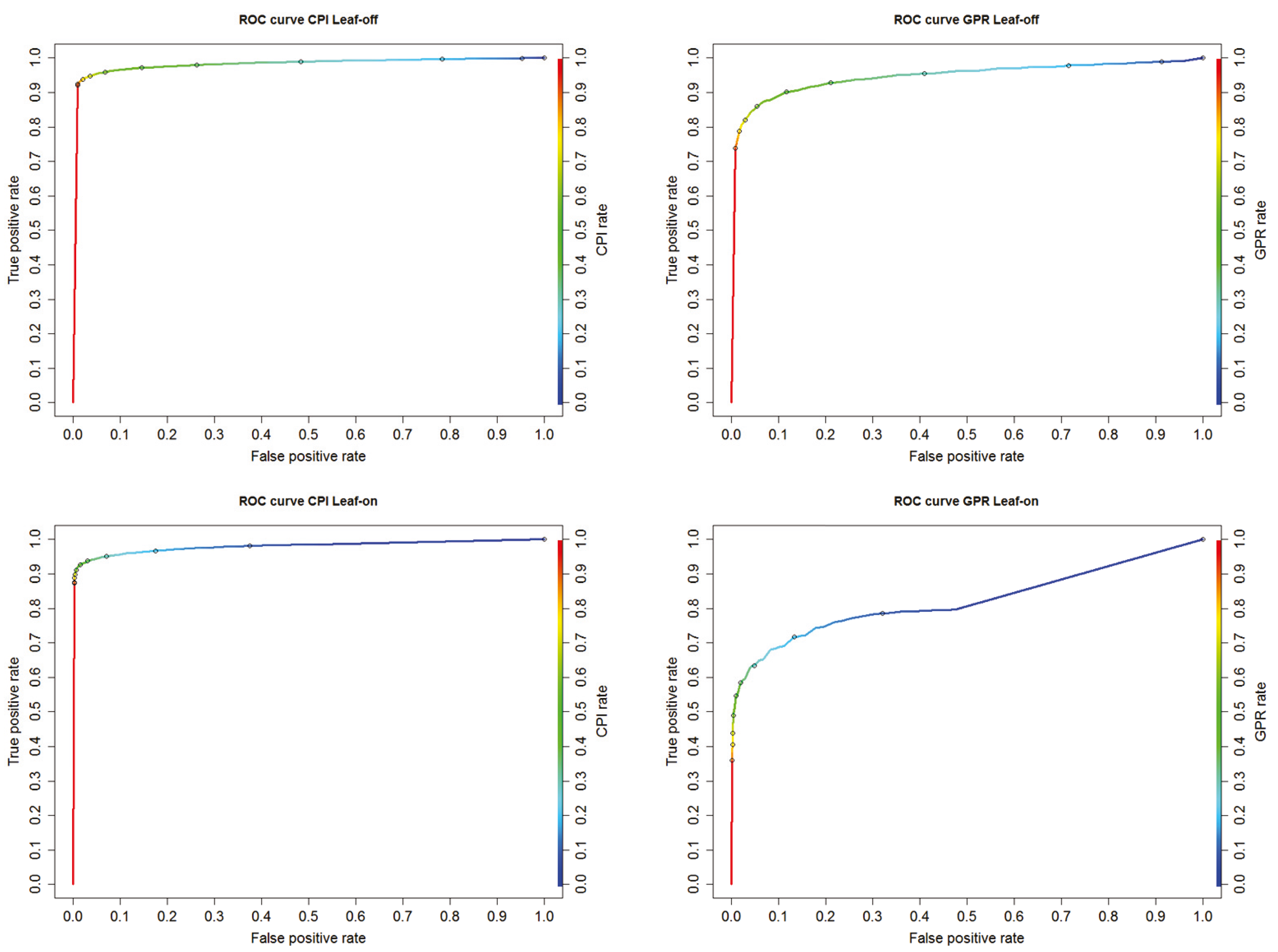
- CPI and GPR: gaps are identified as grid cells with a CPI/GPR above a threshold. A specific step to determine the optimum threshold values for CPI and GPR (respectively for leaf-off and leaf-on) was implemented to avoid a systematic test of several values for each datasets. This threshold selection is presented in Section 3.2.1.
- Combination1: CHM-3m + CPI-75% +Slope-H-75%
- Combination2: CHM-5m + CPI-55% +Slope-H-60%
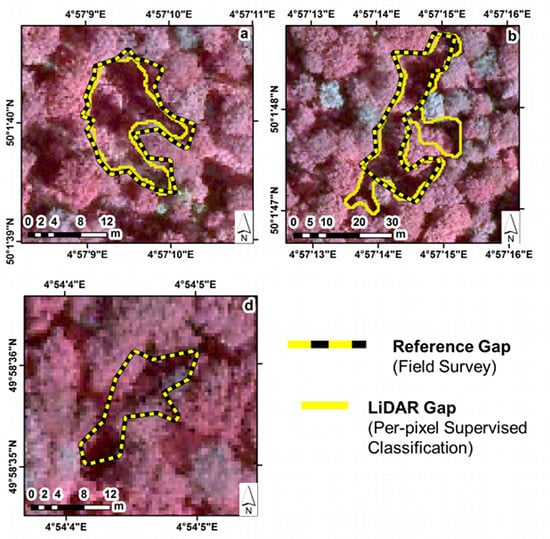
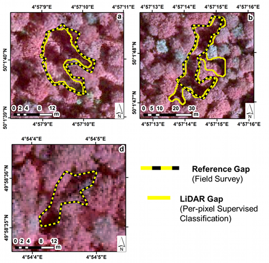
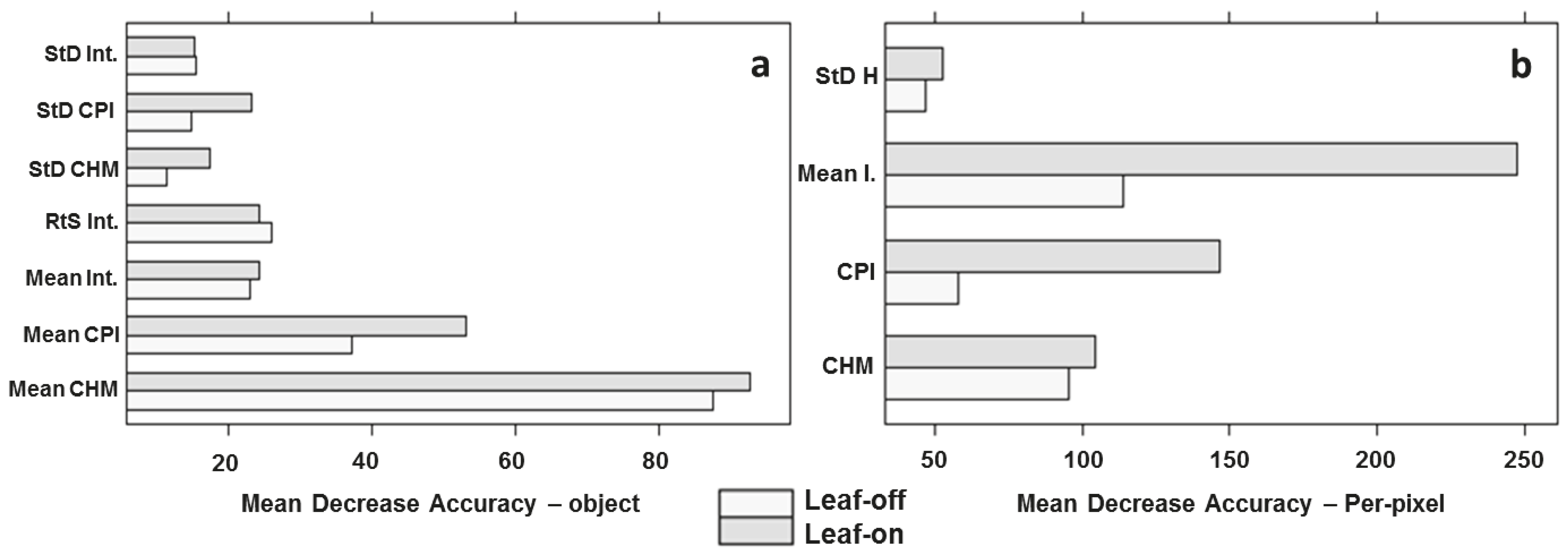
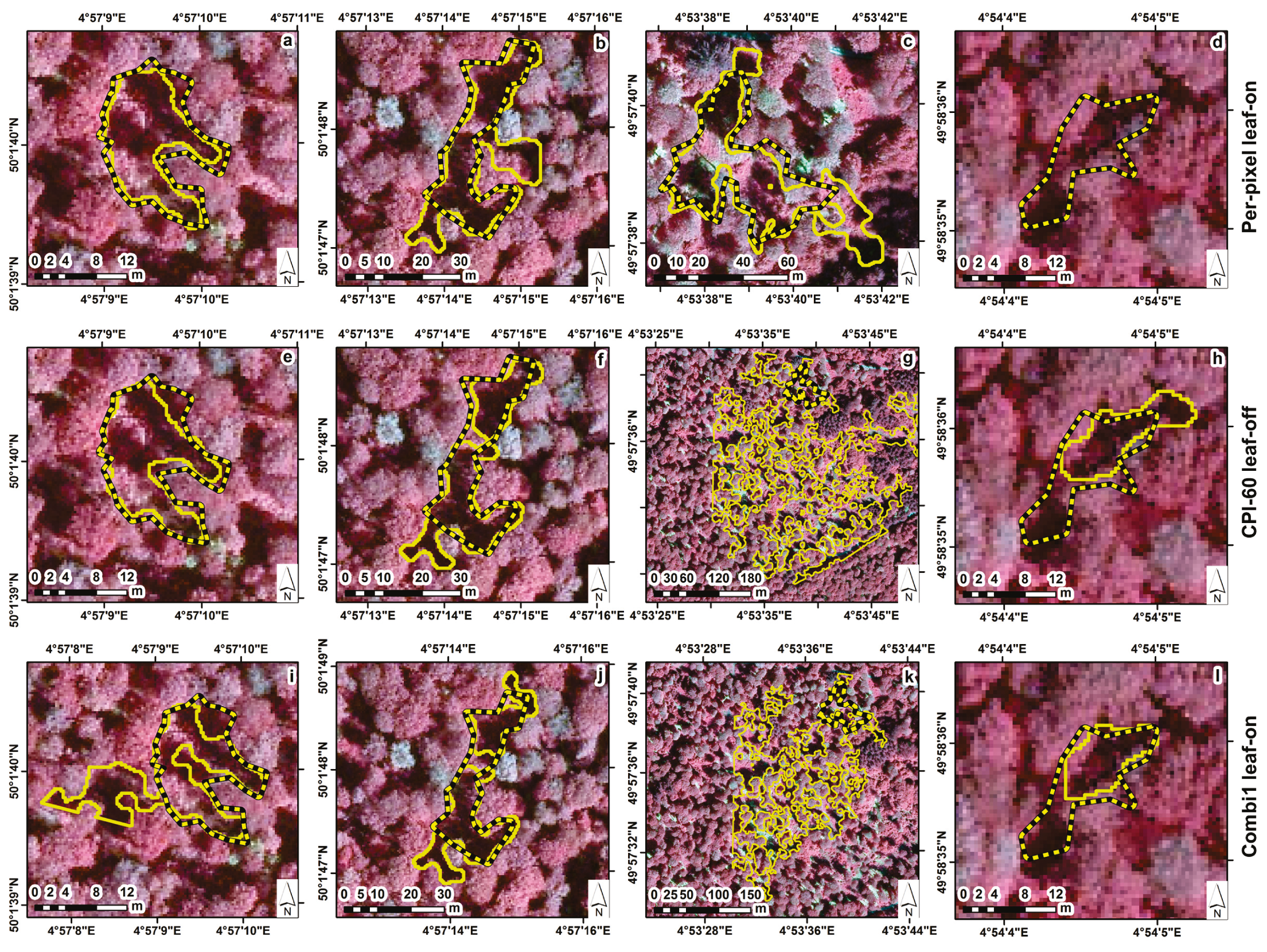
3.1.2. Per-Pixel Supervised Classification
3.1.3. Per-Object Supervised Classification
3.1.4. Morphological Filtering
3.2. Analysis of Mapping Quality
3.2.1. Gap Detection
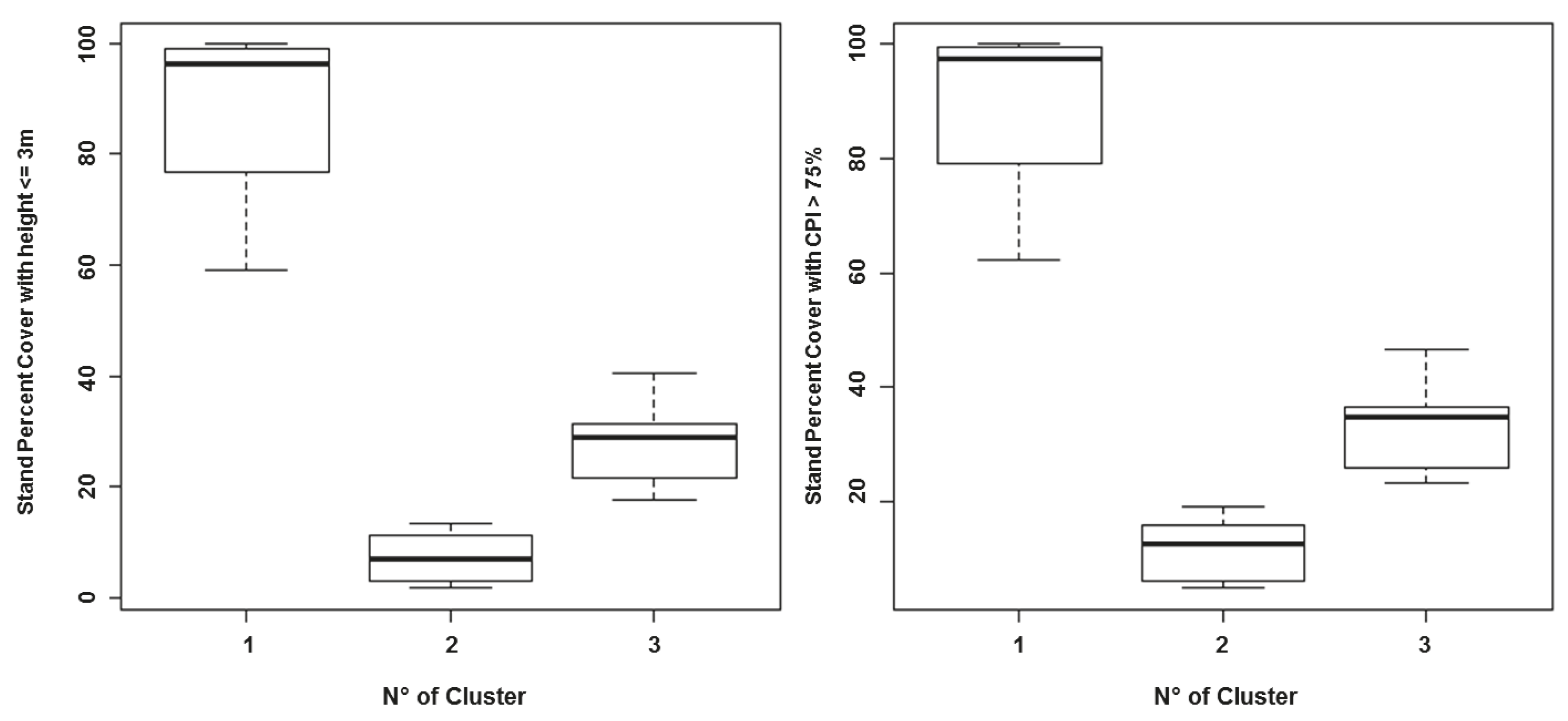
3.2.2. Influence of Stand Type on Gap Detection
3.2.3. Gaps Geometry
- Gap Shape Complexity Index [21]GSCI is a measure of the relative complexity of shape; it compares the shape of the gap to a circle. It is computed as the ratio of a gap’s perimeter to the perimeter of a circular gap of the same area. An increasing value of GSCI is an increasing shape complexity [13,21].
- Area of the gap ( m2)
- Main direction (degrees): This is the azimuth of the longest line within the boundaries of the polygon without crossing edges. This line is created by the geom.polygonfetch command of Geospatial Modelling Environment. The azimuth value ranges between 0 and 180 degrees.
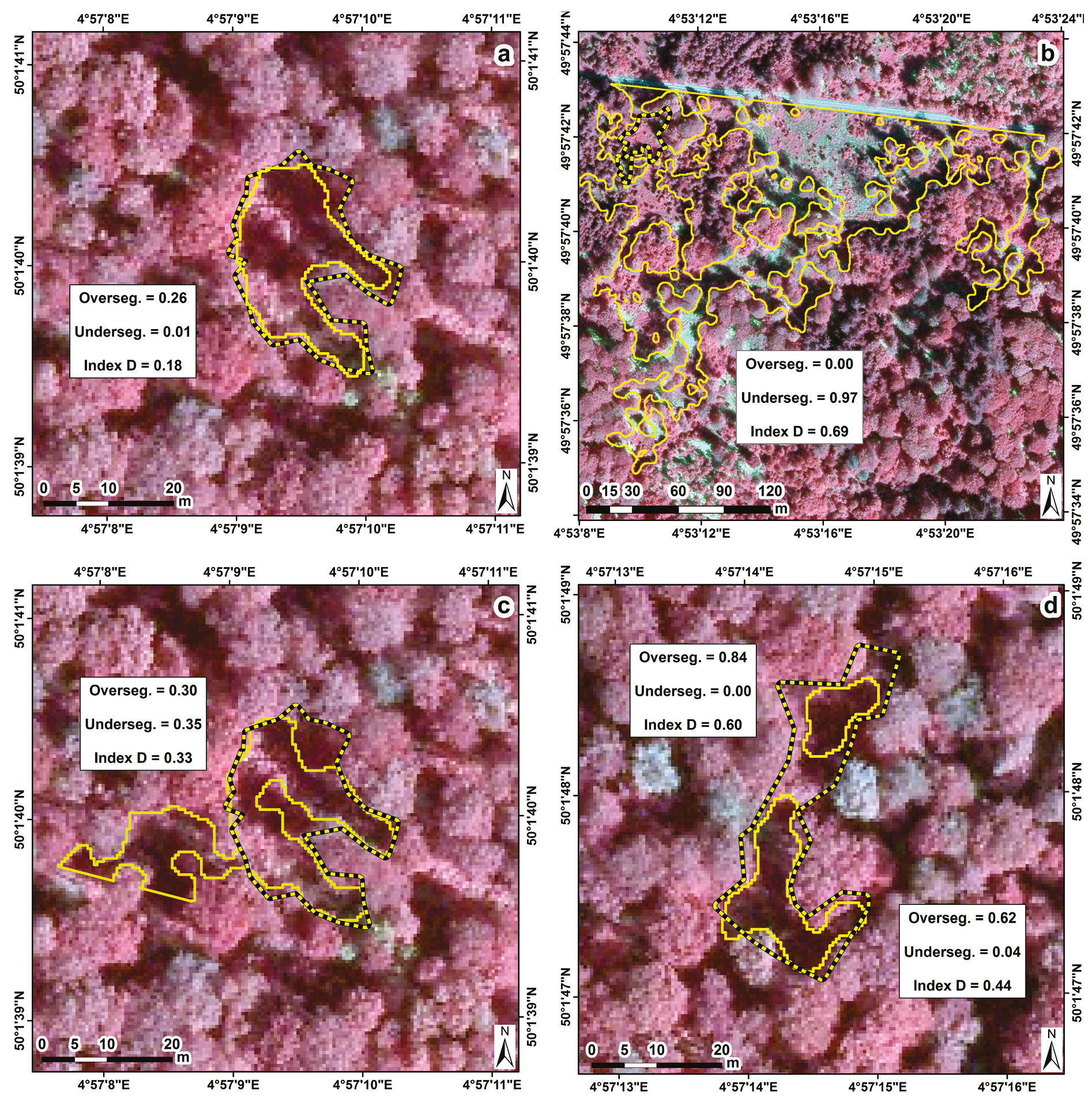
- Index D: derived from Oversegmentation and Undersegmentation (Equations (2) to (4)). This index is used in several studies to assess the accuracy of object-based image segmentation [43,44], to determine best segmentation parameters. Index D is a distance which varies between 0–1 and is a quantitative assessment of the goodness of polygon matching. Index D has to be minimized and a good balance between oversegmentation and undersegmentation has to be found to optimize the results. In this analysis, polygons for which the ratio of the intersected area between ALS and field gaps was a minimum 10% were retained (compared to 50% in Möller et al. [43] and Clinton et al. [44]).
4. Results
4.1. Gaps Detection Accuracy
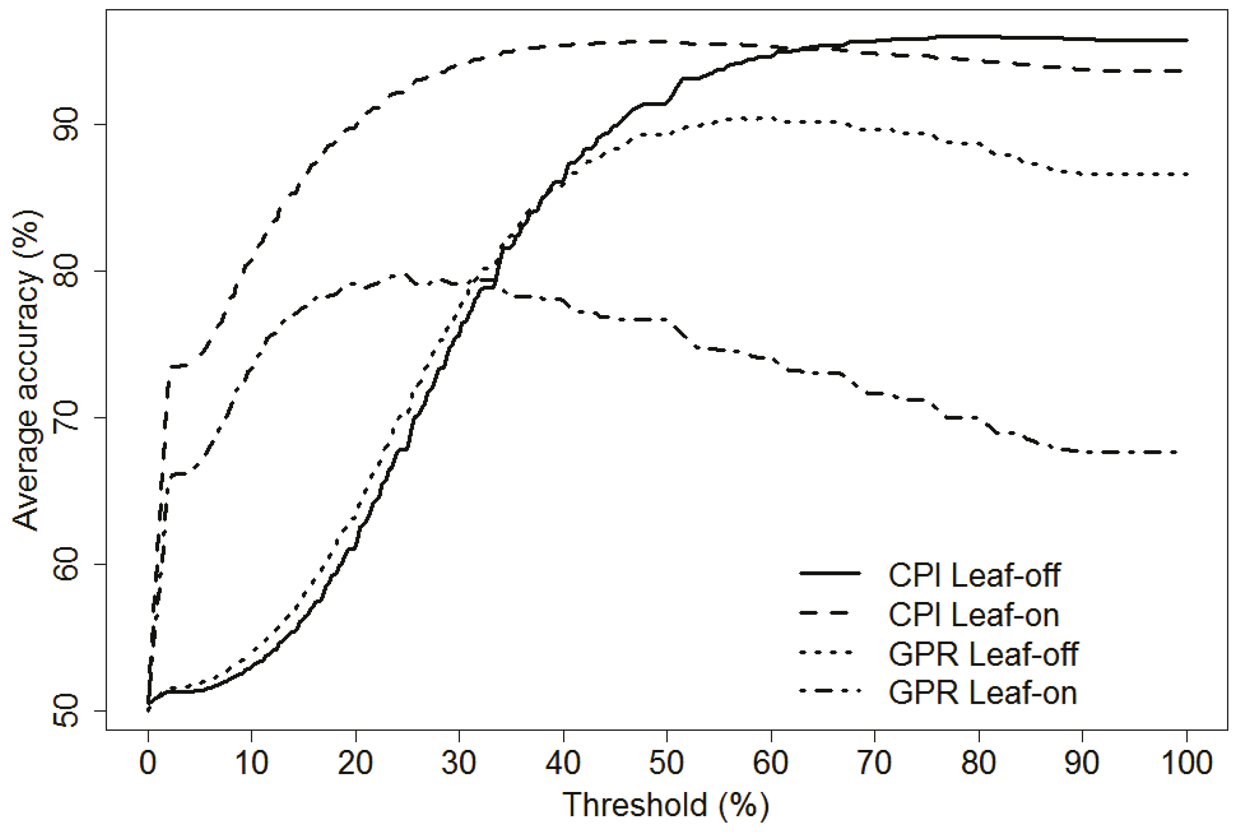
4.1.1. Optimum Threshold Selection for CPI and GPR
4.1.2. Summary of the Confusion Matrices


| Leaf-off | Leaf-on | |||||
|---|---|---|---|---|---|---|
| Type | GA | PA | CA | GA | PA | CA |
| Simple threshold. | ||||||
| CHM-3m | 0.78 | 0.60 | 0.93 | 0.72 | 0.50 | 0.90 |
| CHM-5m | 0.81 | 0.66 | 0.93 | 0.77 | 0.60 | 0.91 |
| CPI-50 | 0.78 | 0.63 | 0.91 | |||
| CPI-60 | 0.82 | 0.73 | 0.88 | |||
| GPR-60 | 0.76 | 0.52 | 0.89 | |||
| Multiple threshold. | ||||||
| Combination1 | 0.79 | 0.81 | 0.78 | 0.80 | 0.71 | 0.87 |
| Combination2 | 0.62 | 0.94 | 0.58 | 0.73 | 0.86 | 0.68 |
| Superv. classif. | ||||||
| Per-pixel | 0.81 | 0.73 | 0.88 | 0.81 | 0.73 | 0.90 |
| Per-object | 0.79 | 0.77 | 0.81 | 0.80 | 0.72 | 0.86 |
| Per-Object | Per-Pixel | ||
|---|---|---|---|
| Leaf-off | Leaf-on | Leaf-off | Leaf-on |
| 98.1% | 96.3% | 97.0% | 97.2% |
4.1.3. Leaf-on vs. Leaf-off

4.1.4. Thresholding vs. Supervised Classification
4.1.5. Per-Object vs. Per-Pixel
4.1.6. CHM Thresholding vs. other Metrics
| Per-Pixel | CPI-60 | Combination1 | |
|---|---|---|---|
| Leaf-on | Leaf-off | Leaf-on | |
| Global accuracy | 4% | 1% | 3% |
| Producer accuracy | 13% | 7% | 11% |
| Consumer accuracy | –1% | –5% | –4% |
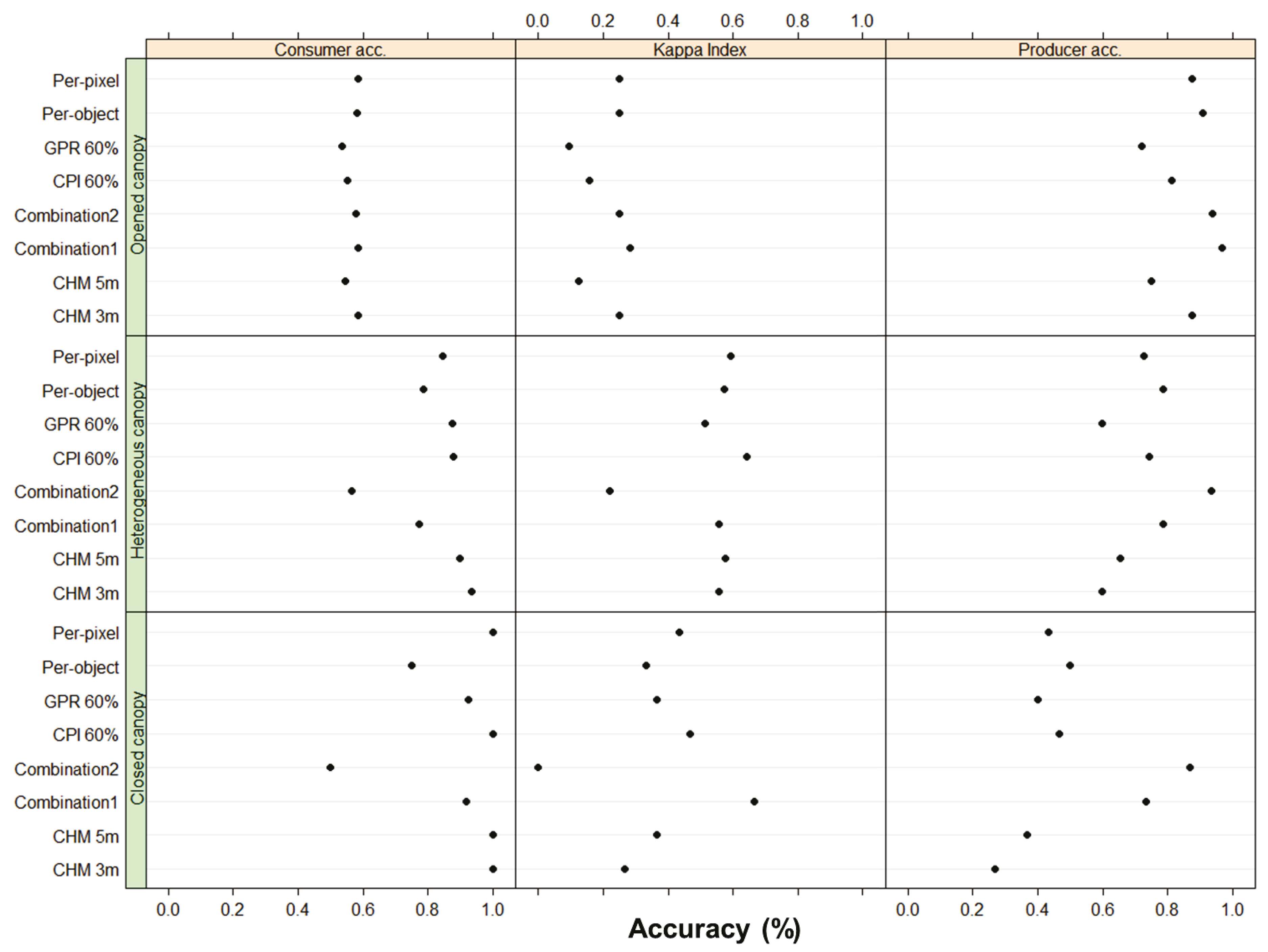
4.2. Influence of Stand Type on Gap Detection


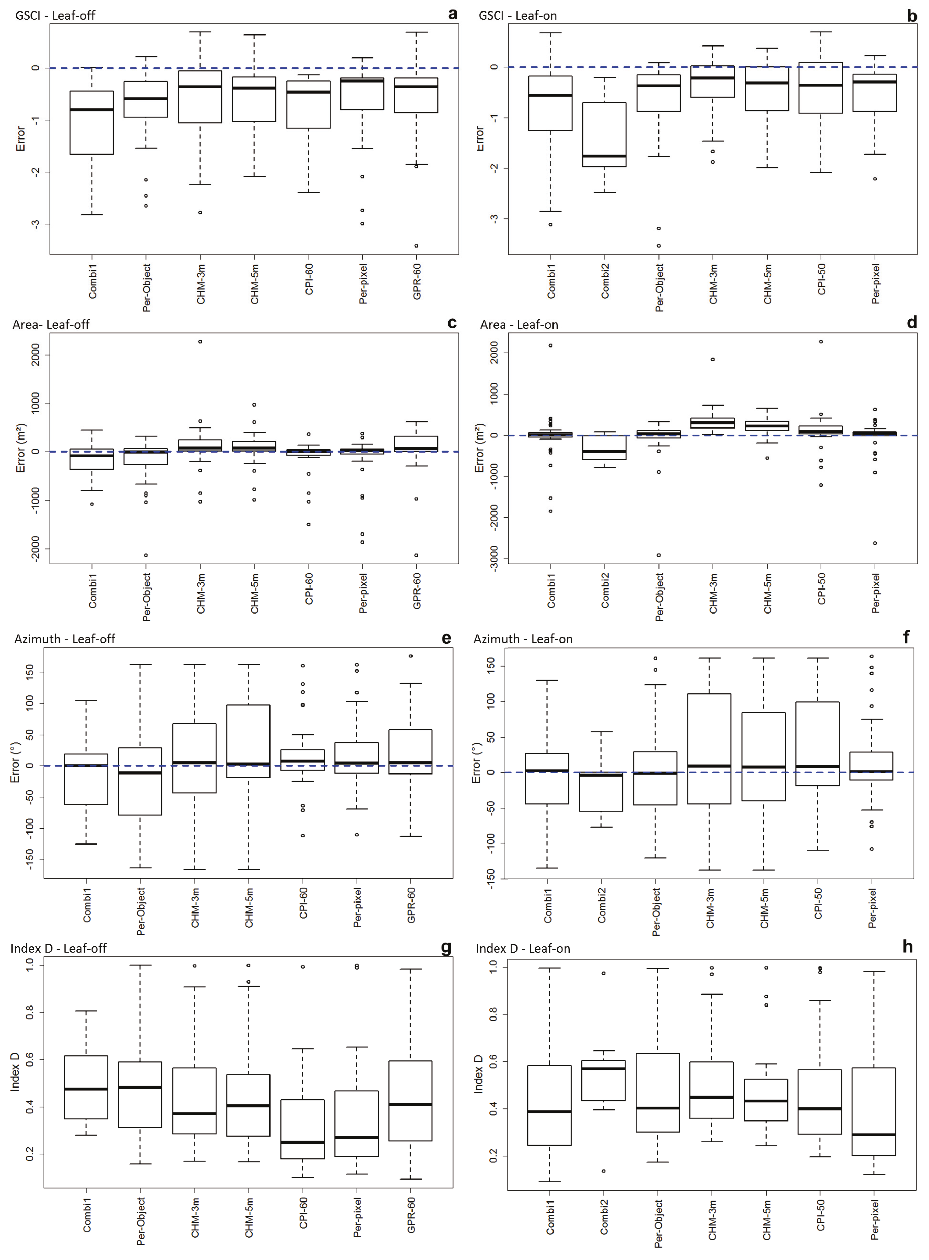
4.3. Gaps Geometry Accuracy
4.3.1. GSCI
4.3.2. Gap Area
4.3.3. Main Direction


4.3.4. Index D

5. Discussion
6. Conclusions
Acknowledgments
Author Contributions
Conflicts of Interest
References
- Degen, T.; Devillez, F.; Jacquemart, A.L. Gaps promote plant diversity in beech forests (Luzulo–Fagetum), North Vosges, France. Ann. For. Sci. 2005, 62, 429–440. [Google Scholar] [CrossRef]
- Dobrowolska, D.; Veblen, T. Treefall—Gap structure and regeneration in mixed Abies alba stands in central Poland. For. Ecol. Manag. 2008, 255, 3469–3476. [Google Scholar] [CrossRef]
- Schliemann, S.; Bockheim, J. Methods for studying treefall gaps: A review. For. Ecol. Manag. 2011, 261, 1143–1151. [Google Scholar] [CrossRef]
- Blackburn, G.A.; Milton, E. Filling the gaps: Remote sensing meets woodland ecology. Glob. Ecol. Biogeogr. Lett. 1996, 5, 175–191. [Google Scholar] [CrossRef]
- Kane, V.R.; Gersonde, R.F.; Lutz, J.A.; McGaughey, R.J.; Bakker, J.D.; Franklin, J.F. Patch dynamics and the development of structural and spatial heterogeneity in pacific northwest forests. Can. J. For. Res. 2011, 41, 2276–2291. [Google Scholar] [CrossRef]
- Malcolm, D.; Mason, W.; Clarke, G. The transformation of conifer forests in Britain-regeneration, gap size and silvicultural systems. For. Ecol. Manag. 2001, 151, 7–23. [Google Scholar] [CrossRef]
- Runkle, J.R. Patterns of disturbance in some old–growth mesic forests of eastern North America. Ecology 1982, 63, 1533–1546. [Google Scholar] [CrossRef]
- Vehmas, M.; Packalen, P.; Maltamo, M.; Eerikainen, K. Using airborne laser scanning data for detecting canopy gaps and their understory type in mature boreal forest. Ann. For. Sci. 2011, 68, 825–835. [Google Scholar] [CrossRef]
- Watt, A.S. Pattern and process in the plant community. J. Ecol. 1947, 35, 1–22. [Google Scholar] [CrossRef]
- Koukoulas, S.; Blackburn, G. Spatial relationships between tree species and gap characteristics in broad–leaved deciduous woodland. J. Veg. Sci. 2005, 16, 587–596. [Google Scholar] [CrossRef]
- Lindenmayer, D.; Franklin, J.; Fischer, J. General management principles and a checklist of strategies to guide forest biodiversity conservation. Biol. Conserv. 2006, 131, 433–445. [Google Scholar] [CrossRef]
- Poulson, T.L.; Platt, W.J. Gap light regimes influence canopy tree diversity. Ecology 1989, 70, 553–555. [Google Scholar] [CrossRef]
- Getzin, S.; Wiegand, K.; Schöning, I. Assessing biodiversity in forests using very high-resolution images and unmanned aerial vehicles. Methods Ecol. Evol. 2012, 3, 397–404. [Google Scholar] [CrossRef]
- Betts, H.; Brown, L.; Stewart, G. Forest canopy gap detection and characterisation by the use of high–resolution digital eevation models. N. Zeal. J. Ecol. 2005, 29, 95–103. [Google Scholar]
- Yamamoto, S.; Nishimura, N.; Torimaru, T.; Manabe, T.; Itaya, A.; Becek, K. A comparison of different survey methods for assessing gap parameters in old–growth forests. For. Ecol. Manag. 2011, 262, 886–893. [Google Scholar] [CrossRef]
- Vepakomma, U.; St-Onge, B.; Kneeshaw, D. Spatially explicit characterization of boreal forest gap dynamics using multi–temporal lidar data. Remote Sens. Environ. 2008, 112, 2326–2340. [Google Scholar] [CrossRef]
- Brokaw, N.V. The definition of treefall gap and its effect on measures of forest dynamics. Biotropica 1982, 14, 158–160. [Google Scholar] [CrossRef]
- Gaulton, R.; Malthus, T.J. LiDAR mapping of canopy gaps in continuous cover forests: A comparison of canopy height model and point cloud based techniques. Int. J. Remote Sens. 2010, 31, 1193–1211. [Google Scholar] [CrossRef]
- Asner, G.P.; Kellner, J.R.; Kennedy-Bowdoin, T.; Knapp, D.E.; Anderson, C.; Martin, R.E. Forest canopy gap distributions in the Southern Peruvian Amazon. PLoS ONE 2013, 8, e60875. [Google Scholar] [CrossRef] [PubMed]
- Boyd, D.S.; Hill, R.A.; Hopkinson, C.; Baker, T.R. Landscape–scale forest disturbance regimes in Southern Peruvian Amazonia. Ecol. Appl. 2013, 23, 1588–1602. [Google Scholar] [CrossRef]
- Koukoulas, S.; Blackburn, G. Quantifying the spatial properties of forest canopy gaps using LiDAR imagery and GIS. Int. J. Remote Sens. 2004, 25, 3049–3072. [Google Scholar] [CrossRef]
- Zhang, K. Identification of gaps in mangrove forests with airborne LiDAR. Remote Sens. Environ. 2008, 112, 2309–2325. [Google Scholar] [CrossRef]
- Korhonen, L.; Korhonen, K.T.; Rautiainen, M.; Stenberg, P. Estimation of forest canopy cover: A comparison of field measurement techniques. Silva Fenn. 2006, 40, 577–588. [Google Scholar] [CrossRef]
- Korhonen, L.; Korpela, I.; Heiskanen, J.; Maltamo, M. Airborne discrete-return LiDAR data in the estimation of vertical canopy cover, angular canopy closure and leaf area index. Remote Sens. Environ. 2011, 115, 1065–1080. [Google Scholar] [CrossRef]
- Korhonen, L.; Morsdorf, F. Estimation of canopy cover, gap fraction and leaf area index with airborne laser scanning. In Forestry Applications of Airborne Laser Scanning: Concepts and Case Studies; Maltamo, M., Næsset, E., Vauhkonen, J., Eds.; Springer Science & Business Media: Dordrecht, The Netherlands, 2014; Volume 27, pp. 397–417. [Google Scholar]
- Jennings, S.; Brown, N.; Sheil, D. Assessing forest canopies and understorey illumination: Canopy closure, canopy cover and other measures. Forestry 1999, 72, 59–74. [Google Scholar] [CrossRef]
- Saint-Onge, B.; Vepakomma, U.; Sénécal, J.F.; Kneeshaw, D.; Doyon, F. Canopy gap dectection and analysis with airborne laser scanning. In Forestry Applications of Airborne Laser Scanning: Concepts and Case Studies; Maltamo, M., Næsset, E., Vauhkonen, J., Eds.; Springer Science & Business Media: Dordrecht, The Netherlands, 2014; Volume 27, pp. 419–438. [Google Scholar]
- Breiman, L. Random forests. Mach. Learn. 2001, 45, 5–32. [Google Scholar] [CrossRef]
- Ligot, G.; Balandier, P.; Fayolle, A.; Lejeune, P.; Claessens, H. Height competition between Quercus Petraea and Fagus Sylvatica natural regeneration in mixed and uneven–aged stands. For. Ecol. Manag. 2013, 304, 391–398. [Google Scholar] [CrossRef]
- Alderweireld, M.; Ligot, G.; Latte, N.; Claessens, H. Le chêne en forêt ardennaise, un atout à préserver. Forêt Wallonne 2010, 109, 10–24. [Google Scholar]
- Bruciamacchie, M.; Grandjean, G.; Jacobée, F. Installation de régénérations feuillues dans de petites trouées en peuplements irréguliers. Revue For. Fr. 1994, 6, 639–652. [Google Scholar] [CrossRef]
- Nagel, T.; Svoboda, M.; Rugani, T.; Diaci, J. Gap regeneration and replacement patterns in an old-growth Fagus–Abies forest of Bosnia–Herzegovina. Plant Ecol. 2010, 208, 307–318. [Google Scholar] [CrossRef]
- Isenburg, M. LAStools—Efficient tools for LiDAR processing (Version 150406, Academic), 2015. Available online: http://rapidlasso.com/LAStools (accessed on 28 August 2015).
- Lee, A.; Lucas, R. A LiDAR–derived canopy density model for tree stem and crown mapping in Australian forests. Remote Sens. Environ. 2007, 111, 493–518. [Google Scholar] [CrossRef]
- Liaw, A.; Wiener, M. Classification and regression by randomForest. R News 2002, 2, 18–22. [Google Scholar]
- R Development Core Team. R: A Language and Environment for Statistical Computing; R Foundation for Statistical Computing: Vienna, Austria, 2015. [Google Scholar]
- Genuer, R.; Poggi, J.M.; Tuleau-Malot, C. Variable selection using Random Forests. Pattern Recognit. Lett. 2010, 31, 2225–2236. [Google Scholar] [CrossRef]
- Baatz, M.; Hoffmann, C.; Willhauck, G. Progressing from object-based to object-oriented image analysis. In Object-Based Image Analysis; Springer: Berlin, Germany, 2008; pp. 29–42. [Google Scholar]
- Benz, U.C.; Hofmann, P.; Willhauck, G.; Lingenfelder, I.; Heynen, M. Multi-resolution, object-oriented fuzzy analysis of remote sensing data for GIS-ready information. ISPRS J. Photogramm. Remote Sens. 2004, 58, 239–258. [Google Scholar] [CrossRef]
- Baatz, M.; Schäpe, A. Multiresolution segmentation—An optimization approach for high quality multi-scale image segmentation. In Angewandte Geographische Informationsverarbeitung XII; Strobl, J., Blaschke, T., Griesebner, G., Eds.; Wichmann: Heidelberg, Germany, 2000; pp. 12–23. [Google Scholar]
- Sing, T.; Sander, O.; Beerenwinkel, N.; Lengauer, T. ROCR: Visualizing classifier performance in R. Bioinformatics 2005, 21, 3940–3941. [Google Scholar] [CrossRef] [PubMed]
- Lillesand, T.; Kiefer, R.W.; Chipman, J. Remote Sensing and Image Interpretation, 6th ed.; John Wiley & Sons: Hoboken, NJ, USA, 2008. [Google Scholar]
- Möller, M.; Lymburner, L.; Volk, M. The comparison index: A tool for assessing the accuracy of image segmentation. Int. J. Appl. Earth Observ. Geoinf. 2007, 9, 311–321. [Google Scholar] [CrossRef]
- Clinton, N.; Holt, A.; Scarborough, J.; Yan, L.; Gong, P. Accuracy assessment measures for object–based image segmentation goodness. Photogramm. Eng. Remote Sens. 2010, 76, 289–299. [Google Scholar] [CrossRef]
- Getzin, S.; Nuske, R.S.; Wiegand, K. Using Unmanned Aerial Vehicles (UAV) to quantify spatial gap patterns in forests. Remote Sens. 2014, 6, 6988–7004. [Google Scholar] [CrossRef]
- Lisein, J.; Pierrot-Deseilligny, M.; Bonnet, S.; Lejeune, P. A photogrammetric workflow for the creation of a forest canopy height model from small unmanned aerial system imagery. Forests 2013, 4, 922–944. [Google Scholar] [CrossRef]
- Hytteborn, H.; Verwijst, T. Small-scale disturbance and stand structure dynamics in an old-growth Picea abies forest over 54 year in central Sweden. J. Veg. Sci. 2014, 25, 100–112. [Google Scholar] [CrossRef]
- Blackburn, G.A.; Abd Latif, Z.; Boyd, D.S. Forest disturbance and regeneration: A mosaic of discrete gap dynamics and open matrix regimes? J. Veg. Sci. 2014, 25, 1341–1354. [Google Scholar] [CrossRef]
- Vepakomma, U.; Kneeshaw, D.; st-Onge, B. Interactions of multiple disturbances in shaping boreal forest dynamics: A spatially explicit analysis using multi–temporal lidar data and high–resolution imagery. J. Ecol. 2010, 98, 526–539. [Google Scholar] [CrossRef]
© 2015 by the authors; licensee MDPI, Basel, Switzerland. This article is an open access article distributed under the terms and conditions of the Creative Commons Attribution license (http://creativecommons.org/licenses/by/4.0/).
Share and Cite
Bonnet, S.; Gaulton, R.; Lehaire, F.; Lejeune, P. Canopy Gap Mapping from Airborne Laser Scanning: An Assessment of the Positional and Geometrical Accuracy. Remote Sens. 2015, 7, 11267-11294. https://doi.org/10.3390/rs70911267
Bonnet S, Gaulton R, Lehaire F, Lejeune P. Canopy Gap Mapping from Airborne Laser Scanning: An Assessment of the Positional and Geometrical Accuracy. Remote Sensing. 2015; 7(9):11267-11294. https://doi.org/10.3390/rs70911267
Chicago/Turabian StyleBonnet, Stéphanie, Rachel Gaulton, François Lehaire, and Philippe Lejeune. 2015. "Canopy Gap Mapping from Airborne Laser Scanning: An Assessment of the Positional and Geometrical Accuracy" Remote Sensing 7, no. 9: 11267-11294. https://doi.org/10.3390/rs70911267