1. Introduction
Remote sensing data have provided valuable and abundant sources of information for terrestrial land-use and land-cover (LULC) interpretation and change detection for decades [
1,
2]. Since the application of a series of very high resolution (VHR) Imagery range from IKONOS, QuickBird, WorldView and Geoeye, these metric or sub-metric resolution sensor data have become the main data source in LULC information extraction [
3,
4], change monitoring [
5,
6], land-use planning [
7] and so on. Most of these studies focus on urban are, suburban area or the urban–rural interface, while few of them pay attention to rural area or agricultural land [
8].
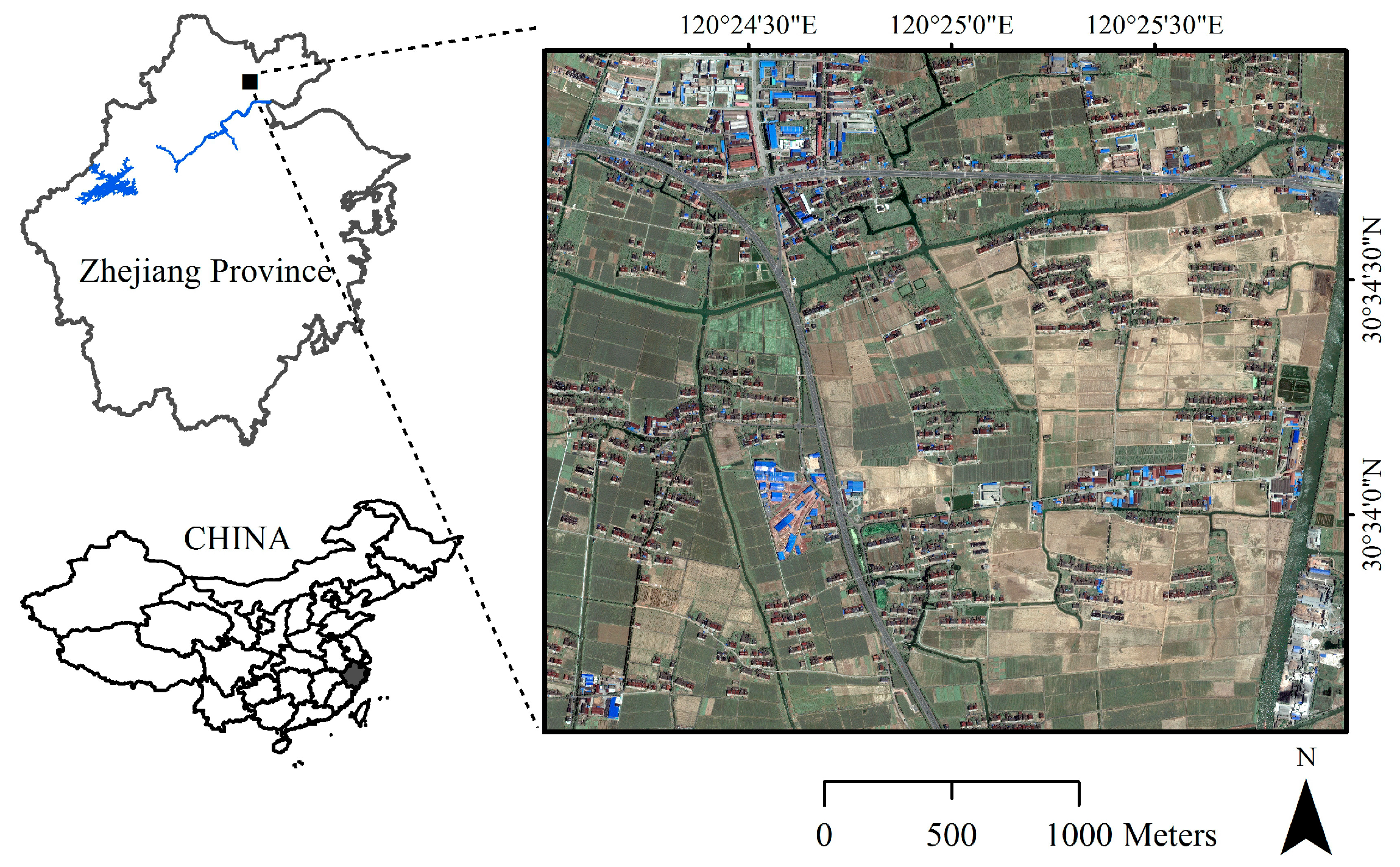
Detailed information regarding the land-use type, spatial area and distribution of buildings within rural regions is in urgent need for effective land resource management, energy supply management, environmental management and policy making. Residential and industrial building type remain ambiguous in current rural LULC maps. This circumstance impedes the process of precisely mapping rural areas for sustainable land-use development. Insufficient supervision on settlement and industry land leads to a tremendous waste of land resources and inefficient land exploitation within agricultural land.
Compared to urban land-cover types, rural land-cover categories have specific characteristics. Rural regions contain a larger number of vegetation cover or non-built cover than cities. In rural land, artificial surfaces such as rooftops, settlements, agricultural facilities, roads, etc., are sparse and have smaller occupied area.
Due to the fine spatial resolution, it becomes possible to identify the minimum feature such as a single rooftop in remotely sensed VHR imagery. Thus, VHR images could provide timely and tangible information for automatically subdividing rural settlement and industrial land-use types. Object-based image analysis (OBIA) fills the gap between pixels and real-world land cover objects [
9], which is similar to human perception [
10], and was proven to have produced a significantly higher accuracy than traditional pixel-based classification approaches employed in VHR images.
The processing units in OBIA method are not pixels but objects after segmentation, therefore a number of object features characterizing the spatial and textural information can be exploited to facilitate mapping accuracy [
9]. Previous studies have demonstrated that textural features [
11,
12], gray-level co-occurrence matrix (GLCM) [
13], local indicators of spatial association (LISA) [
14] information and local spatial statistics [
11] can be considered as features in OBIA classification procedures.
Furthermore, spatial and textural properties extracted from the image objects in object-based image analysis was proven to have made valuable contributions in discrimination or distinction heterogeneity among land-use categories that are difficult to distinguish, e.g., different land-use types with similar land-cover, or same land-use types with distinct spatial distribution pattern. For settlement or residential building discrimination purpose, Niebergall [
15] presented a hierarchical network embedding GLCM to distinguish between different settlement structures as well as land-cover classes. Owen’s research [
3] demonstrates that land-cover surface texture and geomorphic properties are significantly different between squatter settlements in suburban areas and well-established settlements in urban areas. Some researchers invented new index for distinguishing building types, particularly in rural areas. Kuffer [
16] used unplanned settlement index (USI), which integrated morphological features to distinguish between planned and unplanned areas from VHR data. Vegetation sample-based vegetation index, chessboard segmentation and average contrast of objects were used for extraction of plantation [
17].
This spectral and textural information mentioned above was derived from the object itself, and the contextual information about the relationship between the object and its surroundings or circumstances still has potential in classification application. Han [
14,
18] proposed a multi-scale approach incorporating textural and contextual information in hierarchical network of image objects to analyze of forest ecosystems of a complex nature.
Moreover, by using contextual information, some researchers used spatial statistics methods to improve discrimination techniques, such as local indicators of spatial association (LISA) measures, effective mesh size [
19] and lacunarity. Lacunarity was used to identify informal settlements from a high resolution binary imagery [
20]. Ma [
21] successfully discriminated residential and industrial buildings by integrating lacunarity algorithm, object-based segmentation and a decision tree classifier.
Different land-use behaviors will form different land-use units, which have different landscape pattern characteristics [
22]. In addition to spatial statistical methods for describing the landscape pattern, there are other means such as landscape metrics. Landscape metrics were designed to quantify the pattern of the landscape within the designated landscape spatial unit [
23]. In other words, landscape metrics contain the information of relationship between different land-use features. Therefore, landscape metrics have the potential to be integrated into the object-based classification. Facilitated by recent advances in computer processing and geographic information (GIS) technologies, a variety of landscape metrics have been developed for calculate landscape pattern [
24], including metrics describe area, edge, shape, aggregation and diversity in path level, class level and landscape level [
23]. Although these metrics were not designed for the classification phase of image processing, some studies have suggested and succeeded in using landscape metrics for image classification [
19,
25].
This paper applied landscape metrics to discriminate settlement and industry landscape units. After land-cover map is derived from VHR image, a chessboard segmentation was used to generate uniform landscape spatial units. Landscape metrics that characterize area proportion, shape, edge, aggregation and diversity properties were collected and adopted in classification algorithm. Three different classification schemes are compared: the method proposed, hierarchical classification using only spectral and textural properties, and hierarchical classification integrating lacunarity algorithm.
3. Methodology
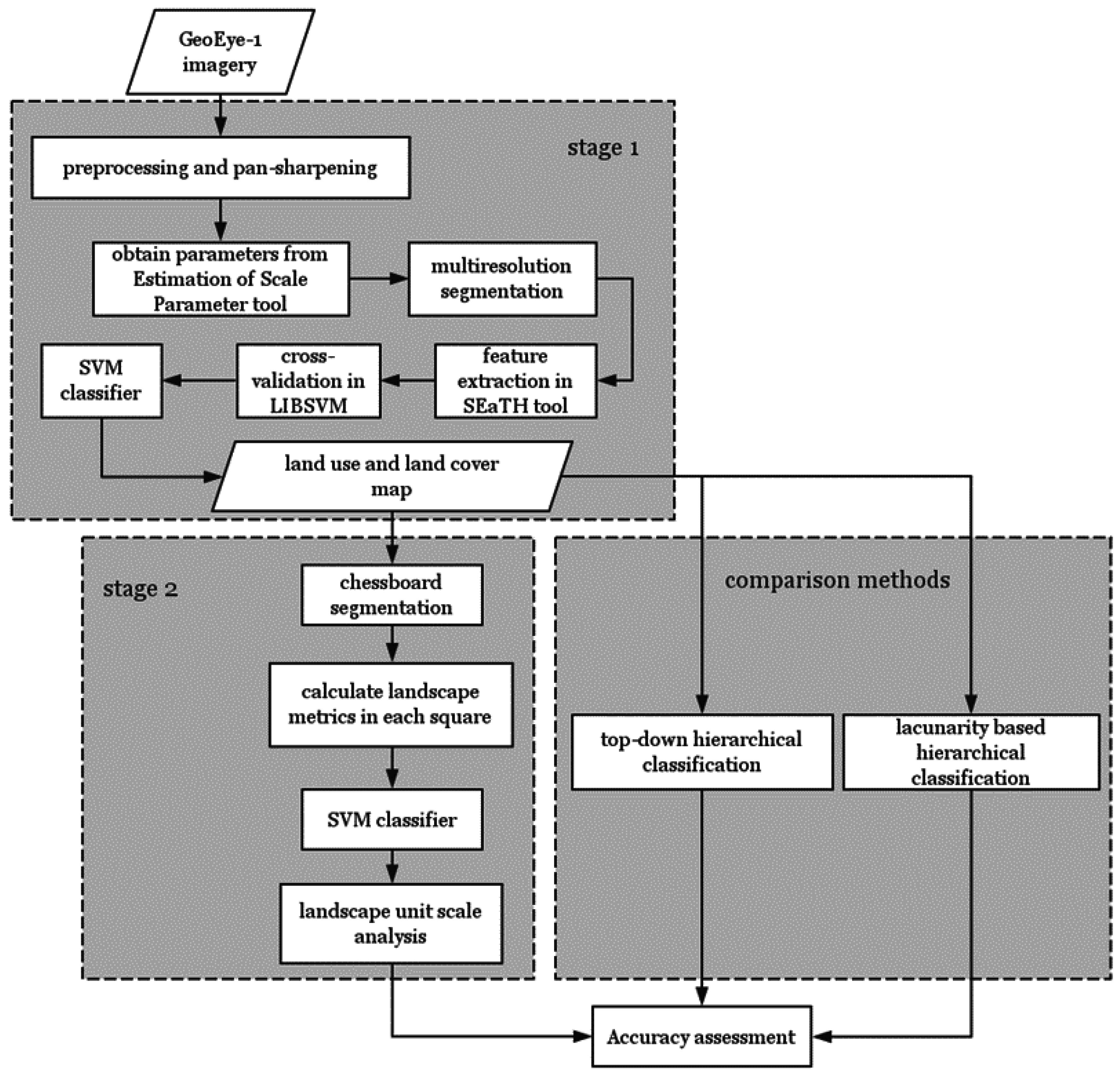
The classification approach we proposed is twofold. Land-cover information was derived in Stage 1, and settlements and industry area was distinguished in Stage 2. In order to verify whether the proposed method can effectively improve the classification accuracy, this study also used other two classification methods based on the result from Stage 1:
Top-down hierarchical classification network using only spectral, textural and shape properties; and
Hierarchical classification integrating lacunarity properties.
3.1. Stage 1: Mapping Land-Use and Land-Cover (LULC) Using OBIA
In order to ensure the simplicity of the entire distinction process, a single-scale non-hierarchical classification approach was adopted in eCognition
® (v9.0, Trimble Germany GmbH, Munich, Germany) in this stage. First, a segmentation algorithm was operated and a set of objects (segments) was generated, which was semantic meaningful. Many papers used multiresolution segmentation embedded in eCognition software package [
27,
28,
29]. Multiresolution segmentation is also known as Fractal Net Evolution Approach (FNEA), which is based on region growing methods and based on some certain homogeneity criteria: scale parameter, shape and compactness [
30,
31].
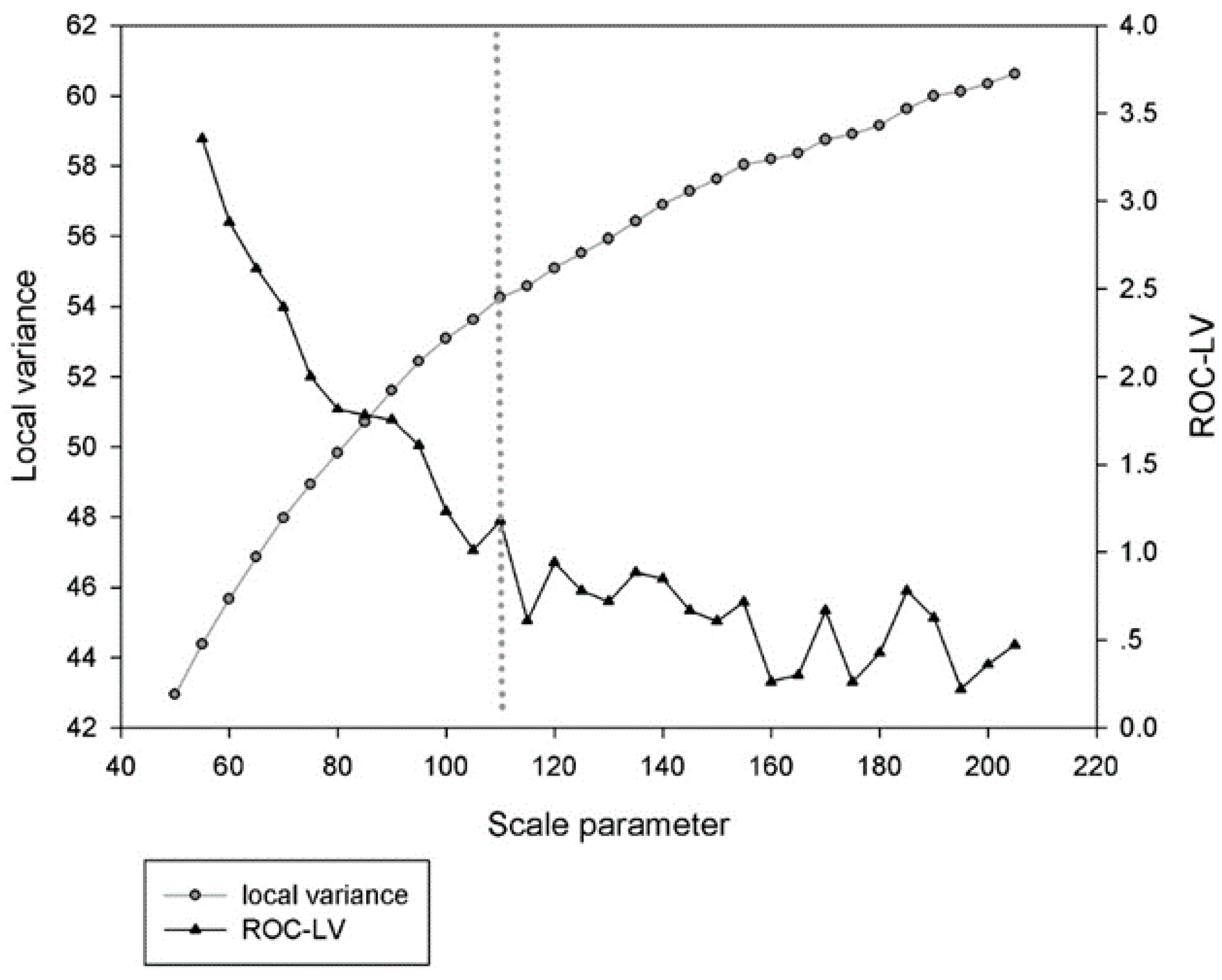
Usually, optimum segmentation parameters were obtained by subjective manual trial-and-error test. To make our framework operational and portable, an objective method named Estimation of Scale Parameter, i.e., ESP2 tool [
32], was used to identify the statistically most suitable scale parameter for segmentation algorithm. ESP tool iteratively generates image-objects at multiple scale levels in fixed step size and calculates the local variance (LV) in each scale. The rates of change of LV (ROC-LV) were plotted against the corresponding scale in
Figure 4. Based on the plot diagram, the peaks of the curve indicated appropriate scale parameter for segmentation [
33,
34,
35]. The scale of 110 appeared promising as the first break in ROC-LV curve after continuous and abrupt decay. Dotted vertical lines indicated optimal scale parameters in
Figure 4. As a result, we set segmentation scale as 110.
A visual assessment showed that the ESP2 tool identified the suitable scale parameter accurately to delineate meaningful objects, especially rooftops and concrete materials.
The shape and color parameters were weighted equally as 0.5, whereas the compactness was prioritized instead of smoothness and set as 0.8 because we focus on extracting buildings, especially the rooftops of settlements and industrial area which are more compact spatially.
After creating these objects, support vector machine (SVM) classifier was employed to identify the LULC types [
36,
37]. An automatic methodology called SEparability and THresholds (SEaTH) [
38] tool was adopted in feature selection step to seek significant features of optimal class separation [
15,
39]. SEaTH calculates the separability in Jeffries–Matusita distance and the corresponding thresholds of object classes for any number of given features on training examples. Eventually, mean values of brightness and all image bands, Normalized Difference Vegetation Index (NDVI), standard deviation, and GLCM (homogeneity, contrast, dissimilarity, entropy, angular second moment, mean, standard deviation and correlation) are selected as optimal feature subset and used in SVM classifier. All these features are normalized before classification applied. An SVM radial basis function (RBF) kernel was applied using the optimal parameters obtained from 5-fold cross-validation in LIBSVM [
40].
One thing to note here is that asphalt and water were not treated as automatic classification categories. Instead, we used land-use map from the National Detailed Land-Use Inventory to assign these types directly. For asphalt category, this material is not universal, and there are only two lanes throughout the study area. Thus, it represents only 1% of the total number of objects after segmentation. Meanwhile, water cover surface is often covered by tree canopy, or aquatic plant, resulting in classification confusion with other land-cover types. Similar to asphalt, water surface only contains the linear feature of canal and few ponds in the study site. It is not only time-consuming, but could also cause harmful effect on other terrain categories’ accuracy, for example classify them as asphalt and water cover.
3.2. Stage 2: Landscape Metrics and Chessboard Segmentation
After the Stage 1, the LULC map is derived from Geoeye imagery. However, the area of residential and industrial cover is still unrevealed. In Stage 2, contextual information from inside different land-use units was applied to discriminate settlement and industrial area.
The composition, structure and pattern characteristic of different land-cover objects within a land-use unit, compose valuable information reflecting land use behavior. This information can be described and quantified by landscape metrics.
Defining land-use units is crucial for further landscape patterns analysis. Therefore, a chessboard segmentation was applied to the LULC map derived in Stage 1 to create land-use units, i.e., chessboard square, for further calculating landscape metrics. Chessboard segmentation is a simple segmentation algorithm. It cuts the image into equal square objects of a given size. Block squares (or fishnet squares, or chessboard squares) are commonly used to describe the landscape characteristics of the urban growth [
41] and agricultural landscape patterns [
42]. Chessboard segmentation can keep the spatial units in a uniform size. In this form, landscape features become comparable among spatial units, i.e., separable or categorizable. It is obvious that chessboard segmentation is a scale-dependent approach. In this paper, we tested different chessboard scales ranging from 40 m to 100 m, with 20 m step-size.
Landscape metrics that characterize area, shape, edge, aggregation and diversity properties were collected as feature space for classification. Percentage of Landscape (PLAND) of each LULC types, Number of Patches (NP), Total Edge (TE), Landscape Shape Index (LSI) and Shannon’s Diversity Index (SHDI) were calculated for each unit and used as features in SVM classifier (
Table 1). The RBF kernel was applied again and still using the optimal parameters. Those chessboard squares were classified into three categories: settlement unit, industry unit and other unit. Twenty classification examples for each category are manually selected. Eventually, artificial land-cover types that intersect in settlement unit or industry unit were reclassified into settlement or industry area respectively.
3.3. Top-Down Hierarchical Classification
In order to compare the accuracy of classification, this study also used two other methods to distinguish between these two built-up types. Based on the land-cover map derived from Stage 1, a top-down approach was applied under the results of the first level of classification. Concrete, clay rooftops and metal rooftops were separated into settlement and industry subclasses. Three artificial land-cover types were subdivided into six categories, e.g., settlement clay rooftops and industry clay rooftops. It is noteworthy that there was no new segmentation process in this classification stage, using only the segments generated from Stage 1. Twenty classification examples were equally selected and then the SVM was used to further distinguish settlements and industrial area. More features were added into the classifier. Rooftops and harden ground material in settlements are smaller in objects’ geometry, and also are different in shape. Therefore, geometry metrics containing area, length, width, length/width, asymmetry, border index, compactness, density, roundness, shape index of extend and shape attributes were add into features for classification.
3.4. Lacunarity Based Hierarchical Classification
In addition to the landscape metrics, there are spatial statistics methods to analyze landscape spatial pattern, e.g., the lacunarity. Lacunarity is a measure of “gappiness” or “hole-iness” of a geometric structure and has been used to describe the distribution of the gap sizes in a fractal sequence [
43]. Lacunarity algorithm was demonstrated in discriminating land-use types or building types in some urban area [
20,
21]. In this paper, a lacunarity properties based hierarchical classification was compared with the other two methods. Lacunarity analysis can be based both on binary and grayscale images [
44]. Here, we generated build-up areas/non-build-up areas binary images on Stage 1 classification result, and assigned values of 1 or 0, respectively. Lacunarity analysis is carried out in an extension implemented in ArcGIS software [
45]. The lacunarity Λ(r) at scale r can be defined as:
where S represents occupied sites, and
represents the probability of distribution of occupied sites S, which can be obtained by dividing
by the total number of boxes.
Lacunarity is a function of window size and gliding box, so it is important to identify the optimal size by lacunarity-window size plot. This value can be determined when the image appears as self-autocorrelation. Under these circumstances, three consecutive points on the lacunarity curve are linear, and the coefficient of determination (
r2) approaches 1 [
43].
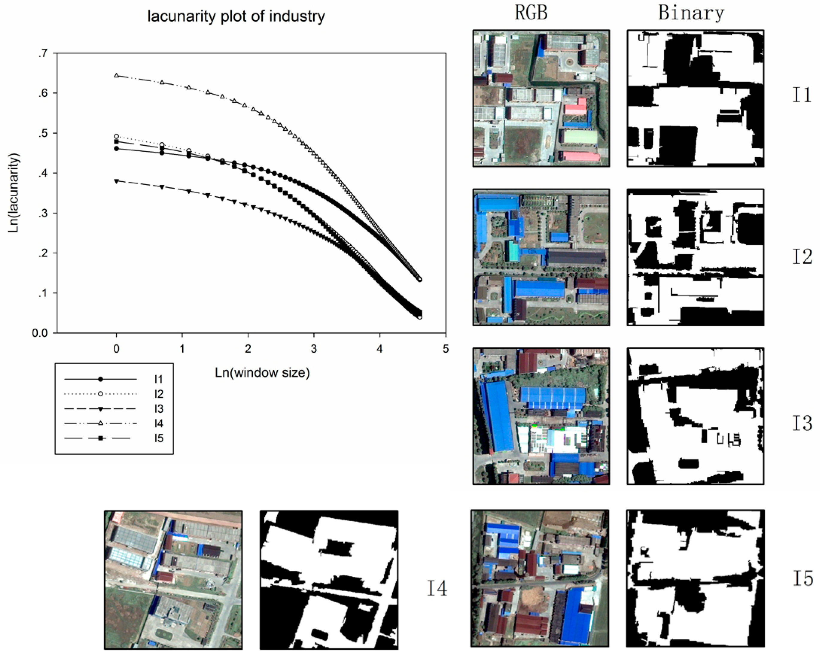
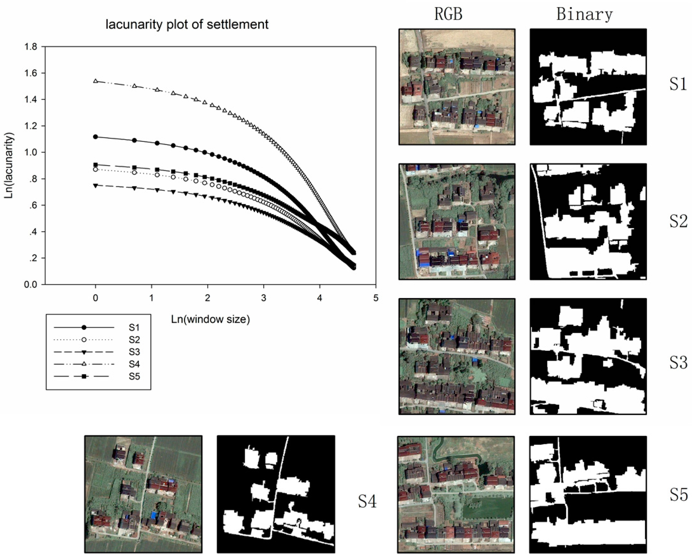
The relationship between window-size and lacunarity was analyzed based on 200 m× 200 m examples.
Figure 5 illustrated how the lacunarity plots vary with increasing window scale in both settlement and industry area.
Rural settlement area appears as smaller and more scattered patchy built-up areas with larger percent of gaps in analyzed examples than industrial area; meanwhile, gaps in rural settlement area seem more irregular in distribution. Consequently, settlement areas present higher lacunarity than industry areas. As window size increases, the lacunarity values decreased dramatically. For comparison, two types of land-use lacunarity normalized curves were analyzed. In general, land-use features appeared to self-autocorrelate at around 35 window size, implying the quasi-linear decrease in the normalized lacunarity plot. As a result, optimal window size was set as 35. With gliding-box sizes of 3 × 3, 5 × 5, 7 × 7, and 9 × 9, four lacunarity features were calculated for subsequent classification.
3.5. Accuracy Assessment
Accuracy statistics, including producer’s accuracy (PA), user’s accuracy (UA), overall accuracy (OA), and kappa coefficient were calculated based on the error matrix [
46]. An error matrix that expresses the number of sample segments assigned to a particular LULC category relative to the actual category is created. The producer’s accuracy is a measure of omission error, indicating the probability of an actual category being correctly classified, whereas the user’s accuracy is a measure of commission error, indicating the probability that a segment classified on the image actually represents that actual category. Overall accuracy is the percentage of correctly classified samples. Kappa analysis is a widely-used and powerful multivariate technique for accuracy assessment. The estimate of kappa is the so-called Kappa coefficient. Kappa coefficient is a measure of overall statistical agreement of a confusion matrix. Therefore, it provides a more rigorous assessment of classification accuracy [
47].
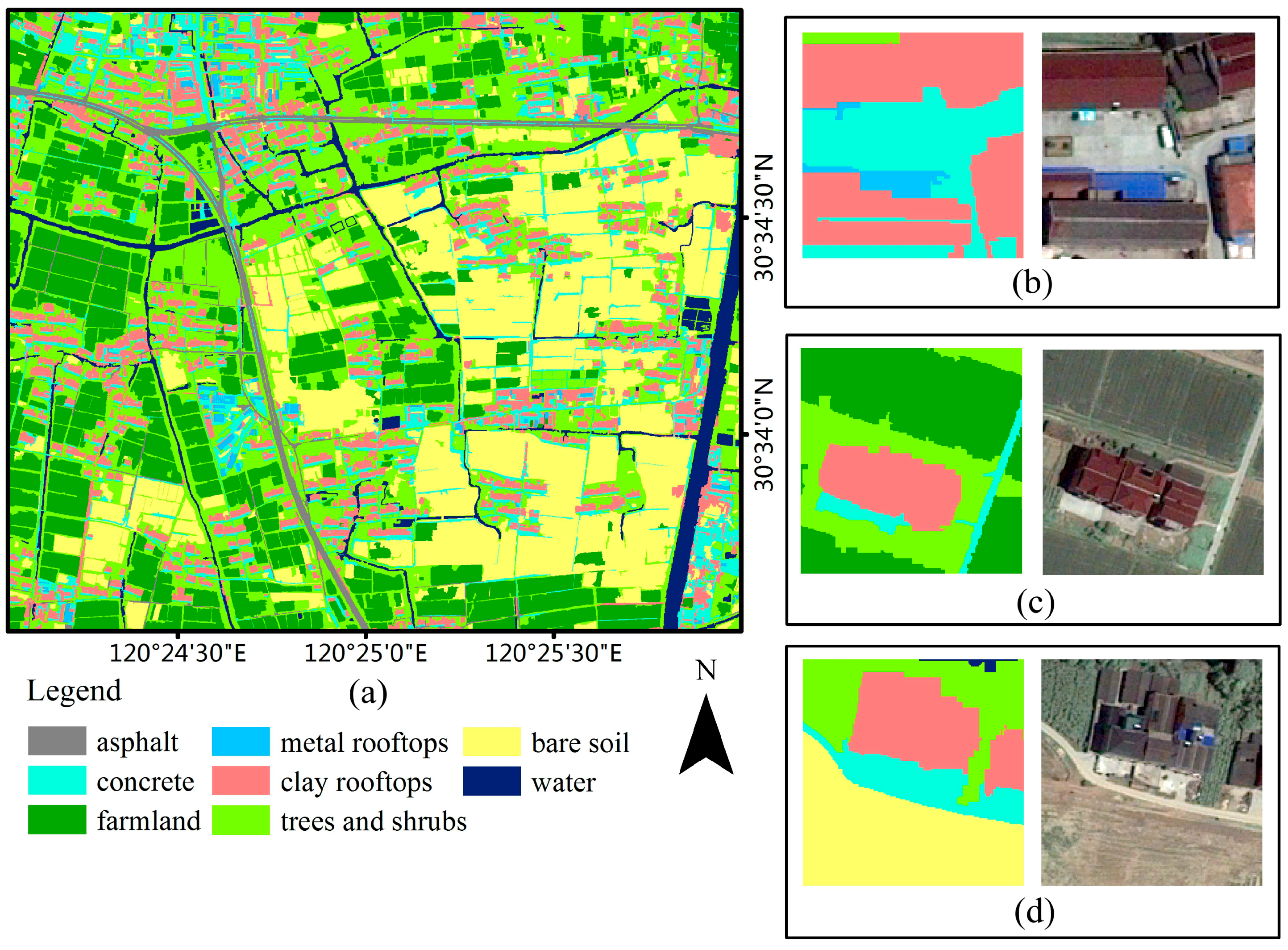
In Stage 1, a real land-use and land-cover map was generated through visual interpretation. In visual interpretation step, we used National Detailed Land-Use Inventory Maps in 2011 as reference data (
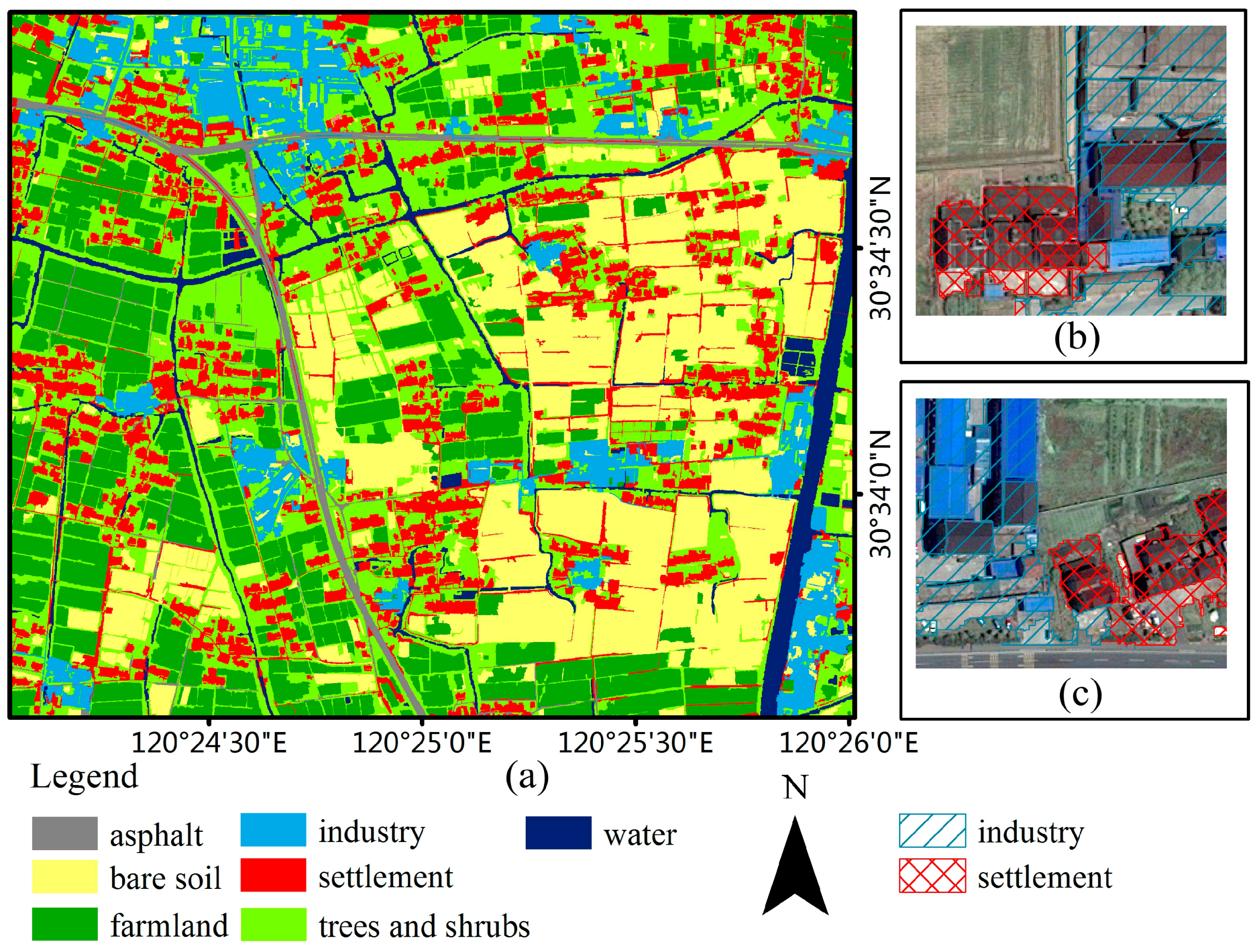
Figure S1). Then, the error matrix was calculated after randomly selected segments were compared with the real land-use and land-cover vector data. In Stage 2, a ground investigation was conducted to confirm that the selected segments are industrial or residential area.
In total, 956 randomly selected segments were used for construction of the error matrix for Stage 1. Among these segments, the man-made objects, i.e., concrete and rooftops, which were classified correctly, were collected to generate error matrix to enable the scale analysis in Stage 2 and the comparison between three different classification approaches. Totally, 467 artificial class objects were collected and no less than 220 objects for settlement and industry types each. A fully rigorous and exhaustive approach named McNemar test was adopted for expressing the statistical significance on different classification results [
48]. Z values were calculated on every paired result combinations. A z value matrix clearly identified those classification pairs that are significantly different and those that are not. With four scales of chessboard and two other hierarchy classification approaches, there are a total of 15 z values in the matrix.
6. Conclusions
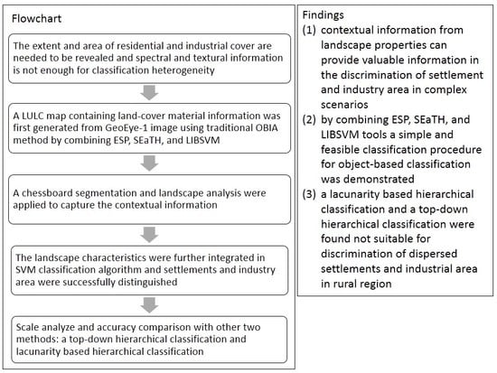
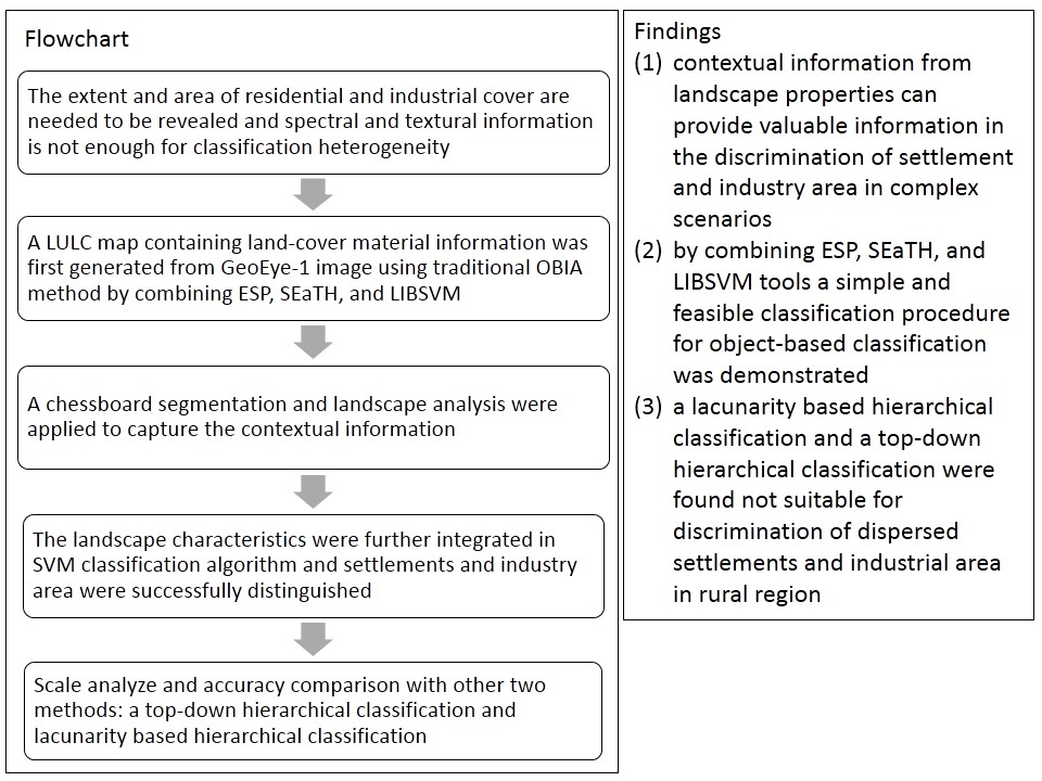
In order to obtain precise information of land-use and discriminate settlements and industrial area in rural areas, this paper demonstrates a classification scheme integrating OBIA, landscape metrics and chessboard segmentation. A LULC map containing land-cover material information was first generated from GeoEye-1 image using traditional OBIA method. Next, a chessboard segmentation and landscape analysis were conducted to capture the contextual information between the object and its surroundings in each unit. The landscape characteristics were further integrated in SVM classification algorithm, and settlements and industry area were successfully distinguished.
Two commonly used approaches, i.e., the top-down hierarchical classification network using spectral, textural and shape properties, and lacunarity based hierarchical classification were also tested in our study. The comparative analysis demonstrates that our method performed better and produced more accurate results than the two other approaches, with the highest overall accuracy, Kappa coefficient and McNemar test. Thus, the landscape properties can contribute to the discrimination of settlement and industry area in complex scenarios.
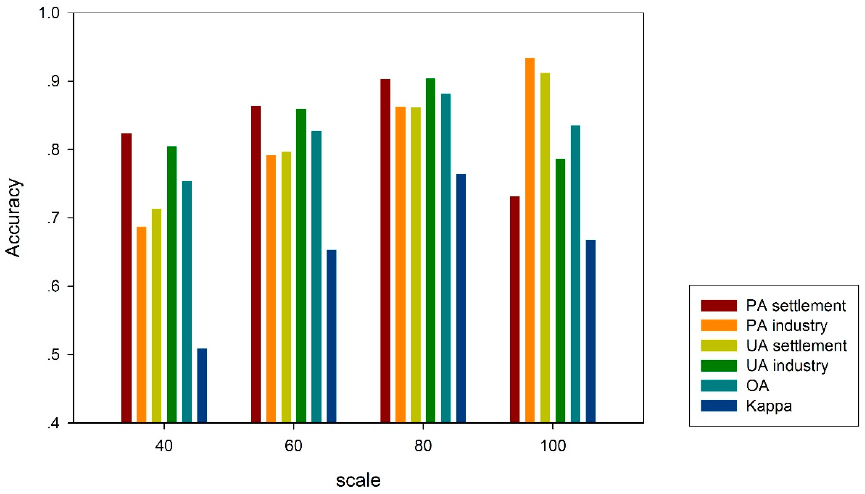
Furthermore, the scale dependence of our method was also tested by analyzing the classification accuracy at various scales, i.e., 40 m, 60 m, 80 m, and 100 m. The overall accuracy ranged from 75% to 88%, and Kappa coefficient ranged from 0.51 to 0.76, both peaking at scale 80 m. The optimal scale parameter was found to be related to the size of the building blocks in industry area.


 ,
, 


