In this section, three sets of real hyperspectral datasets, collected by different imaging sensors, are used to perform experimental evaluation for the proposed algorithm.
4.1. Optimum Kernel Parameter on the LRTC-KRXD
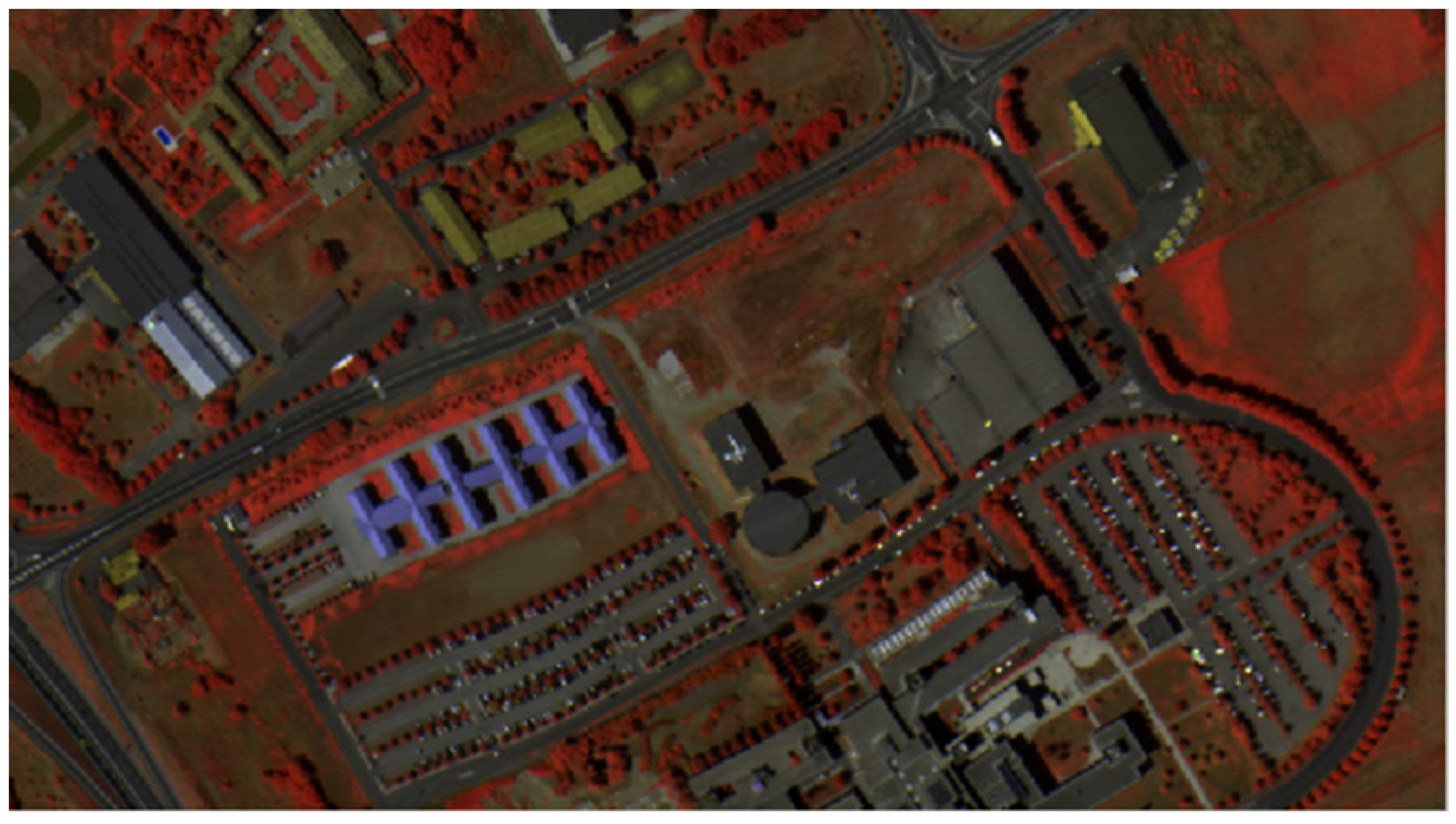
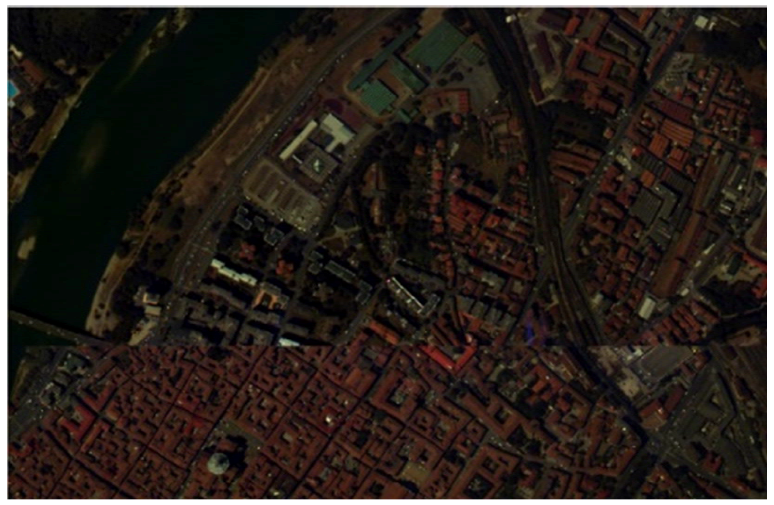
This group of experiments explores the optimum Gaussian radial basis function kernel parameter on the LRTC-KRXD. In the experiments, by virtue of cross-validation, the local causal sliding window width in the LRTC-KRXD on the PaviaU dataset, Pavia Center dataset, and San Diego Airport dataset is manually set to be 70, 40, and 70, respectively.
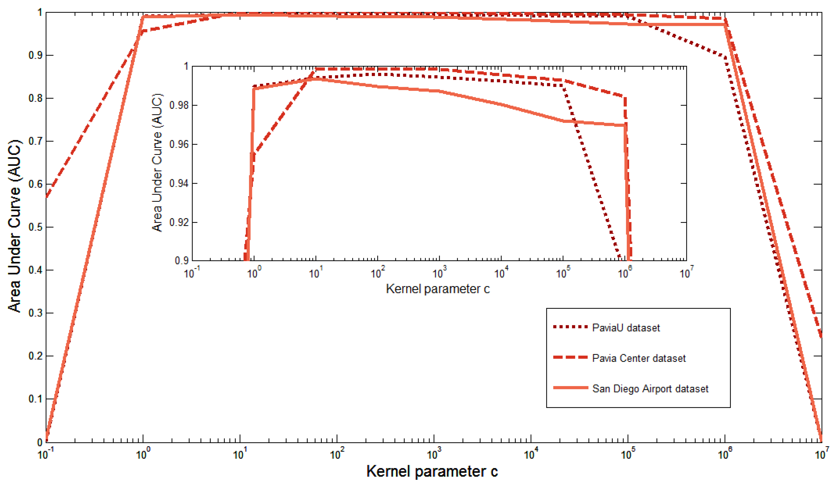
The receiver operating characteristics (ROC) curve representing detection probability versus false-alarm rates is a strong technique to present quantitative performance analysis. Area under the ROC curve (AUC) is also used to judge the performance of hyperspectral detection.
Figure 8 gives the different AUC of the LRTC-KRXD with changing kernel parameter
for all three hyperspectral images. For the PaviaU dataset, the AUC is the largest when
is equal to 100. For the Pavia Center and San Diego Airport datasets, however, the LRTC-KRXD shows the best AUC when
is up to 10. From
Figure 8, the AUC for all three datasets rises rapidly between
and
, then they keep basically smooth until
, which is followed by a steady drop before
. Therefore, the kernel parameter
is not sensitive to the LRTC-KRXD in some very long numerical range.
4.2. Effects of the Local Causal Sliding Array Window Width on the LRTC-KRXD
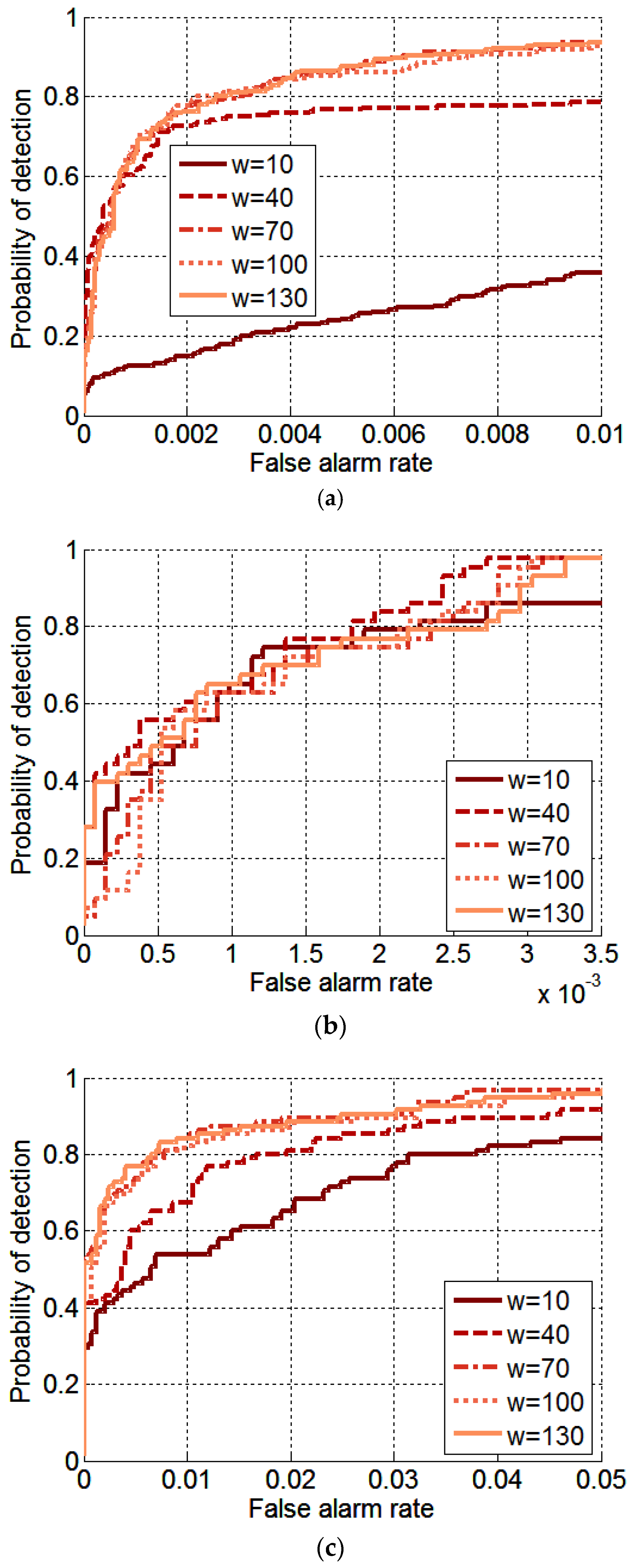
This group of experiments investigates the performance sensitivity of the LRTC-KRXD in terms of local causal sliding array window width. In these experiments, the local causal sliding array window width in the LRTC-KRXD on three images is manually set from 10 to 130 with steps of 30. By using cross-validation, the parameter of the Gaussian radial basis function kernel in LRTC-KRXD is set at 100 on the PaviaU dataset and 10 on both the Pavia Center and San Diego Airport datasets.
Figure 9 shows the ROC curves of the LRTC-KRXD on three images using changing local causal sliding array window width
w between 10 and 130. For the PaviaU dataset in
Figure 9a, the detection effect is poor using the local causal sliding array window width
w = 10, but the detection performance starts to improve as the local causal sliding window width grows. When it is greater or equal to
w = 70, the local causal sliding array window detection performances are comparable. For the Pavia Center dataset in
Figure 9b, the ROC curve result with the local causal sliding array window width
w = 10 performs the worst, however, the detection accuracy increases when the local causal sliding window width rises. When
w = 40, their ROC curves are similar. For the San Diego Airport dataset in
Figure 9c, the detection performance improves as the local causal sliding window width
w rises from 10 to 70. When it continues to grow, the ROC curve result remains basically unchanged.
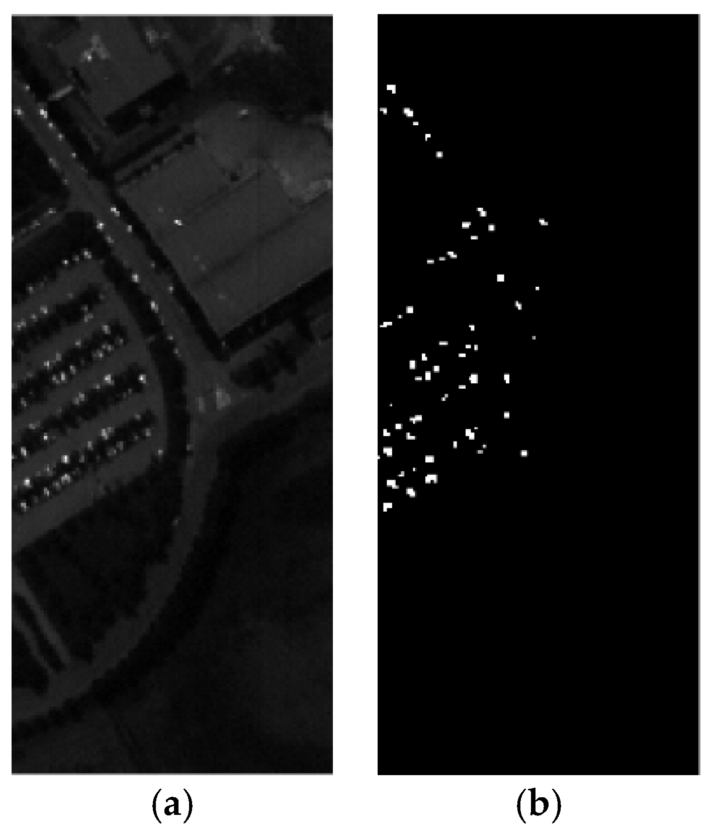
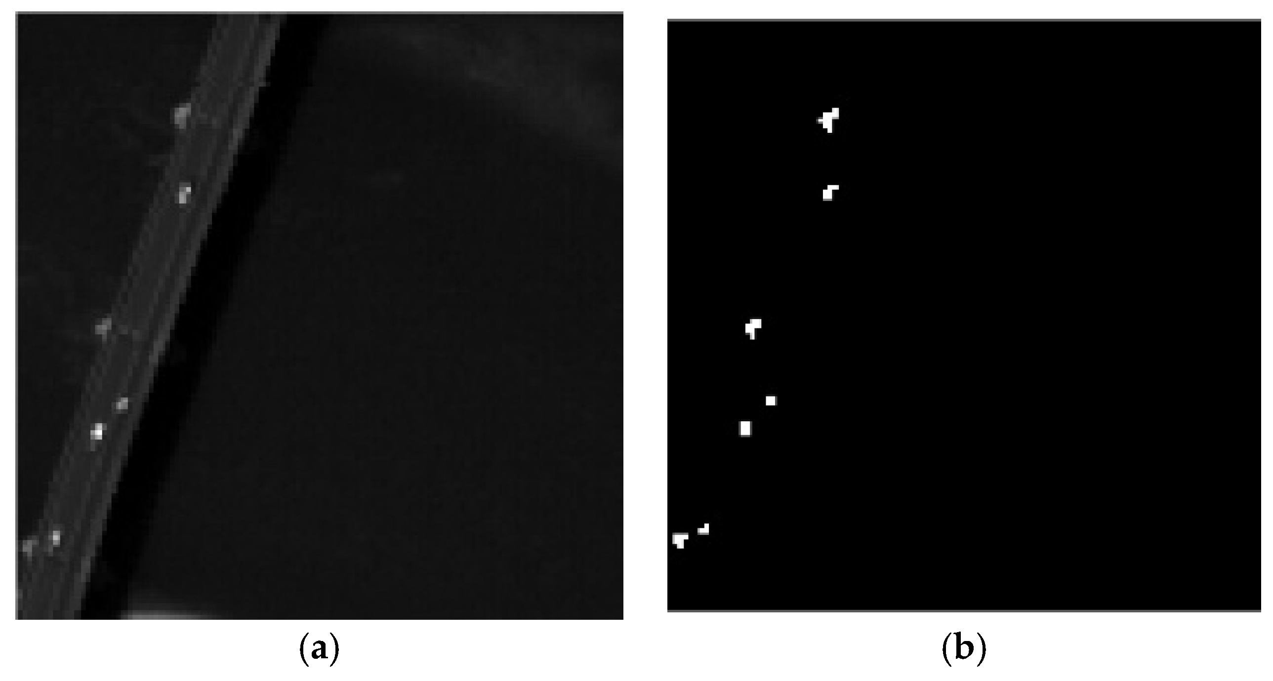
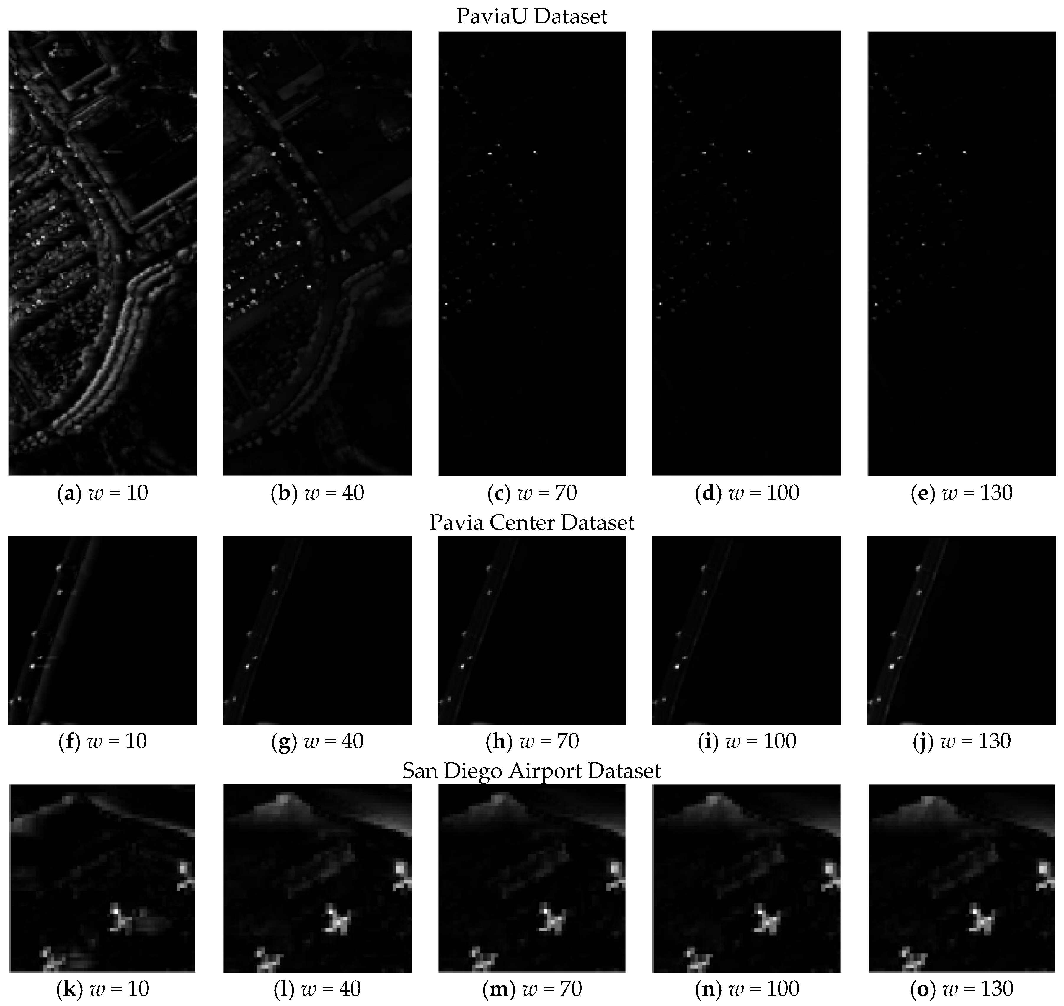
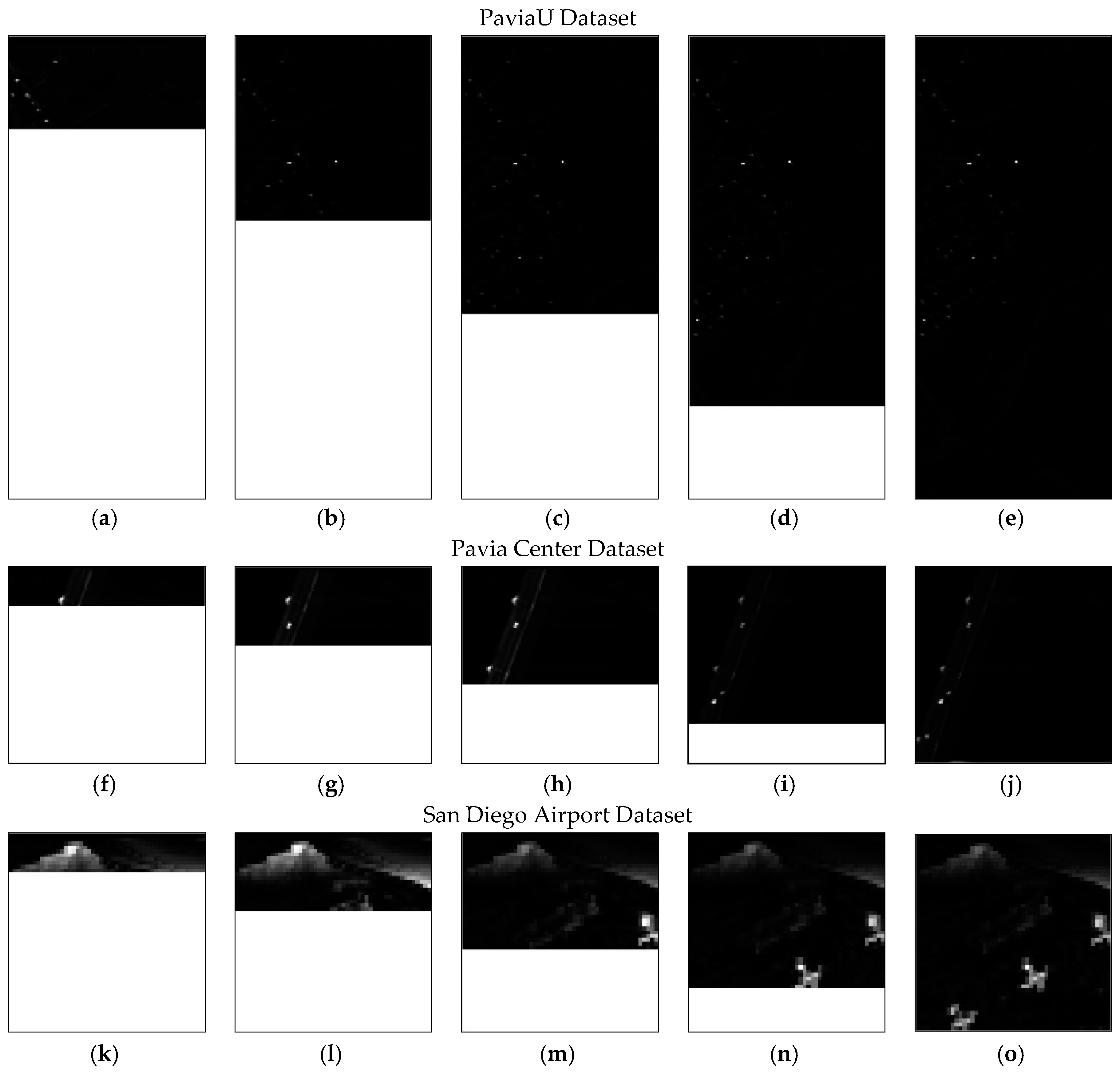
Figure 10 reveals the grayscale results of the above experiments. When the local causal sliding window width
w = 10, shown in
Figure 10a, f, and k, there is a bad detection effect on the pixels next to the large anomaly in the direction of the window. This is because at those positions, with the small local causal sliding array window width, backgrounds are easily corrupted by the anomalies involved in the local causal sliding array window. As the local causal sliding array window width increases, such phenomena disappear gradually since the number of background pixels in the local causal sliding array window grows. When the local causal sliding array window widths of the LRTC-KRXD on the PaviaU, Pavia Center, and San Diego Airport images are greater or equal to
w = 70,
w = 40, or
w = 70, respectively, their own grayscale outputs are similar by visual inspection.
4.3. Detection Performance of the LRTC-KRXD
These experiments explore the detection performance of the LRTC-KRXD. We made comparisons between the LRTC-KRXD and three other anomaly detectors on three hyperspectral datasets. The other three anomaly detectors included two real-time detectors (GRTC-RXD and LRTC-RXD) and one non-real-time detector (LKRXD). In these experiments, for the LRTC-KRXD, by cross-validation, the parameter of Gaussian radial basis function kernel is set to 100 on the PaviaU dataset and to 10 on both the Pavia Center dataset and the San Diego Airport dataset. The local causal sliding array window width, w, on the PaviaU dataset and San Diego Airport dataset is set to 70, and the local causal sliding array window width, w, on the Pavia Center dataset is set to 40. For the LRTC-RXD, the local causal sliding array window width, w, on the PaviaU, Pavia Center, and San Diego Airport datasets is set to 400, 300, and 300, respectively, to obtain the best, stable outputs. For the LKRXD, by cross-validation, the set of the kernel parameter is the same as the LRTC-KRXD on all three images, but the size of the inner window and outer window in the LKRXD is set to 5 and 11, respectively.
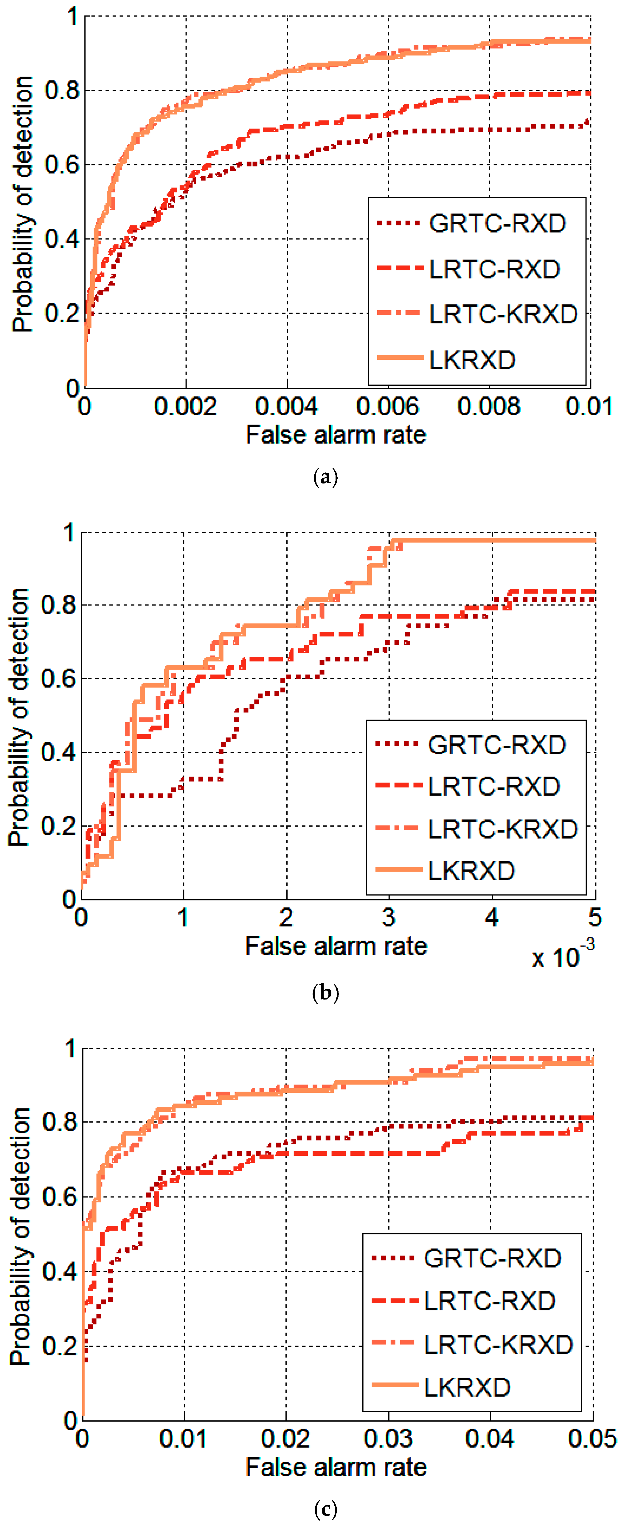
Figure 11 shows the results of the ROC curves from all three real-time anomaly detectors and one non-real-time anomaly detector on the three HSI datasets. For the PaviaU dataset shown in
Figure 11a, the LRTC-KRXD and the LKRXD are similar throughout the curves, and compared to the GRTC-RXD and the LRTC-RXD, they show a much higher detection probability. For the Pavia Center dataset shown in
Figure 11b, the ROC curve results of the LRTC-KRXD and the LKRXD are comparable, but they far outperform those of the GRTC-RXD and the LRTC-RXD. For the San Diego Airport dataset, similar detection effects related to the LRTC-KRXD and the LKRXD are shown in
Figure 11c, and these detection effects are better than those of the GRTC-RXD and the LRTC-RXD. This result is because the recursion process of the LRTC-KRXD is derived from the LKRXD that mines nonlinear information by a kernel trick, and there is no information leaked out in this process. Some small differences occur between the detection results of the LRTC-KRXD and the LKRXD because the pseudoinverse of the Gram matrix generally needs to be implemented when each pixel is detected in the LKRXD [
32], while this is avoided by recursion in the LRTC-KRXD; the local dual window is used in the LKRXD while the local causal sliding array window is used for the LRTC-KRXD.
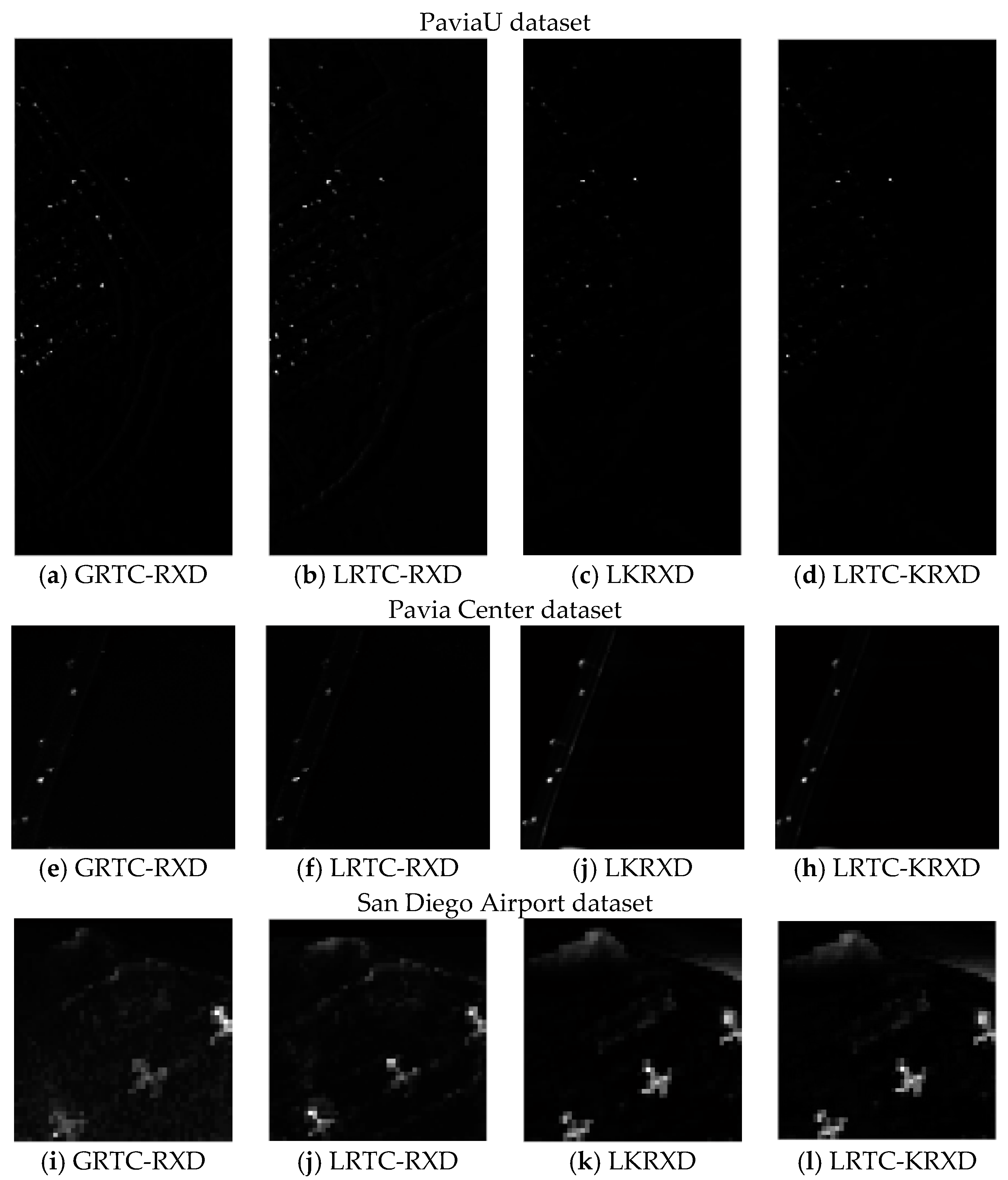
Figure 12 presents the grayscale outputs of ther GRTC-RXD, LRTC-RXD, LKRXD and LRTC-KRXD on three hyperspectral images. For the PaviaU dataset and the Pavia Center dataset, by visual inspection of
Figure 12c,d,g,h, there are no appreciable differences, but they clearly show better grayscale results compared with that of
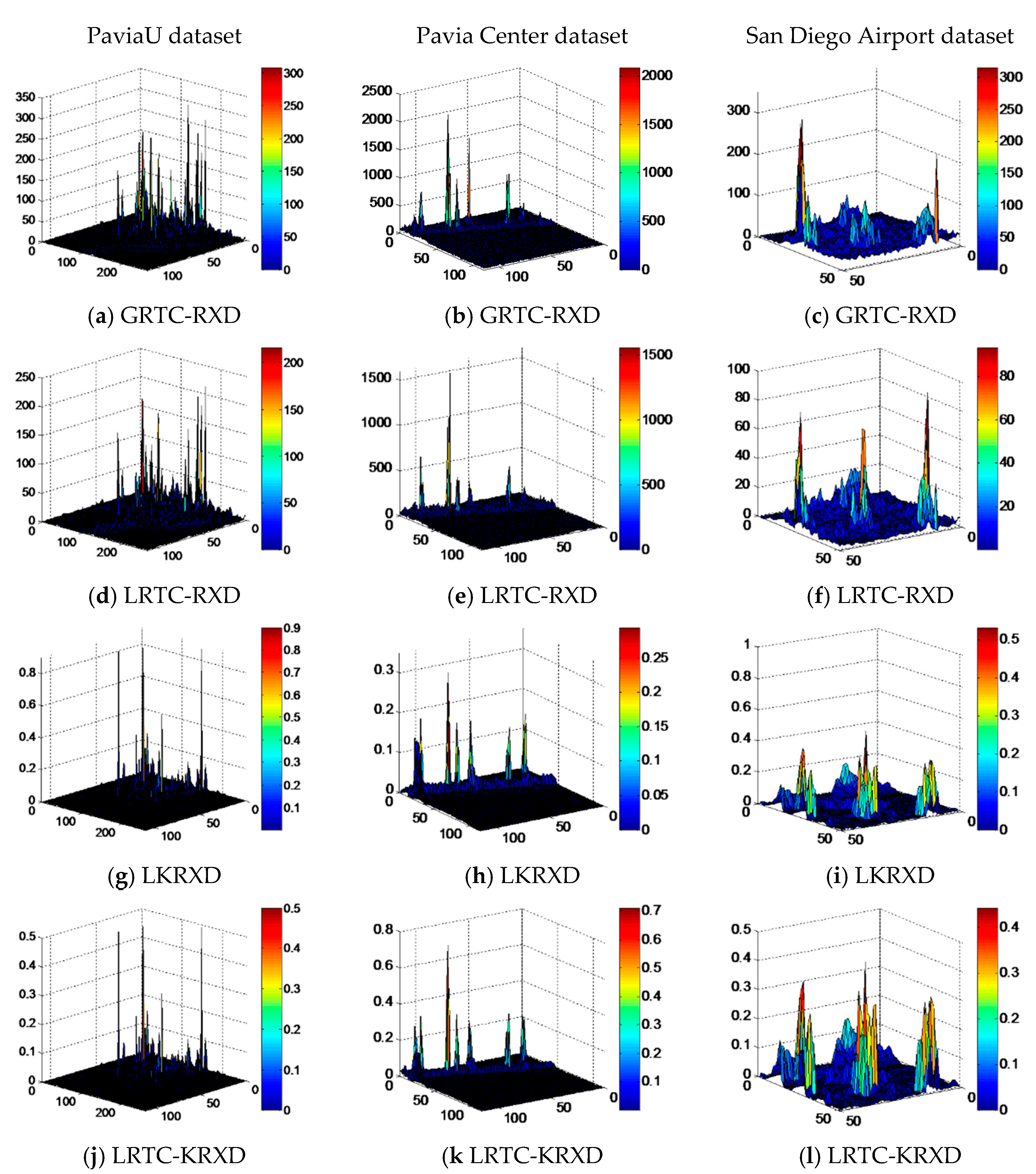
Figure 12a,b,e,f. For the San Diego Airport dataset, better background suppression is shown in the LRTC-KRXD and the LKRXD. Three-dimensional (3D) plots are used to verify the detailed differences among the GRTC-RXD, LRTC-RXD, LKRXD, and LRTC-KRXD on the three hyperspectral datasets. As we can see from the 3D plots shown in
Figure 13, the detection results of the LKRXD and the LRTC-KRXD are comparable with better detection performances than those of the GRTC-RXD and the LRTC-RXD on both the PaviaU dataset and Pavia Center dataset. It is also clear in
Figure 13c,f,i,l that the 3D plots of the LRTC-KRXD and the LKRXD show the robust target clusters.
Figure 14 shows the progressive detection procedures of the LRTC-KRXD on the PaviaU, Pavia Center, and San Diego Airport datasets. By using the local causal sliding array window, anomalies in the hyperspectral images are detected pixel-by-pixel in real time. In addition, as time moves along, some weak anomalies appear with various levels of background suppression. For example, on the Pavia Center image, the first three weak anomalies display clearly in the progressive detection results, but when the strong anomaly is detected later, these weak anomalies become dim.
4.4. Computational Analysis of the LRTC-KRXD
Both computational complexity and computing time are significant indicators to measure the performance of anomaly detection, especially real-time processing. The computational complexity of the LKRX algorithm originates in the components of the LKRX formula specified by Equation (7), including the current pixel in the feature space
, the background data sample mean
, the Gram matrix
and its inversion
. First,
is of order
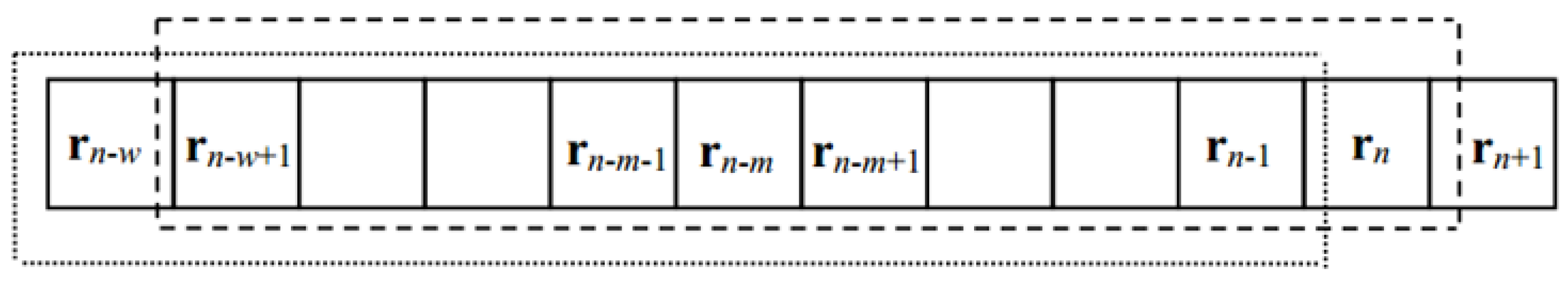
where ω is the size of the local causal sliding array window and
is the number of bands. It is not really possible to improve it since
in the equation of
is not constant when the local sliding array window moves. Second, for
, the multiplicative order is approximately
without recursive update processing, while using the recursive update equation given by Equation (23), the multiplicative order is close to zero. Third, the multiplicative order of
in the LKRXD is
, while in the the LRTC-KRX detector, due to the usage of recursive processing, the multiplicative order is not defined (“
” entries in
Table 4). Lastly, the multiplicative order of
is reduced to
from
by virtue of the matrix inversion lemma and Woodbury matrix identity. The more detailed computational complexity is shown in
Table 4, where we can see that
and
in the multiplicative order are not involved in LRTC-KRX detection, which reduces much of the computational complexity and cuts down on the massive computing time.
The computer environments used for the experiments were 64-bit operating systems with Intel(R) Core (TM) i7-4770K, 3.5 GHz CPU, and 16 GB memory (RAM). All the experiments were conducted five times and averaged to remove computer error [
15,
16].
Table 5 shows the total computing time of the LKRXD and the LRTC-KRXD on three hyperspectral datasets. By using recursive update equations, the total computing time of the LRTC-KRXD is reduced by at least 44-fold compared to the LKRXD.


