Haze Removal Based on a Fully Automated and Improved Haze Optimized Transformation for Landsat Imagery over Land

Abstract

Optical satellite imagery is often contaminated by the persistent presence of clouds and atmospheric haze. Without an effective method for removing this contamination, most optical remote sensing applications are less reliable. In this research, a methodology has been developed to fully automate and improve the Haze Optimized Transformation (HOT)-based haze removal. The method is referred to as AutoHOT and characterized with three notable features: a fully automated HOT process, a novel HOT image post-processing tool and a class-based HOT radiometric adjustment method. The performances of AutoHOT in haze detection and compensation were evaluated through three experiments with one Landsat-5 TM, one Landsat-7 ETM+ and eight Landsat-8 OLI scenes that encompass diverse landscapes and atmospheric haze conditions. The first experiment confirms that AutoHOT is robust and effective for haze detection. The average overall, user’s and producer’s accuracies of AutoHOT in haze detection can reach 96.4%, 97.6% and 97.5%, respectively. The second and third experiments demonstrate that AutoHOT can not only accurately characterize the haze intensities but also improve dehazed results, especially for brighter targets, compared to traditional HOT radiometric adjustment.

1. Introduction

Cloud and haze are two common atmospheric phenomena that often contaminate optical remote sensing images. The existence of these contaminations degrades image quality and can significantly affect remote sensing applications, such as land cover classification [1], change detection [2] and quantitative analysis [3]. For this reason, cloud and haze removal have become two essential pre-processing steps. Cloud and haze have different optical properties, and thus must be treated differently. Cloud normally blocks nearly all reflected radiation along the viewing path; hence, substitution with clear-sky pixels recorded at different time is usually suggested for recovering the lost surface information [4]. Haze generally refers to spatially varying, semi-transparent thin cloud and aerosol layers in the atmosphere [5,6]. The semi-transparent property of haze is twofold. On the one hand, it increases the difficulty of discriminating hazy pixels from clear-sky pixels, since the remotely measured signal of a hazy pixel is the mixture of the spectral responses from both haze and the land surface [7]. On the other hand, it leaves an opportunity for restoring true image information underneath hazy areas [8]. Except for desert haze, most haze types have much smaller impacts to near infrared (NIR) and shortwave infrared (SWIR) bands than to visible bands. For this reason, the emphasis of this study is on detecting and removing haze from visible bands. For high-altitude thin cirrus clouds, since they are very hard to detect with visible bands, a specific channel (e.g., the band around 1.38 μm implemented on MODIS, Landsat-8 and Sentinel-2) and method are needed [7,9,10]. An effective haze removal algorithm can be beneficial for many remote sensing applications, because more real surface reflectance can be exposed. This is particularly true when the satellite images to be used cannot be collected frequently (e.g., the revisit time of Landsat series satellites is 16 days). For large area or temporal applications demanding massive optical images, a fully automated haze removal method is highly desired [11].

A haze removal procedure generally consists of two consecutive stages: haze detection and haze correction. Haze detection is the process of obtaining a spatially detailed haze intensity map for an image, while haze correction is the algorithm for removing haze effects from an image based on the haze intensity map. It has been commonly recognized that the performance of a haze removal method is largely dependent on the accuracy of haze detection [6,8,12,13]. Since the distributions of atmospheric haze vary dramatically in both spatial and temporal dimensions, it is extremely difficult in practical applications to collect spatially detailed in-situ measurements of atmospheric haze conditions during the time of an image acquisition [14]. As such, a common practice to obtain a haze intensity map is estimation based on the contaminated image itself. Over the past decades, a large number of scene-based haze removal approaches have been proposed in the literature [6,8,12,13,14,15,16,17,18,19,20,21,22,23]. These existing methods fall into three general categories: dark object subtraction (DOS) [8,12,13,15,16,17], frequency filtering [18,19] and transformation based-approaches [6,14,20,21,22,23].

DOS-based methods were developed according to the physical principle of atmospheric effects on the image signals of dark targets. The radiative effects of atmospheric haze include scattering and absorption of sunlight in the sun–surface–sensor path. For dark surfaces, scattering effects (often known as path radiance) is a dominant and mainly additive component upon the total radiance measured by an optical sensor [12,15]. This indicates that it is appropriate to employ dark pixels in a scene to estimate path radiance, which is proportional to the haze optical thickness. Basically, the path radiance of a dark pixel can be estimated by subtracting a small predicted radiance from its measured at-sensor radiance. DOS-based methods have a long history and have evolved from the stage of only being suitable for homogeneous haze conditions [13] to the stage of being able to compensate spatially varying haze contaminations [8,12,15,16]. To make use of more dark objects present in a scene, Kaufman et al. [15] proposed a dense dark vegetation (DDV) technique, which is based on the empirical correlation between the reflectance of visible bands (usually blue and/or red bands) and that of a haze-transparent band (e.g., band 7 in the case of Landsat data) for DDV pixels. A DDV-based method does not work well if a scene does not include sufficient and evenly distributed vegetated pixels (e.g., the scenes acquired over desert areas or in the leaf-off season), or the reflectance correlations of the DDV pixels in a scene are significantly different from the standard empirical formulas [16,21]. Attempting to apply DDV-based method to remote sensing data without any SWIR bands, Richter et al. [17] proposed an algorithm by introducing another empirical reflectance correlation between red and NIR bands. To utilize various land-cover types, instead of just dark and DDV pixels, in the process of characterizing the haze effects in Landsat imagery, Liang et al. [16] presented a cluster-matching technique based on the following two assumptions: (1) the spectral responses of the same land cover type in hazy and clear-sky image areas should be statistically similar; and (2) image clusters in the visible spectrum can be derived through a clustering process with only haze-transparent bands. Recently, Makarau et al. [8] reported a haze removal algorithm via searching for local dark targets (shaded targets or vegetated surfaces) within a scene, instead of just a few global dark objects over an entire scene. This method is feasible for the images with high spatial resolutions, because it requires more relatively pure dark pixels without mixing with bright targets. However, this method cannot be applied for scenes containing large areas of relatively bright surfaces.

As indicated by name, frequency filtering-based haze removals operate in the spatial frequency domain, rather than in spatial domain. The methods in this category assume that haze contamination is in relatively low-frequency compared to the ground reflectance pattern, and therefore can be removed by applying a filtering process [18,19]. Wavelet decomposition [18] and homomorphic filter [19] are two representative approaches in this category. The major obstacle in applying frequency filtering-based methods is to determine a cut-off frequency or choice wavelet basis. Du et al. [18] used a haze-free reference image acquired over the same site of a hazy scene to separate the frequency components of haze from those of ground surfaces. Obviously, the prerequisite of haze-free reference images largely limits the application of the wavelet-based haze removal. Shen et al. [19] suggested using the clear-sky areas in an image to determine the cut-off frequency. Neither of these two strategies for determining a cut-off frequency can properly address the issue of the confusion between the spatial frequencies of haze and some low-frequency land surfaces, such as desert, water bodies, homogeneous forestry and farming regions.

Transformation-based haze removals were initially developed based on the tasseled cap transformation (TCT) [24], since it was noted that haze seems to be the major contributor to the fourth TCT component [6]. Richter [20] developed a haze detection methodology based on a two-band version (blue and red bands) of TCT. To avoid the complexity of Richter’s transformation, Zhang et al. [6] proposed an improved version of the two-band transformation and named it the haze optimized transformation (HOT). Compared to other haze removal approaches, the HOT-based method has two notable advantages: (1) it is a single scene-based method, so no haze-free reference image is required; and (2) the algorithm relies on only two visible bands, meaning that no haze-transparent band is needed, and therefore can be applied to a broad range of remote sensing images, e.g., Landsat, MODIS, Sentinel-2, QuikBird and IKONOS. HOT-based haze removal has gained a wide attention thanks to its simplicity and is considered to be an operational tool [6,7,8,9,10,11,14,21,25]. Nevertheless, there are three major issues associated with the conventional HOT-based method (hereinafter denoted as Manual HOT) and thus limit its extensive application. First, HOT-based haze removal is only applicable to the visible bands [6,22]. Second, some surface types, such as bare rock/soil, snow/ice, water bodies and bright man-made targets, could cause spurious HOT responses [6]. Third, a manual operation is needed to identify a set of representative clear-sky pixels in a scene to define a clear line. Even though there is so far no direct solution to the first limitation, the haze correction algorithm proposed in [8] has the potential to be extended for handling the problem. Recently, some efforts have been made to address the second issues [14,21,22,23]. To reduce the impact of spurious HOT responses on haze removal, Moro and Halounova [14] proposed a process that excludes water bodies and urban features from HOT and then estimates HOT values for the excluded pixels through spatial interpolation. Another suggested strategy for addressing this issue is to fill the sinks and flatten the peaks in a HOT image [21,22]. Jiang et al. [23] reported a semi-automatic HOT process through searching for the clearest image windows that simultaneously meet two conditions: (1) lower radiances in visible bands; and (2) high correlation between blue and red bands. Obviously, this method could fail to detect the clear-sky pixels with relative higher visible radiances. To our knowledge, there has been no reported research dedicatedly focused on fully automating HOT, which is valuable for maximizing the utility of the method, particularly for the projects requiring haze compensations for a large volume of optical satellite images.

In this study, a methodology named AutoHOT was developed to fully automate HOT and improve the accuracy of HOT-based haze removal. The remainder of this paper is structured as follows. Section 2 provides some information related to the Landsat scenes to be used in experiments. In Section 3, the new method is described in detail after a brief review and analysis of the key concepts and issues of HOT. The evaluations and analysis to the HOT images and dehazed results created with AutoHOT are provided in Section 4. Section 5 presents the conclusions drawn from the study.

2. Materials

2.1. Landsat Scenes

Generally, the performance of a haze removal method is mainly limited by the high spectral and spatial diversity of haze-contaminated areas and the heterogeneity of land cover surfaces. To comprehensively assess the robustness and effectiveness of AutoHOT in haze detection and correction, ten Landsat scenes (were not used in the development of the algorithms) over nine sites were chosen. The brief descriptions of the selected scenes are summarized in

Table 1. The atmospheric conditions (AC) and surface types in ten selected Landsat scenes (listed in the same order as in Table 2).

WRS	Date	Satellite	AC 1	Surface Type 2
Path 40/Row 21	27 September 1984	Landsat-5	Ci, Jc, St	Bs, Fr, Fs, Gl, Lw
Path 10/Row 27	11 August 2014	Landsat-8	Ci, Cu, Hz	Bs, Cl, Gl, Fr, Lw, Ua,
Path 18/Row 20	31 July 2014	Landsat-8	Ci, St	Br, Gl, Lw, Ow
Path 44/Row 20	28 September 2012	Landsat-7	Fs, Hz, St	Bs, Fr, Fs, Gl, Lw
Path 61/Row 16	29 August 2013	Landsat-8	Ci, Cu, St	Br, Fr, Fs, Gl, Lw
Path 50/Row 25	19 August 2014	Landsat-8	Ci, Cu, Jc, St	Br, Fr, Gl, Lw, Ow,
Path 19/Row 30	26 August 2014	Landsat-8	Ci, Cu, Hz, St	Bs, Cl, Gl, Fr, Lw, Ua
Path 52/Row 16	17 August 2014	Landsat-8	Ci, Cu, St,	Br, Fr, Fs, Gl, Lw, Rw,
Path 29/Row 24	31 July 2014	Landsat-8	Ci, Cu, St	Br, Fr, Fs, Gl, Lw
Path 29/Row 24	16 August 2014	Landsat-8	Hz	Br, Fr, Fs, Gl, Lw

¹ Ci: cirrus; Cu: cumulus; Fs: fire smoke; Hz: haze; Jc: jet contrail; St: thin stratus. ² Br: bare rock; Bs: bare soil; Cl: cropland; Fr: forest; Fs: fire scar; Gl: grassland; Lw: lake water; Ow: ocean water; Rw: river water; Ua: urban area.

. The purpose of including a Landsat-5 TM and a Landsat-7 ETM+ scene in the test data set was to demonstrate that lower radiometric resolution (8-bit) does not significantly degrade the performance of AutoHOT. A pair of Landsat-8 OLI scenes acquired separately on 31 July and 16 August 2014 over the same site (Path 29/Row 24) was selected to quantitatively evaluate the correctness of a HOT image created with AutoHOT.

The land-cover types present in the selected scenes include bare soil, bare rock, snow, ice, lake/river water, man-made targets and various vegetated classes such as forest, fire scar, grassland and cropland. The diverse land covers create a large range of spectral variations in HOT space, thus presenting a set of challenging scenarios for validating AutoHOT. The cloud/haze conditions in the ten images include low-altitude cumulus clouds, stratus clouds, thin clouds and atmospheric haze, as well as high-altitude aircraft contrails and cirrus clouds. Additionally, two Landsat scenes, Path 50/Row 25 and Path 61/Row 16, cover mountainous areas.

2.2. Data Pre-Processing

All selected Landsat scenes were downloaded from U.S. Geological Survey (USGS) GloVis portal [26], with primary processing through the Level 1 Product Generation System (LPGS), which included systematic radiometric and geometric corrections. In this study, top-of-atmosphere (TOA) reflectance is the data unit for the input to AutoHOT. The equations and rescaling factors provided by Chander et al. [27] were employed for converting Landsat TM and ETM+ data from digital numbers (DNs) to TOA reflectance. For Landsat-8 OLI data, the conversion equations are slightly different from earlier Landsats and given as follows:

$${\rho }_{\lambda }^{\prime }=M_p\times Q_{cal}+A_p$$

(1)

$${\rho }_{\lambda }^T={\rho }_{\lambda }^{\prime }/cos({\theta }_{SZA})$$

(2)

where ${\rho }_{\lambda }^T$ is TOA reflectance; ${\rho }_{\lambda }^{\prime }$ is planetary reflectance, without correction for solar angle; $M_p$, $A_p$ and ${\theta }_{SZA}$ are band-specific multiplicative and additive rescaling factors and solar zenith angle, respectively, from the metadata file associated with the data; and $Q_{cal}$ is quantized and calibrated standard product pixel DN value.

3. Methods

AutoHOT is composed of three consecutive steps. The first step is for fully automating HOT process; the last two steps, HOT image post-processing and class-based HOT radiometric adjustment (HRA), are included for reducing the influences of spurious HOT responses to haze removal. The algorithms used in the steps are newly developed in this study. To facilitate the description of the procedures of AuotHOT, this section starts with Section 3.1 to provide a brief review and analysis of some key concepts and issues in Manual HOT. The three steps of AutoHOT are described individually in Section 3.2, Section 3.3 and Section 3.4.

3.1. Key Concepts and Issues in HOT-Based Haze Removal

3.1.1. HOT Space and Clear Line

HOT is applied within a two-dimensional spectral space (often referred to as HOT space) typically defined using blue and red bands. The transformation was developed based on the assumption that the spectral responses of most land surfaces in blue and red bands are highly correlated under clear-sky conditions. One of the key components in HOT is a clear line (CL), which traditionally must be defined with a number of manually identified clear-sky pixels exhibit in an image. For a scene containing some clear-sky image regions, a large number of clear-sky pixel subsets theoretically can be created, and any of these subsets can be used to define a CL. This raises a question as to which clear-sky pixel subset is best for defining a CL that can accurately identify and characterize the hazy pixels in an image. From an optimization point of view, this is an NP-complete problem, because it cannot be solved in polynomial time [28]. In practical applications, a maximum set of the clear-sky pixels in a scene should be employed to define an optimized CL. In the case of manual identification of clear-sky pixels, this could be time consuming and difficult because of the complexity of the spatial distributions of haze and clouds, as well as the ambiguous transition zones between hazy and haze-free regions. For efficiency, users in most cases just manually select a small number, instead of a maximum number, of representative clear-sky pixels from an image. Obviously, this method of identifying clear-sky pixels is a subjective process.

3.1.2. Migrations of Hazy Pixels in HOT Space

The pixels contaminated by haze scattering migrate away from a CL in HOT space. The migrations take place toward only one side of a CL, rather than both sides. The direction of the migrations depends on the axes configuration of a HOT space. The HOT space used in this study is always defined with blue and red bands as vertical and horizontal axes, which is different from that used by Zhang et al. [6]. As a result, hazy pixels by default migrate toward the upper side of a CL. Such a migration is because atmospheric haze contributes stronger scattering effects to blue band than to red band [5,6].

3.1.3. HOT Value and HOT Image

A CL divides a HOT space into two subspaces. With the axes definition used in this study, the pixels above and below a CL can be treated as hazy and haze-free pixels, respectively. In HOT, the perpendicular distance between a hazy pixel and a CL is referred to as HOT value. It has been noted that the HOT values of hazy pixels are approximately proportional to the increase of haze intensities [6]. For this reason, HOT values have been adopted in HOT for quantifying the haze intensities of hazy pixels. For describing the spatial distributions of the haze intensities, the HOT values of all the pixels in a scene are usually recorded in a so-called HOT image, which has identical spatial dimensions as the original image. To discriminate the clear-sky pixels from the hazy pixels in a HOT image, the HOT values corresponding to the clear-sky pixels are always set to zero in this study, no matter how far the pixels are below a CL. The HOT image is equivalent to the haze intensity/thickness map used in other haze removal methods and is the basis of successfully removing haze effects from a visible band image. An optimized clear-sky pixel subset can be used to derive an optimized CL and then produce an optimized HOT image, so these three terms are considered to be equivalent.

3.1.4. Spurious HOT Responses

Spurious HOT responses can be caused by the following two reasons: (1) blue and red bands are not always highly correlated under clear-sky conditions [22]; and (2) the slopes of the haze effected trajectories monotonically increase for surface classes of increasing absolute reflectance in the visible bands [6] (in the HOT space used in this paper). For satellite images with dominantly vegetated surfaces, spurious HOT responses normally are triggered by some land-cover types, such as bare rock/soil, water bodies, snow/ice and bright man-made targets [6]. By investigating the HOT images created from a variety of Landsat scenes, spurious HOT responses can be generally classified into four categories: clear-high-HOT (clear-sky pixels have positive HOT values), haze-high-HOT (hazy pixels have positive HOT values bigger than should be), haze-low-HOT (hazy pixels have positive HOT values smaller than should be) and haze-zero-HOT (hazy pixels have zero HOT values). The purpose of categorizing spurious HOT responses is to develop different strategies for addressing the issue.

3.1.5. HOT Radiometric Adjustment

In addition to proposing HOT for identifying and characterizing hazy pixels, Zhang et al. [6] also provided a technique called HOT radiometric adjustment for compensating the haze effects based on a HOT image. The general idea of HRA is to apply the DOS method for each distinct HOT level. In HRA, the radiometric adjustment applicable to a subset of hazy pixels is estimated using the difference between the mean values of the darkest pixels (histogram lower bounds) in the hazy pixel subset and the set of the clear-sky pixels in a scene. HRA method was developed based on two assumptions: (1) HOT is insensitive to surface reflectance; and (2) similar dark targets are present under all haze conditions. Owing to the existence of spurious HOT responses, the first assumption obviously is invalid. The second assumption also does not hold in some situations. For example, if the histogram lower bound of the haze-free areas of an image is dominated by cloud shadow pixels (shadow pixels are darker than most land surfaces in visible bands), then the radiometric adjustment for a HOT level will be estimated with the difference between the mean values of the shadow pixels and the darkest hazy pixels (may not be shadow pixels) in the HOT level. Consequently, haze overcompensation could occur since a radiometric adjustment has been overestimated.

3.2. Fully Automated HOT

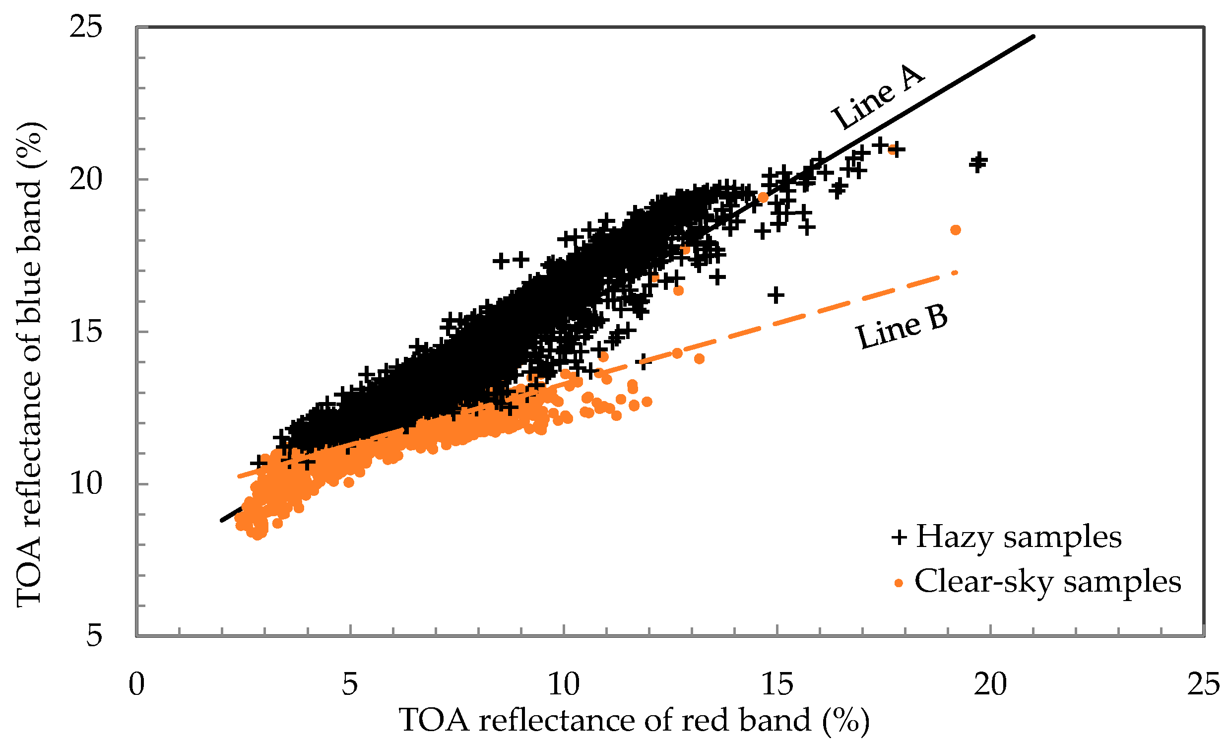
Knowing that there is normally no clear-cut boundary between hazy and haze-free zones in a scene, the goal of automating HOT is to automatically define an optimized CL that minimizes both omission and commission errors in terms of haze detection. The development of AutoHOT was started with analyzing the relation of a CL with the regression line of an entire scene. Figure 1 shows a HOT space and two scatter plots composed by samples taken separately from the hazy and haze-free regions in a Landsat-8 OLI image (Path 52/Row 16) acquired on 17 August 2014. Overall, the hazy samples are located above the clear-sky samples. The straight lines A and B in Figure 1 are the trend lines regressed from all the samples (including both hazy and haze-free samples) and the clear-sky samples only, respectively. Because of the existence of the hazy samples, the line A has been dragged away from the line B (a CL) upward at the brighter end. The line A can easily be obtained from a given scene, while the line B cannot be defined without having a number of pre-selected representative clear-sky pixels.

In Figure 1, it can be conceived that, if another linear regression is conducted over the remaining samples after eliminating the samples above the line A and with perpendicular distances bigger than a specified distance threshold (hereinafter the specified distance threshold is referred to as trimming distance and denoted by TD), then the new trend line will be closer to the line B, compared to the relation of the line A to the line B. Based on this idea, an iterative upper trimming linear regression (IUTLR) process was developed. For a given TD, an IUTLR process starts with a linear regression over all the pixels of a scene. During the next iteration, a pixel subset is first produced by excluding the pixels above the regression line obtained from the preceding iteration and with perpendicular distances bigger than the TD. Subsequently, a new linear regression is performed over the remaining pixels in the subset. This iterative process is repeated until no significant changes were observed with respect to the coefficients (slopes and intercepts) of the regression lines from two consecutive iterations. Our experiments indicated that a small number of iterations (rarely exceeding 50) usually were sufficient for an IUTLR process to converge to a steady state. In this paper, the pixel subset and its corresponding regression line created by the last iteration of a converged IUTLR process are named IUTLR pixel subset and IUTLR line, respectively.

To figure out the relationship between TD changes and their resulting IUTLR pixel subsets, IUTLR processes associated with different TDs have been applying to a number of Landsat images. Generally, the sizes of the IUTLR pixel subsets of an image are proportional to the values of the specified TDs. A close inspection to the variations of the IUTLR pixel subsets of a scene reveals that, with the increasing of the TD values, the pixel subsets normally undergo a growing process from initially including dark clear-sky pixels to the status containing most clear-sky pixels, and then incorporating some thin hazy pixels besides the clear-sky pixels. From these observations, it can be inferred that with an appropriate TD specified, it is possible to obtain an optimized IUTLR pixel subset containing a maximum number of clear-sky pixels and a minimum number of hazy pixels in a scene. Obviously, if IUTLR processes are involved in the automation of HOT, then the core of the algorithm is how to determine such an optimized TD. With an optimized IUTLR pixel subset available, an optimized CL and an optimized HOT image can be derived.

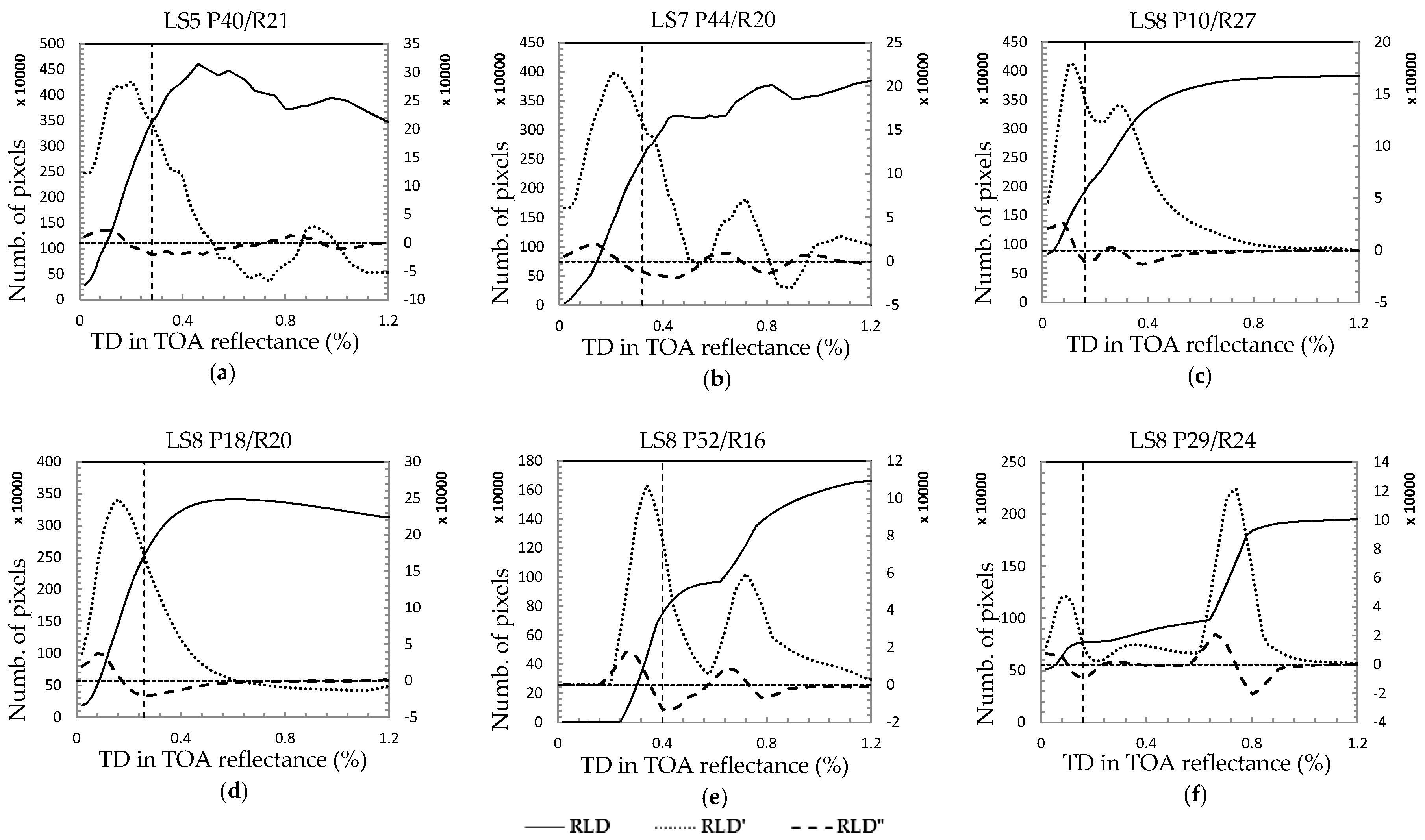
To search for an optimized TD for a scene, a double-loop scheme was introduced by nesting an IUTLR process inside the body of a loop controlled by N evenly increased TDs (the step size of the TD increment used in this study was 0.02 in the case of TOA reflectance). With this double-loop mechanism, N IUTLR lines along with N IUTLR pixel subsets can be derived for an image scene. Our strategy was to identify an optimal TD through evaluating the N IUTLR lines or N IUTLR pixel subsets. Either way, a statistical metric is needed for the evaluations. If the scatter plots of hazy and haze-free pixels in a HOT space are regarded as two classes, then the evaluations can be accomplished by measuring the separabilities of the two pixel groups separated by an IUTLR line. Unfortunately, our experiments indicated that some commonly used separability metrics, such as Jeffries–Matusita distance, Bhattacharyya distance and the transformed divergence, did not work well in this circumstance. This forced us to look for an alternative evaluation metric. According to the principle of HOT, we know that in the scatter plot of an image in HOT space, there must be a dense area composed by highly correlated clear-sky pixels. The IUTLR lines that pass through the dense scatter area should be the candidates of an optimal IUTLR line. From this analysis, regression line density (RLD) was adopted as the statistical metric for evaluating the N IUTLR lines of an image. The RLD value of an IUTLR line can be obtained by counting the number of pixels confined within a thin HOT space stripe area centered by the IUTLR line. Note that the widths of the stripe areas defined for all the IUTLR lines of a scene must be a constant small value (e.g., 0.2 in the case of TOA reflectance). By plotting the RLD values of N IUTLR lines as a function of N evenly increasing TDs, a RLD curve can be constructed for a scene. The six RLD curves (the solid curves) displayed in Figure 2 (the descriptions about the six Landsat scenes are provided in Section 2.1) are considered representative according to the smoothness of the curves and the number of local maximums.

The original purpose of creating a RLD curve for a scene was to expect there is a local maximum on the curve that corresponds to an optimized TD. This expectation apparently was found to be invalid from the inspection of Figure 2, as not every RLD curve had a local maximum (e.g., Figure 2c,e,f). Our experiments further revealed that even if a RLD curve had a maximum point; the point normally was not associated with an optimized TD. To find out a way to determine an optimized TD based on a RLD curve, a three-step experiment was undertaken over a large number of Landsat scenes (none of the scenes was included in the testing data set of this paper). First, an optimal HOT image and N IUTLR pixel subsets corresponding to N evenly increasing TDs were created separately for each of the Landsat scenes. The optimal HOT image of a scene was generated with Manual HOT using the procedure described in Section 4.1 and served as a reference case against which the N IUTLR pixel subsets were evaluated. Next, the spatial agreements between the N IUTLR pixel subsets and the clear-sky areas in the optimal HOT image of a scene were measured using overall accuracy formula, in which the hazy pixels and clear-sky pixels are treated as two classes. Finally, the IUTLR pixel subset with the best spatial agreement with the optimal HOT image of a scene was identified as an optimized IUTLR pixel subset and its corresponding TD was marked on the RLD curve of the scene. In addition to the RLD curves, the first- (RLD’) and second-order derivatives (RLD”) (e.g., the dotted and dashed curves in Figure 2, respectively) of the curves were also created and involved in the experimental analysis. Through this experiment, a general trend has been found that the locations of most identified optimized TDs were correlated with the minimum points within the first negative segment of the RLD” curves.

According to the definition of RLD, it can be understood that a peak point of a RLD’ curve must correspond to an IUTLR line in HOT space that passes through (not necessarily the center) a dense scatter plot area. For a given image, there could be one or more dense scatter plot areas in HOT space (e.g., one is formed by clear-sky pixels and another one is constituted by the hazy pixels affected by homogenous haze). According to the optical property of haze scattering (most haze types have greater impacts to blue band than to red band), it can be said that the darkest dense scatter plot area in HOT space must be clear-sky pixel scatter plot (CSPSP). Thus, the first peak point of a RLD’ curve can be used to roughly locate CSPSP. However, we must realize that the IUTLR line associated with the first peak cannot be utilized to separate the clear-sky pixels from the hazy pixels of a scene, as it passes through the CSPSP. Recalling that IURLR pixel subsets undergo an expanding process with the increasing of TD values, it can be imagined that, after the first peak of a RLD’ curve, the expanding process must have a notable slow down when it hits the boundaries between clear and haze zones of an image. Based on derivative analysis, the minimum point of the first negative segment of RLD” curve represents a significant drop on RLD’ curve, therefore can be used to estimate an optimized TD that results in an optimized IUTLR pixel subset. With the understanding and considering some special cases, the following two rules have been developed for automatically determining an optimized TD for a scene: (1) within the first negative segment of a RLD” curve, if the distance between the minimum point and the start point of the segment (equivalent to the first peak of RLD”) is smaller than a threshold (e.g., 0.2), then the TD corresponding to the minimum point can be used as the optimized TD; otherwise, (2) the optimized TD is equal to the TD value associated with the start point plus half of the threshold. The optimized TDs in Figure 2a,c–f were determined using the first rule, while the optimized TD in Figure 2b was detected based on the second rule.

3.3. HOT Image Post-Processing

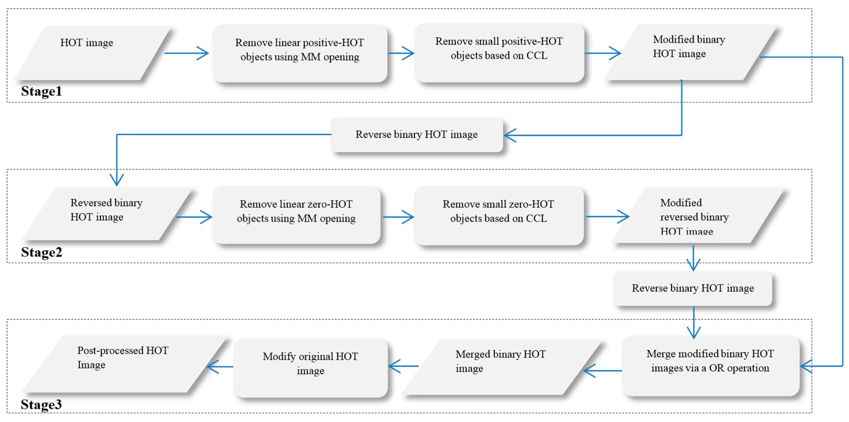
Since the HOT values of the pixels below a CL are set to zero, a HOT image consists of a set of connected positive-HOT and zero-HOT image regions. Due to spurious HOT responses, the HOT values of some pixels do not reflect their haze conditions (e.g., clear-high-HOT and haze-zero-HOT situations). To reduce the influences of spurious HOT responses to haze removal, AutoHOT includes two additional steps, HOT image post-processing and class-based HRA. HOT image post-processing was developed based on an assumption that haze regions normally occur over large spatial scales. Thereby, fine-scale (either with small areas or with thin linear shapes) positive-HOT and zero-HOT objects most likely result from spurious HOT responses and should be removed from a HOT image.

Figure 3 depicts the flowchart of HOT image post-processing. The procedure can be generally divided into three stages. The first two stages are designed to identify fine-scale clear-high-HOT and haze-zero-HOT objects in HOT images, respectively. The algorithms used in these two stages are implemented with the help of the opening operation of mathematical morphology [29] and connected component labeling [30]. The results of the first two stages are stored separately in two binary images. In the third stage, the two binary image are first merged via a logical OR operation. In the merged binary image, the pixels with 0 or 1 represent clear-sky or hazy pixels, respectively. The second step of the third stage is to modify the original HOT image according to the following two rules: (1) change a positive HOT value in the HOT image to zero if its corresponding pixel in the merged image is zero; and (2) estimate a HOT value for a zero-value pixel in the HOT image if its corresponding pixel in the merged image is one. The HOT value estimation currently is done using spatial interpolation with inverse distance weighting.

3.4. Class-Based HOT Radiometric Adjustment

HOT image post-processing only reduces the number of two types of spurious HOT responses, clear-high-HOT and haze-zero-HOT. To minimize the haze compensation errors due to haze-high-HOT, haze-low-HOT and inconsistent dark targets are present under different haze conditions (violation of the assumptions of HRA, see Section 3.1.5), an improved version of HRA was developed for AutoHOT by applying HRA to each classified pixel group (hereinafter the improved HRA is referred to as class-based HRA).

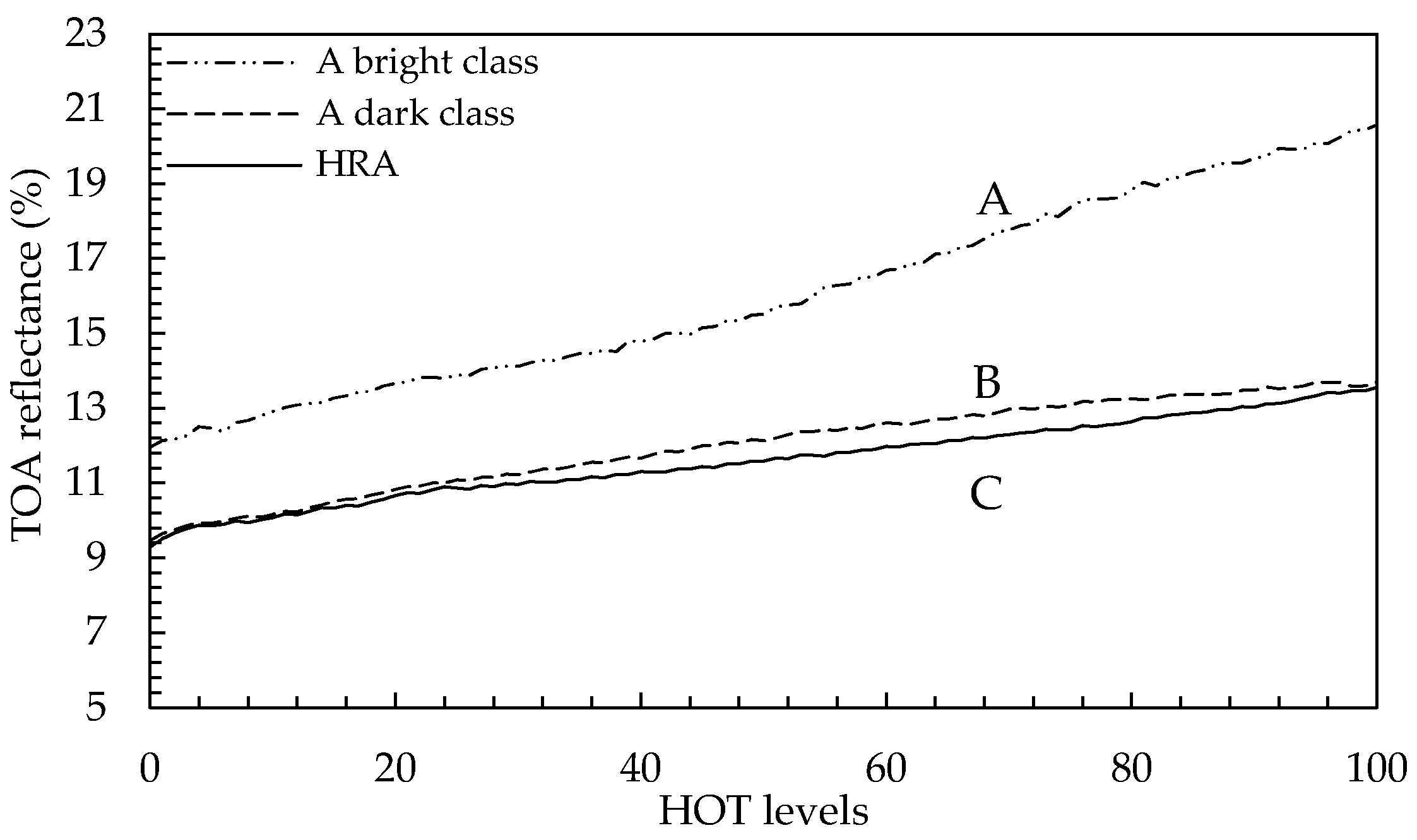
For illustrating the necessity of applying class-based HRA, three dark-bound mean curves of 100 HOT levels (HOT value ranged from 0.0 to 5.0 with a step size equal to 0.05), shown in Figure 4, were generated using the first (coastal/aerosol) band of a Landsat-8 OLI scene (Path 50/Row 25, mainly water and mountainous areas) acquired on 19 August 2014. Lines A and B in Figure 4 are generated with dark-bound means of a bright class (mainly deforestation areas) and a dark class (dominated by shadow and shade pixels of mountains), respectively. Line C (in Figure 4) was created in the same way as in conventional HRA with the dark-bound means of different HOT levels regardless land-cover types. It can be understood that, for the hazy pixels of the dark class, two HOT-based haze removal methods will produce similar results. Because the overall slopes of line B (the base line for correcting the dark class in class-based HRA) and line C (the base line for correcting all hazy pixels in conventional HRA) are very close, conventional HRA will undercompensate the hazy pixels of the bright class, since the slope of line A is much bigger than that of line C. It must be pointed out that the notable slope difference between line A and C is not fortuitous, the difference is consistent with the results obtained from the MODTRAN-based haze effect simulation conducted by Zhang et al. [6]. This means that class-based HRA conforms more accurately to the outputs of atmospheric radiative transfer model.

In class-based HRA, the class-dependent HOT values are employed in the haze compensation of similar surface type. This ensures that the HOT values involved in the calculation mainly reflect atmospheric haze intensities, rather than the variations of surface reflectance; therefore, the first HRA assumption is automatically satisfied. A requirement of applying class-based HRA is the existence of a set of clear-sky pixels for every class. In this study, the minimum number of clear-sky pixels for each class was set to 1000 for statistical representation. If a class does not have a sufficient number of clear-sky pixels (rarely happen in our study), then some dark clear-sky pixels of a class most similar to the targeted class are employed as supplements. The worst scenario of class-based HRA is that none of the classes has an adequate number of clear-sky pixels. In this case, conventional HRA can be applied. It is worth mentioning that HOT image post-processing is a helpful step for class-based HRA, because it can remove fine-scale clear-high-HOT objects from a HOT image. This could be critical for applying class-based HRA to some land-cover types such as man-made targets and bare rock/soil. Because these surface types might not have a sufficient number of clear-sky pixels without HOT image post-processing. On the other hand, class-based HRA ensures that the darkest pixels used for estimating the radiometric adjustments for different HOT levels of a class more likely belong to the same (or similar) land-cover type, meaning that the second assumption of HRA can be met to some degree as well.

Obviously, a classification map must be available to apply class-based HRA. With the intention of fully automating AutoHOT, we adopted the idea suggested by Liang et al. [16] for unsupervised classification with haze-transparent bands (bands 4, 5 and 7 in the case of Landsat sensors 5 and 7; bands 5–7 in the case of Landsat 8). To increase the computational efficiency, a K-mean clustering analysis was applied to a number (normally a few hundreds and thousands) of the samplers created by a spectral screening process [31], rather than to an entire scene. To ensure that the histogram of each land-cover class is formed with large pixel populations, a small number (5 to 10) of classes had been specified in the classification. Note that the number of the classes used for class-based HRA does not necessarily match the actual number of the land-cover classes exhibit in a scene, because the purpose of the classification here is to roughly divide the scene pixels into a few groups, particularly to separate brighter classes from darker classes, rather than the classification in traditional sense.

4. Experiments and Analysis

Because of the spatiotemporal variations of atmospheric haze conditions and the extreme difficulties of collecting spatially detailed in-situ haze measurements during each satellite overflight, a realistic approach for evaluating a haze removal method is to rely on the image scene itself. In this section, the performances of AutoHOT in haze detection and correction were assessed through three experiments with ten selected Landsat scenes that cover diverse Canadian landscapes and atmospheric haze conditions (see Table 1). The goal of the experiments was to demonstrate that AutoHOT for haze removal is not only efficient, but also robust and effective. The first experiment described in Section 4.1 is to examine the spatial agreements between the HOT images created with AutoHOT and Manual HOT for nine selected Landsat scenes. In Section 4.2, the second experiment is presented to prove the correctness of the HOT image from AutoHOT with a pair of hazy and haze-free Landsat scenes of the same site. Finally, the advantage of class-based HRA over conventional HRA is demonstrated in Section 4.3 with the third experiment, in which nine of the ten selected Landsat scenes were involved.

4.1. Experiment 1: Spatial Agreement between HOT Images

This experiment was carried out to quantitatively and visually examine the spatial agreement between the HOT images created with AutoHOT and Manual HOT. The goal of the experiment was to demonstrate that IUTLR-based fully automated HOT can not only identify clear-sky pixels efficiently, but also create HOT images that have high spatial agreement with the optimized manual HOT results.

The experiment started with applying the two HOT processes to each of the nine selected Landsat scenes (Landsat-8 OLI scene, Path 29/Row 24, acquired on 16 August 2014 was not involved in this experiment since it is an almost clear scene). Since the HOT images created with Manual HOT will be employed as the references for evaluating the accuracy of AutoHOT in haze detection, an optimized HOT image must be created with Manual HOT. As mentioned in Section 3.1.1, a large number of diverse HOT images can be created for a given scene by manually selecting different clear-sky pixel subsets. In this research, the HOT image created based on a CL defined with a maximized clear-sky pixel set of a scene was used as an optimized HOT image. Due to the complexities of the distributions of thick clouds and/or the ambiguous boundaries between the hazy and clear-sky areas in a scene, it is time-consuming to create a maximized clear-sky pixel set. For efficiency and quality purposes, the maximized clear-sky pixel set for each scene were created by following the steps described as follows: (1) Create a thick cloud mask using the algorithm reported by Zhu and Woodcock [7]. (2) Manually delineate polygons that include as many as possible of clear-sky pixels by ignoring the inclusions of thick cloud pixels. (3) Automatically remove thick cloud pixels from the polygons in accordance with the thick cloud mask.

Before calculating the spatial agreements between the HOT images created with AutoHOT and Manual HOT, a HOT image post-processing process described in Section 3.3 was applied to every HOT image. Figure 5 illustrates the effectiveness of HOT image post-processing for a sub-scene clipped from Landsat-8 OLI image (Path 19/Row 30) acquired on 26 August 2014. In the HOT image before post-processing (Figure 5b), various spurious HOT responses can be easily observed. For example, the linear road and soil land positive-HOT features in clear-sky areas (left side of the sub-scene) represent clear-high HOT, the holes (zero-HOT features) within hazy areas (right side of the sub-scene) are haze-zero-HOT. From Figure 5c, it can be seen that most linear clear-high-HOT features have been removed, while some relatively big soil land positive-HOT features still remain in the HOT image after post-processing. Moreover, some holes within hazy areas have been filled by post-processing.

In this study, the spatial agreements were measured with overall, user’s and producer’s accuracies by regarding the hazy pixels (with positive HOT values) and haze-free pixels (with zero HOT values) in a HOT image as two classes.

Table 2. Spatial agreement accuracies between the HOT images created with AutoHOT and Manual HOT for nine selected Landsat scenes (sorted by overall accuracies). A_overall, A_user and A_producer are overall, user’s and producer’s accuracies.

WRS	Aoverall	Auser	Aproducer
Path 40/Row 21	0.891	0.931	0.873
Path 10/Row 27	0.951	0.999	0.948
Path 18/Row 20	0.959	0.948	0.999
Path 44/Row 20	0.960	0.949	0.999
Path 61/Row 16	0.970	0.977	0.991
Path 50/Row 25	0.979	0.993	0.985
Path 19/Row 30	0.983	0.989	0.993
Path 52/Row 16	0.991	0.997	0.994
Path 29/Row 24	0.996	0.999	0.996

lists the agreement accuracies between the HOT images created with the two HOT processes for nine Landsat scenes. The relative lower accuracies associated with the Landsat-5 TM scene could be caused by its lower radiometric resolution, which results in its RLD curve bumpier (Figure 2a). The average overall, haze user’s and producer’s accuracies are 96.4%, 97.6% and 97.5%, respectively. This confirms that, under a variety of landscapes and atmospheric haze conditions, automated HOT can effectively detect hazy pixels as the best of Manual HOT can do. With further inspection of Table 2, no notable trend can be seen among the three accuracy measures, meaning that AutoHOT does not have a significant bias for overestimating or underestimating hazy pixels. Figure 6 displays the true color and the HOT images of the four Landsat scenes with lower overall accuracies. Visually, both AutoHOT and Manual HOT can effectively detect hazy pixels and the spatial patterns of the detected hazy areas in corresponding HOT images are quite similar.

4.2. Experiment 2: Correctness of HOT Image from AutoHOT

An accurate haze intensity map (equivalently the HOT image in HOT-based method) is the basis of successfully removing haze effects from a visible band. Based on a pair of hazy and almost haze-free Landsat-8 OLI scenes over the same geographic region (Path 29/Row 24), the second experiment was undertaken to visually and quantitatively prove the correctness of the HOT image produced by AutoHOT. The paired scenes were acquired separately on 31 July (hazy scene) and 26 August (reference clear scene) 2014. About 97% of the hazy scene is covered by thin cloud and/or haze. While only a small portion of the left side of the reference scene is affected by thin haze. Figure 7 illustrates the image comparisons between the sub-scenes clipped from the hazy, dehazed (using class-based HRA) and reference scenes. From a visual interpretation of the sub-scenes, it can be confirmed that the reflectance features of various land-cover surfaces have been properly restored by AutoHOT.

To quantitatively assess the correctness of the HOT image from AutoHOT, the histograms and the correlation coefficients were created for the four visible bands of the three images (hazy, dehazed and reference). Figure 8 illustrates the histogram comparisons of the three images in four visible bands. Each of the four histograms (short-dashed curves) of the reference scene has only one peak and should be regarded as the typical histogram shape of each visible band. There are two peaks on each of the four histograms (long-dashed curves) of the hazy scene. The right and left peaks correspond to the large hazy area and the small clear-sky area in the hazy scene. Each of the four histograms (solid curves) of the dehazed scene has only one peak and is very consistent with the shape of its corresponding histogram of the reference scene. This histogram comparison demonstrates that the radiometric values of the hazy pixels in the hazy scene have been normalized close to the radiometric level of the clear-sky pixels in the same scene. The constant shifts between the histograms of the reference and the dehazed images could be due to the resistance of class-based HRA to haze overcompensation.

Figure 9 shows the scatter plots and linear regression lines between the samples taken from the hazy (crosses) and dehazed (dots) versus the corresponding samples taken from the reference images of four visible bands. To create these samples, an unsupervised classification on the clear-sky pixels in the reference scene was first carried out with seven optical bands of Landsat 8 OLI data. The classification map was employed as the definitions of the homogenous areas for calculating the mean values of different surface types in four visible bands of the three images (hazy, dehazed and reference). Since 100 classes have been specified in the classification, each scattergram is composed of 100 samples. As about 97% of the pixels in the hazy scene are contaminated by thin cloud or haze, every class of the hazy scene is dominated by hazy pixels. This is why every sample from the hazy scene seems to have been corrected by AutoHOT. From the four pairs of the scatter plots in Figure 9, it can be seen that the correlation coefficients between reference samples and their corresponding hazy samples increase with the increasing wavelengths of the bands. This trend agrees with the optical properties (scattering effect is inversely proportional to the increase of wavelength) of most aerosol types [5]. The regression coefficients of the four visible bands are improved from 0.441, 0.535, 0.794 and 0.902 before haze correction to 0.762, 0.846, 0.902 and 0.945 after haze correction, respectively. It is worth noting that the results of this experiment demonstrate not only the correctness of the HOT images created with AutoHOT, but also the performance of class-based HRA.

4.3. Experiment 3: Advantage of Class-Based HRA

Besides automating HOT, AutoHOT also improves HRA by combining HRA with classified pixel groups. Although experiment 2 implicitly demonstrated the performance of class-based HRA, it is necessary to explicitly illustrate the improvement through a separate experiment. This experiment was designed based on the assumption that haze correction should reduce the differences between the mean values of the hazy and haze-free pixels of the same land-cover class. The nine Landsat scenes listed in Table 2 are employed in this experiment. With a rough interpretation to the scenes, eight classes were specified for classifying all the test scenes. As discussed in Section 3.4, this number of classes is appropriate for class-based HRA, even if it may not match the actual number of the surface classes in some scenes. To ensure the two HRA methods are compared on the same basis, only the HOT images produced with AutoHOT were used in this experiment. After applying the two HRA methods, two dehazed images were created for each scene. Thus, there are three images associated with each Landsat scene and they are the original, dehazed with class-based HRA and dehazed with conventional HRA. With a HOT image and a classification map available for a scene, four mean values (mean of clear-sky pixels, mean of original hazy pixels, mean of dehazed pixels with class-based HRA and mean of dehazed pixels with conventional HRA) of a class (c) in a band can be calculated. For simplicity, these mean values are symbolized as by$m_{clear}^c$,$m_{hazy}^c$, $m_{classHRA}^c$ and $m_{HRA}^c$, respectively.

Figure 10 illustrates the comparisons of the four mean values of all the classes in the nine Landsat scenes. The mean values were calculated based on the pixels in the first band (blue band in the case of Landsat sensors 5 and 7; coastal/aerosol band in the case of Landsat 8) of the three image sets of each scene. In Figure 10, it can be clearly seen that both class-based HRA and conventional HRA reduce the differences between $m_{hazy}^c$ and $m_{clear}^c$ to varying degrees. A closer inspection of Figure 10 reveals that the difference between $m_{classHRA}^c$ and $m_{clear}^c$ is smaller than that between $m_{HRA}^c$ and $m_{clear}^c$ for most classes in most scenes. This illustrates that class-based HRA can create better dehazed results than conventional HRA. Additionally, it has been noted that class-based HRA shows significant improvements for some brighter classes, while has similar performances as conventional HRA for darker classes. This is because class-based HRA has the ability of overcoming the dependence of HOT on surface reflectance. In Figure 10a,h, it can be found that conventional HRA overcompensates the haze effects for most classes in Path 40/Row 21 and Path 52/Row 16 scenes.

5. Conclusions

A fully automated and robust haze removal method is an essential requirement for remote sensing applications involving a large volume of optical images. After reviewing and analyzing the concepts and major issues related to Haze Optimized Transformation (HOT)-based haze removal, a methodology named AutoHOT has been developed in this study to fully automate HOT process and improve the accuracy of HOT-based haze removal. AutoHOT is composed of three steps covering various aspects of a haze removal task. The innovations introduced in AutoHOT include iterative upper trimming linear regression, HOT automation based on derivative analysis, novel HOT image post-processing and class-based HOT radiometric adjustment (HRA). In addition to algorithm development, the principles of the algorithm (HOT automation and class-based HRA) have also been analyzed in detail. These analyses establish the foundation of AutoHOT and ensure its generality. The performances of AutoHOT in haze detection and correction were evaluated through three experiments with ten selected Landsat scenes. The results of the experiments demonstrated that AutoHOT is robust and effective for the scenes acquired over various Canadian landscapes under diverse atmospheric haze conditions, and can automatically produce more accurate dehazed images than Manual HOT. From this research, the following conclusions can be drawn.

• AutoHOT can not only fully automate HOT, but also create an optimized HOT image by defining an optimized clear line with a maximum set of clear-sky pixels exhibit in a scene.
• It is important to categorize spurious HOT responses according to their radiometric features in a HOT image. The categorization has helped us in the development of different strategies for addressing the issue. At present, the impacts of most spurious surfaces to a HOT image can be reduced either by HOT image post-processing or class-based HRA components of AutoHOT. This implies that AutoHOT can relax the requirement to the correlation of clear-sky pixels in HOT space.
• Even though class-based HRA can increase the accuracy of haze removal, it is still a relative radiometric correction. Further research is needed to investigate the possibility of utilizing a HOT image in an absolute radiometric correction; for example, how to incorporate a HOT image into the process of an atmospheric correction based on a radiative transfer model.
• AutoHOT was developed for removing haze effects from Landsat imagery. However, since only two visible bands are needed, it is possible to extend the method to the images acquired by other optical remote sensing systems that include blue and red channels. Of course, if an image does not have haze-transparent bands, then a classification map cannot be derived from the image itself. This means that class-based HRA could be limited if there is no other way to get a latest classification map for the images under investigation. Another issue related to applying AutoHOT to other optical remotely sensed imagery is the impact of image spatial resolution to HOT. The lower the image spatial resolution is, the more mixed pixels could be present in the image. It will be interesting to find out whether or not HOT can be affected by image spatial resolutions.