1. Introduction
Carbon dioxide, one of the greenhouse gases, has significantly increased since the industrial revolution due to economic and population growth. Increase of carbon dioxide concentration in the atmosphere accelerates global warming, which is directly related with on-going climate change. Climate change has brought significant impacts on human society and the natural environment all over the world, in such ways as increasing extreme weather events and a rise in sea levels [
1]. The ocean contains fifty times more carbon dioxide than the atmosphere, and twenty times more than terrestrial ecosystems. Although the substantial amount of carbon dioxide in the atmosphere is absorbed into the oceans, approximately half of anthropogenic carbon dioxide remains in the atmosphere, increasing its concentration [
2]. Since the ocean acts as a buffer for carbon dioxide uptake, temporal and spatial changes of the sea-air carbon dioxide flux are crucial to understanding the global carbon cycle [
3].
The increasing absorption of carbon dioxide from the atmosphere can result in huge damage to marine organisms [
4]. When the carbon dioxide dissolves in seawater, it becomes carbonic acid and has a negative effect on biochemical functions of organisms, in particular, calcareous ones, such as lime, coral algae, clams, and oysters, with their shells composed of calcium carbonate ([
5] and references therein, for example). Accumulated carbon dioxide in the ocean accelerates global warming and climate change by decreasing the capacity of the ocean that absorbs carbon dioxide from the atmosphere. Consequently, quantifying the distribution of ocean carbon dioxide is crucial in order to better understand the ocean carbon sink [
6]. However, there has been limited exploration of ocean carbon dioxide around East Asia, especially in the East Sea located between Korea and Japan.
In situ field observations are relatively limited over the ocean because of technical and financial problems [
6]. In addition, in situ measurements are not typically continuous in the spatiotemporal domain. Satellite remote sensing can be a good alternative to this as satellite sensors collect data over vast areas at high temporal resolution (~hours). Satellite data can be used to estimate various ocean parameters including chlorophyll-a concentration (Chl-a), sea surface temperature (SST), and colored dissolved organic materials (CDOM), which are related to the distribution of carbon dioxide in the ocean.
In this study, we used multi-sensor satellite data and in situ measurements to quantify carbon dioxide over the East Sea of Korea. This study focuses on the fugacity of carbon dioxide (ƒCO
2) in surface seawater, in order to examine ocean carbon dioxide. Fugacity is expressed in Pascals or in atmospheres, the same unit as is used with partial pressure. Since it is difficult to retrieve pressure (or fugacity) of carbon dioxide directly from satellite reflectance data, it is necessary to use satellite-derived ocean parameters that are related to carbon dioxide concentration [
7]. Many studies have suggested that SST and Chl-a are the important parameters for estimating the partial pressure of carbon dioxide [
8,
9,
10,
11,
12,
13,
14,
15,
16,
17,
18,
19]. The capacity of gas solubility is highly related to SST. SST also affects other carbon pumps, which are physical transport and biological photosynthesis and respiration [
20]. SST could act as an indication of cooler upwelling water by vertical mixing [
7]. In addition, sea surface salinity (SSS) [
6,
7,
8,
11,
12,
15], mixed layer depth (MLD) [
10,
11,
16], CDOM [
21], and wind speed [
6,
16,
21] were used to quantify the partial pressure of carbon dioxide in the ocean. SSS also shows the variability of carbon dioxide by expressing the mixing between seawater and freshwater [
7]. SSS can determine the characteristics of surface seawater carbon dioxide not determined by other ocean parameters (i.e., SST, MLD, and biological variables) as water mass tracer and water parcel history [
22]. MLD is defined as the depth of the vertical mixing process of the ocean. The bottom layer of seawater has a high concentration of dissolved inorganic carbon, which can come up to the surface through the process, resulting in ƒCO
2 increases [
23,
24]. CDOM and Chl-a are controlled by organisms that produce O
2 and consume CO
2. Active photosynthesis decreases surface water ƒCO
2 [
23,
25,
26,
27]. Temperature is related to seasonal thermal balance [
7].
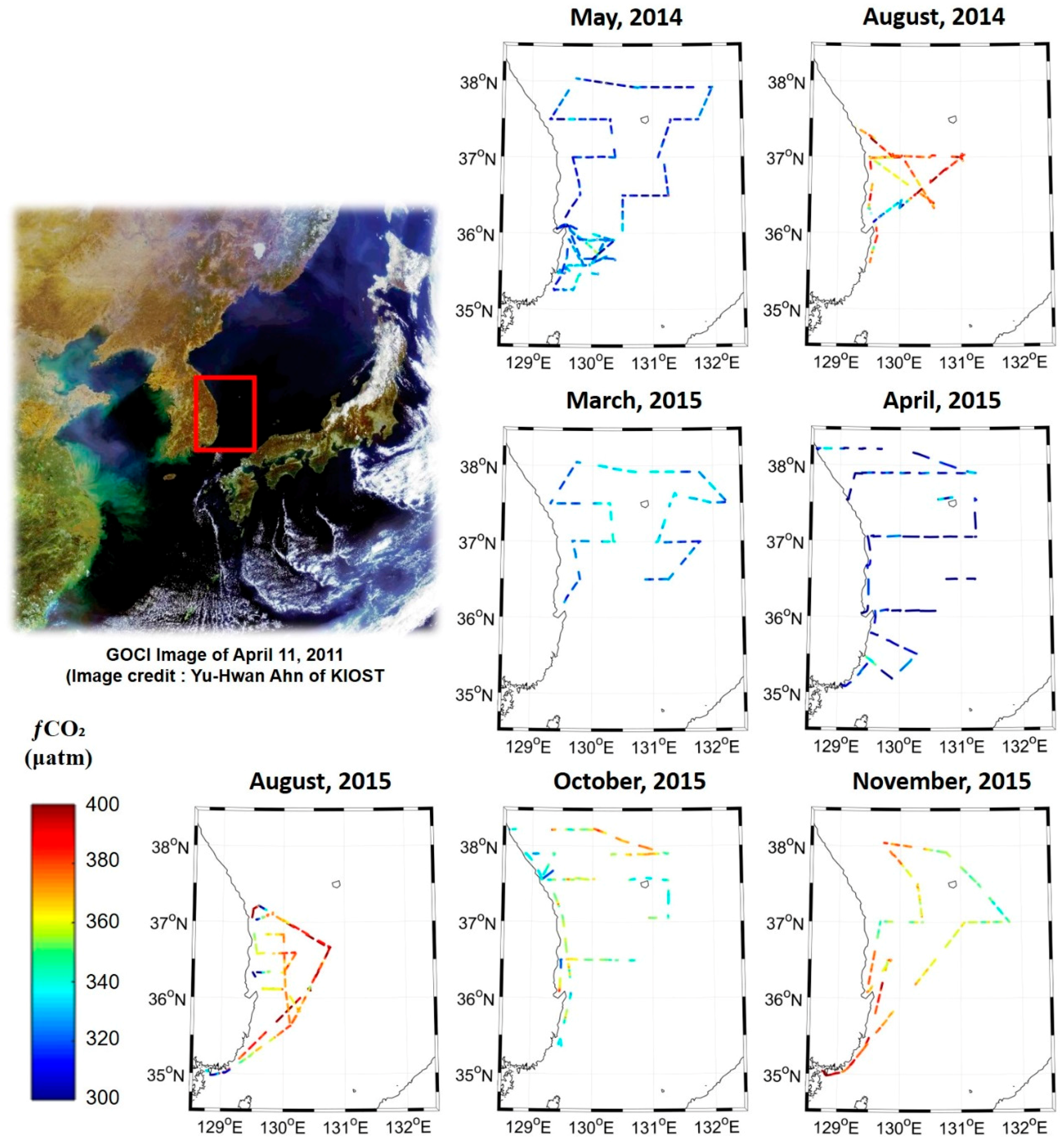
The East Sea, surrounded by Korean peninsula, Japan, and Russia, is a mid-latitude marginal sea with average depth of about 1750 m. It is connected to the western North Pacific through the Korea, Tsugaru, Soya/La Pérouse, and Tatar Straits. The inflow through the Korea Strait that brings warm and salty water, and the outflow through the Tsugaru, Soya/La Pérouse are mainly confined to about upper 150 m. Below the upper level, there is a thermohaline circulation due to deep convection occurring in the northern part of East Sea [
28,
29]. Deep convection carries anthropogenic carbon dioxide into the East Sea, making a large reservoir for carbon dioxide. The specific column inventory of anthropogenic carbon dioxide in the East Sea is two or three times greater than that of the North Pacific, which results in a great change in the carbonate chemistry of the sea through the large accumulation of carbon dioxide [
23]. Within the East Sea, ƒCO
2 varies even over a small area due to environmental variations [
30]. In response to the increase in the atmospheric CO
2 concentration, ƒCO
2 in the East Sea steadily increased between 1995 and 2010 [
20]. A numerical model with ocean carbon chemistry suggests that the inflow into the East Sea could also contribute to a change in ƒCO
2 [
31]. Considering these environments, quantifying ƒCO
2 is crucial for monitoring carbon flux in the East Sea and improving our understanding of the regional carbon cycle. However, there have been only a few studies analyzing the carbon dioxide in the East Sea using in situ data [
20,
23,
30]. Park et al. [
32] constructed a neural network model to estimate
pCO
2 in the East Sea based on satellite-derived SST and Chl-a and in situ
pCO
2 data from 2003 to 2012. The variability of
pCO
2 was large due to high primary production and mesoscale eddies, and the relationship between
pCO
2 and SST was higher than Chl-a [
32].
Most of the studies mentioned above estimated the pressure of ocean carbon dioxide using in situ and satellite data through statistical approaches, such as simple linear and multiple linear regression. Such linear approaches might not work well for the nonlinear behavior of carbon dioxide over the ocean with a dynamic spatiotemporal environment. More advanced algorithms that can handle the nonlinear behavior are required to examine the relationship between ocean carbon dioxide and ocean related parameters [
33]. In the field of remote sensing, recently adopted machine learning approaches or nonlinear analyses, may be able to effectively model the pressure of ocean carbon dioxide. These techniques include various neural networks including self-organizing maps (SOM) [
6,
14,
15,
20,
32,
34,
35], mechanistic nonlinear models [
13], principal component analysis [
9], mechanistic semi-analytic algorithms [
7], and quadratic polynomial regression [
9]. However, generalization of the empirical modeling approaches from one area to different areas is still challenging.
Most of the studies mentioned above used polar orbiting satellite sensors (especially, Moderate Resolution Imaging Spectroradiometer (MODIS)). We used Geostationary Ocean Color Imager (GOCI) satellite sensor, which has higher spatial and temporal resolutions than MODIS. This is the first study to estimate the surface seawater ƒCO2 using GOCI satellite data.
The objectives of this study were (1) to estimate surface seawater ƒCO
2 in the East Sea of Korea using satellite data and in situ measurements based on multi-variate nonlinear regression (MNR) and machine learning approaches, and (2) to examine ocean parameters contributing to ƒCO
2 estimation, and (3) investigate the spatial and temporal variation of surface seawater ƒCO
2 and sea-air CO
2 flux over the East Sea using satellite data. Two machine learning approaches including support vector regression (SVR) and random forest (RF) were used in this study. MNR, recently applied in a study [
9] to estimate
pCO
2, was used for comparison with the two machine learning approaches.
5. Conclusions
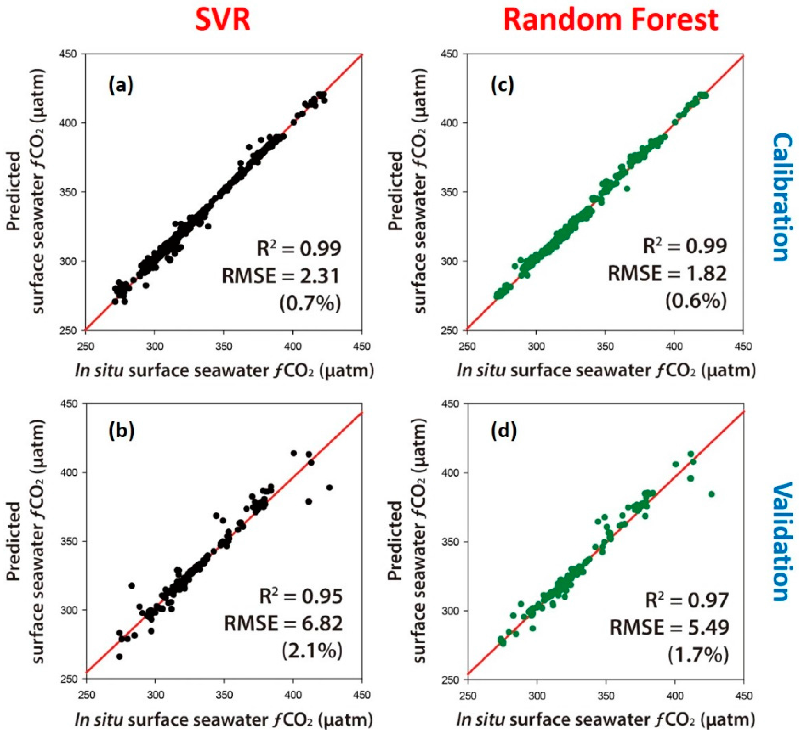
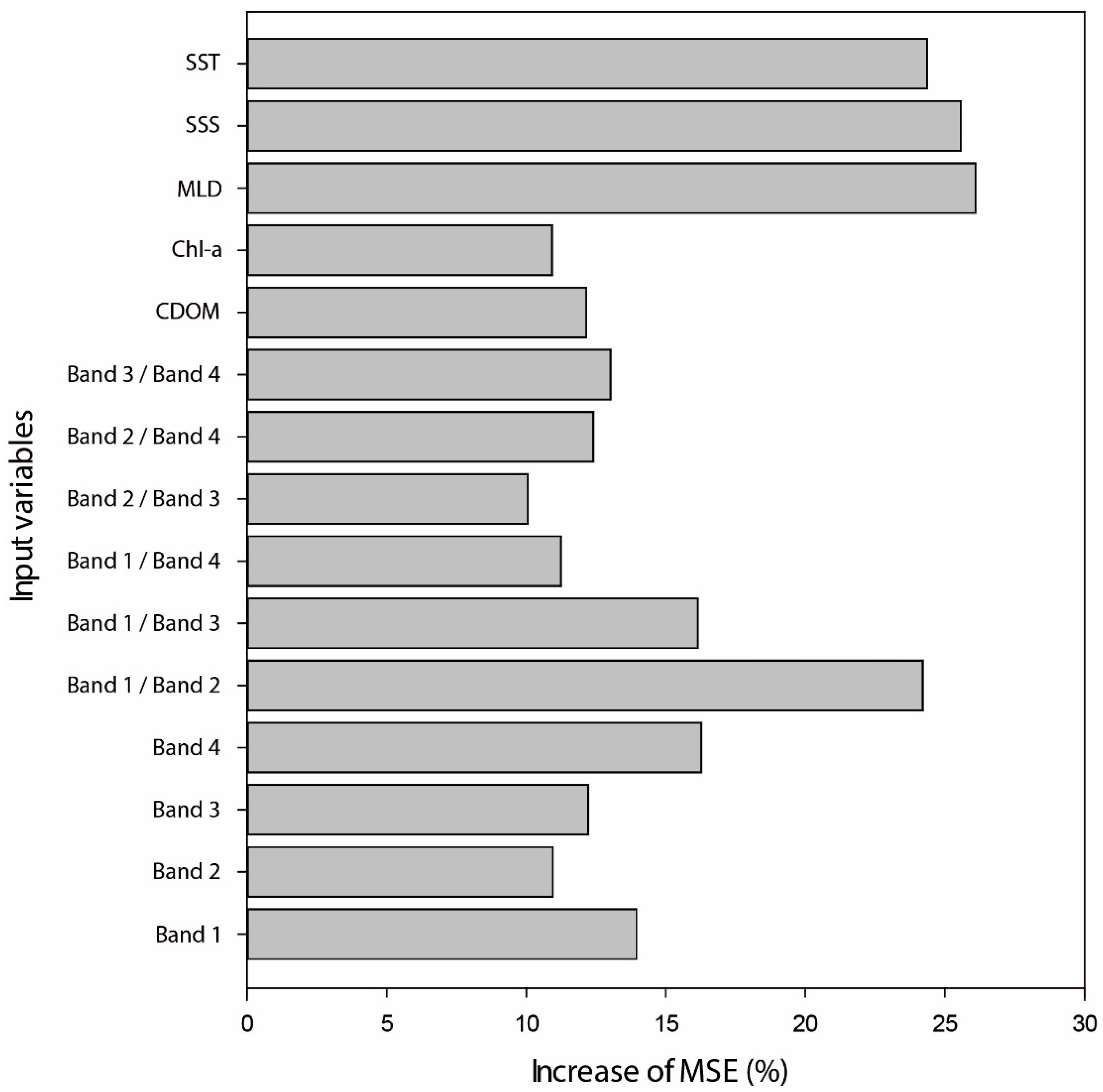
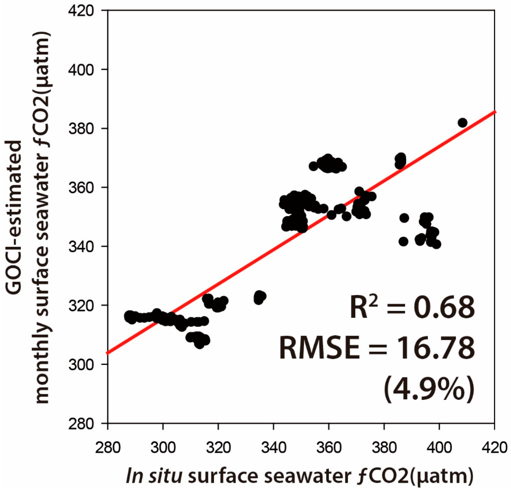
This study estimated the surface seawater ƒCO2 in the East Sea of Korea using in situ measurements, GOCI satellite and their derived products, and HYCOM reanalysis data through MNR and two machine learning approaches (RF and SVR). Results show that RF generally produced a better performance than MNR and SVR. RF effectively modeled both linear and nonlinear characteristics of surface seawater ƒCO2 through an ensemble approach. Ocean parameters (i.e., SSS, SST, and MLD) appeared to be more contributing than the individual bands or band ratios from the satellite data. Since MLD controls the amount of carbon dioxide moving into the surface from the subsurface, it may be very useful for estimating surface seawater ƒCO2. It should be noted, however, that HYCOM MLD uses a fixed threshold of change in the vertical profile of temperature to identify the depth.
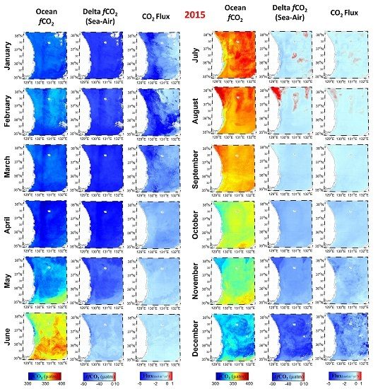
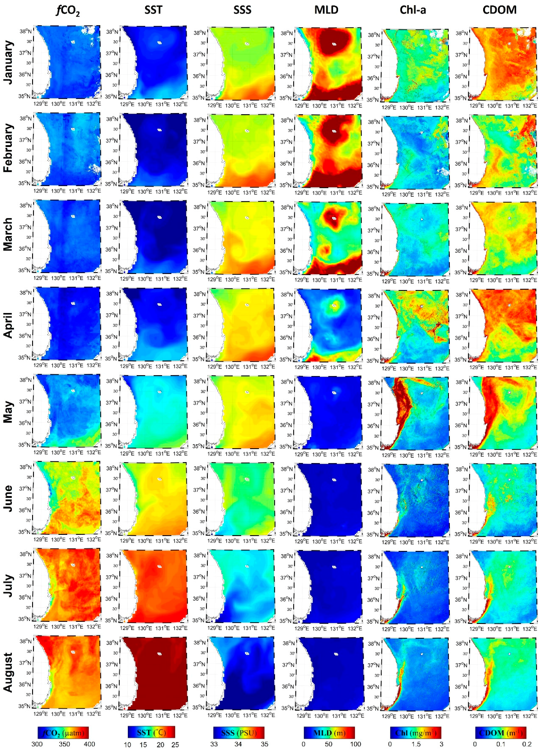
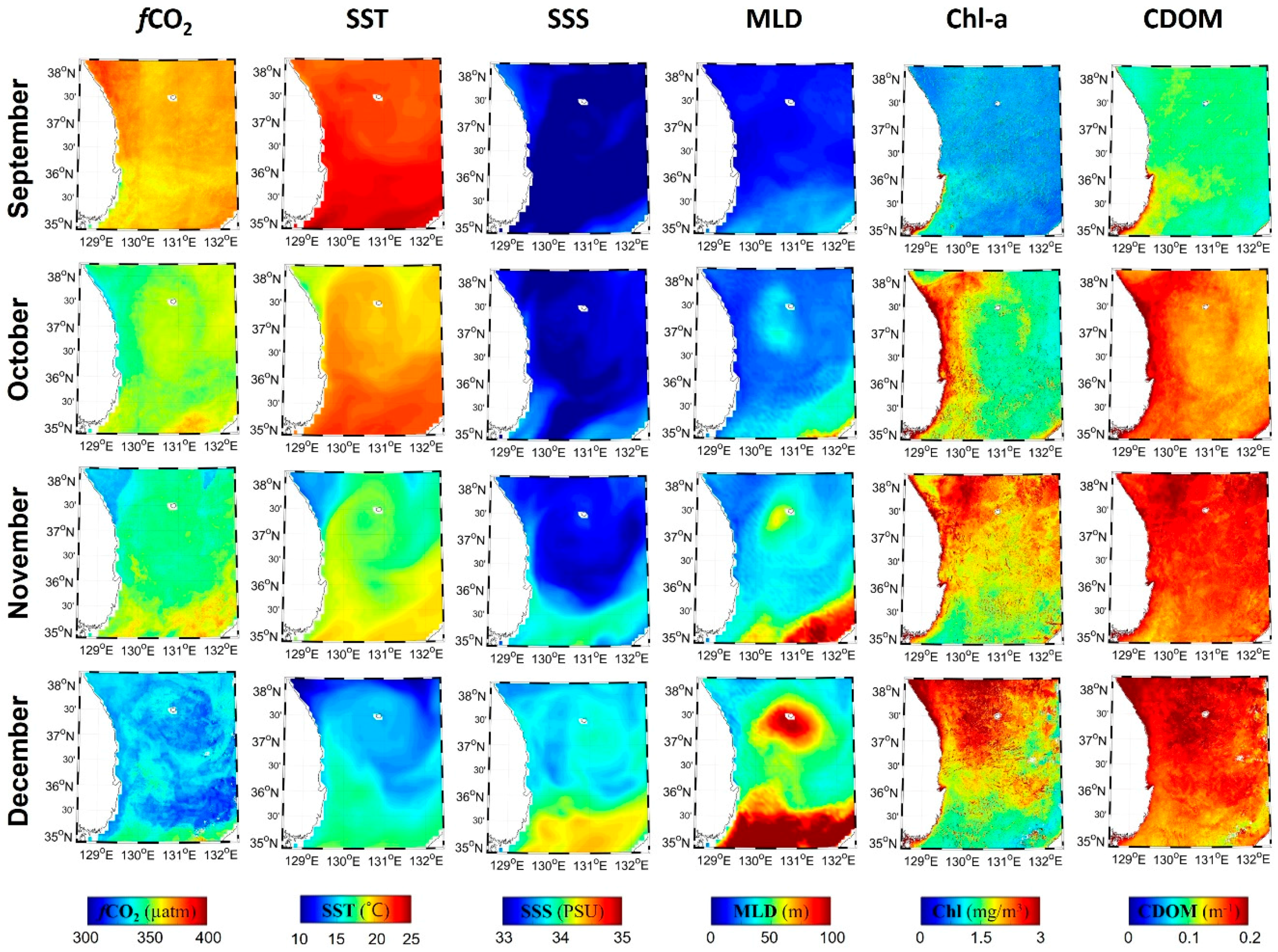
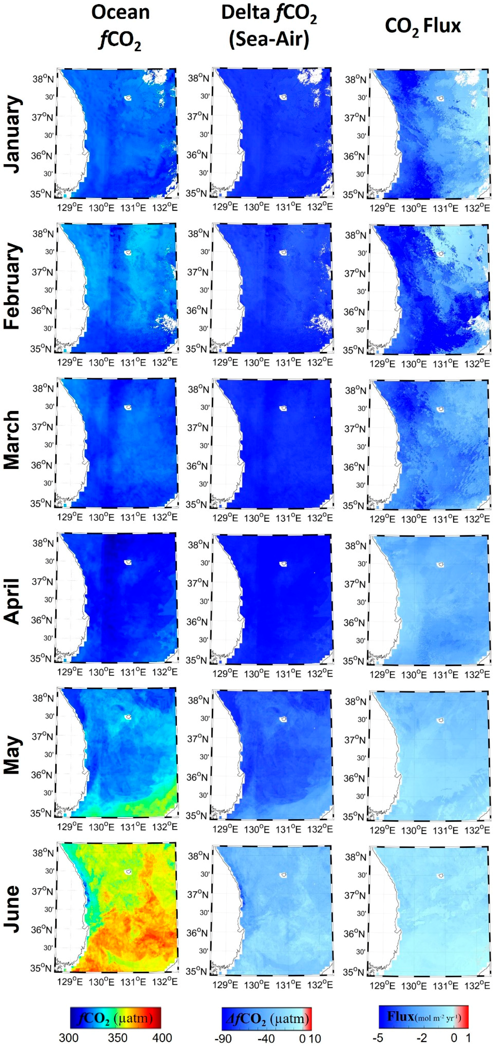
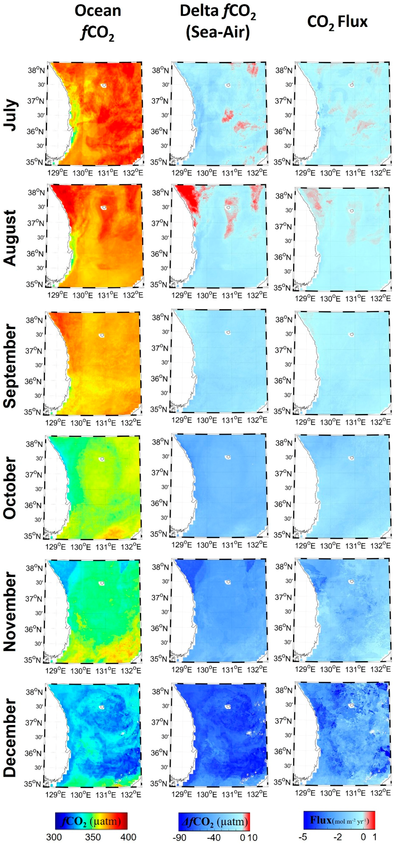
The monthly surface seawater ƒCO
2 maps in 2015 provided valuable information of seasonal spatial variations of surface seawater ƒCO
2 in the East Sea. Strong saturations of CO
2 in the ocean was observed in summer because of increased SST. Surface seawater ƒCO
2 was higher in fall than spring because of a higher SST and deeper MLD [
20]. The spatial distribution of surface seawater ƒCO
2 in the East Sea showed a strong link with SST, SSS, and MLD in GOCI-based estimation. Overall, the East Sea is a sink for atmospheric CO
2, although some areas in summer act as a weak CO2 source.
Compared to the existing literature that used traditional regression models [
8,
10,
11,
12,
16,
17,
19], this study estimated surface seawater ƒCO
2 with complicated, but more advanced algorithms than conventional statistical ones, using two machine learning approaches. In addition, using the world first geostationary ocean color satellite data (i.e., GOCI), we were able to improve the model performance: much more data collection by GOCI allowed us to use more samples temporally matched between in situ measurements and satellite-derived data. However, there are several limitations of this study, for which further research is needed. In situ measurements data used in this study only cover a few months in spring, summer, and fall. Longer time series data should be investigated to make the model much more robust and reliable. Uncertainty of satellite-derived products should also be reduced, especially near the coastal areas.


