1. Introduction
Recently, viscoelastic models have been proposed to give an account of the dissipative behaviour of the electroelastic materials [
1,
2,
3,
4,
5,
6,
7,
8,
9,
10,
11,
12]. This is justified because the range of temperatures at which these materials are being currently used is close to the glass transition temperature. Indeed, above the glass transition temperature, the materials in a rubber-like state still exhibit some rest of the viscoelastic behaviour. As a consequence, in these materials, the response to an external mechanical or electrical force field implies relaxation processes towards a new state of thermodynamic equilibrium. The characteristic time required for these relaxation processes is called the relaxation time. The literature on the subject concerning mechanical and dielectric behaviour is extensive (see, for example, [
13,
14,
15,
16,
17,
18]). The more typical mechanical experiments are called creep or stress relaxation according to the input type (stressing or stretching). The same occurs in the case of the dielectric relaxation or retardation experiments.
In order to represent the most elementary relaxation or retardation processes, different types of rheological or dielectric models have been proposed. These models consist of a short number of springs and dashpots for the mechanical case or capacitors and resistances, for the dielectric counterpart. These models are appealing in the sense that they allow easy visualisation of the corresponding mechanical or electrical relaxation processes. However, they are only a crude representation of the actual behaviour of the system under study. In fact, most of the proposed models are related to systems governed by a single relaxation time. This problem may be solved [
13,
16] by adding, in series or parallel, depending on the problem, a finite set of these viscoelastic or dielectric models. This is equivalent to assuming a discrete distribution of relaxation times. However, instead of a discrete distribution of relaxation times, it seems more realistic to consider a continuous distribution or spectra of these times. In fact, it is well known that, in practice, viscoelastic and dielectric materials, as is the case of polymers, exhibit a distribution of relaxation times instead of a discrete set of relaxation times [
13,
15].
The molecular origin for this distribution may be due to the different microscopic moieties involved in the process, or else to a distribution of the shape and size of the defects associated with the neighbourhood surrounding the molecular moieties. The macroscopic result is, in any case, a broad relaxation spectrum of these relaxation times. For this reason, in the present approach, a continuous distribution is considered.
On the other hand, in the theoretical background, a substantial modification of the classical model equations for the purely electroelastic materials is necessary in order to consider the viscoelastic and dielectric relaxation effects both of which are intrinsically dissipative.. In this sense, an approach based on classical irreversible thermodynamics has been proposed by Suo et al. [
4]. Indeed, these authors assume that the response of an elastomer to mechanical and electrical force fields is delayed in time due to the relaxation mechanisms associated with the motion of the structural moieties. The basic idea is to introduce into the free energy density convenient additional parameters, taking the form of internal variables, as in the classical irreversible thermodynamics (CIT), describing the different degrees of freedom associated with the dissipative relaxation processes. In the same way, the analysis of the electromechanical instability requires taking into account, together with the kinematic variables, the new internal ones just introduced. The basic lines of this approach have been followed by other authors [
6,
8]. The theory has been tested by assuming a rheological model governed by a single relaxation time in the framework of a neo-Hookean model. In particular, the pertinent viscoelastic data for the VHB 4910 are obtained from earlier papers by Wissler and Mazza [
19] and Planté and Dubowsky [
20]. In the approach used by Suo et al. [
4], only mechanical dissipation has been taken into account. This is justified on the basis that the mechanical relaxation times are several orders of magnitude larger than the dielectric counterpart retardation times and, for this reason, the viscoelastic relaxation process takes place at several orders of magnitude larger than the dielectric ones. Consequently, the highest dielectric relaxation in the time domain, which is the space charge relaxation, has been completely relaxed. In the present approach, the viscoelastic data are obtained, as explained later, from the paper by Wang et al. [
7], and incompressible materials are assumed. In any case, it should be mentioned that the dielectric relaxation processes can be addressed in the same way as the counterpart viscoelastic ones.
Recently, Ghosh and Lopez-Pamies [
9] have proposed a two-potential framework in order to model the viscoelastic–dielectric elastomers. In this case, both the viscoelastic and dielectric relaxations are accounted for. The functional form of these two potentials allows electromechanical coupling and creep and relaxation processes after, respectively, applying and removing the mechanical and electrical inputs. The first potential is used for free energy and the second for dissipation. In this second case, the reduced dissipation inequality, for the case of isothermal processes, imposes additional constraints on the dissipation potential. The constitutive model used in [
9] had been previously proposed by Lopez-Pamies [
21], and it is expressed in terms of only the first invariant of the right Cauchy–Green deformation tensor. As in [
4], a single relaxation time has been assumed for the viscoelastic as well as for the dielectric relaxation.
On this background, attention is paid to enlarge the viscoelastic and dielectric effects in electroelastic materials to consider the case of a distribution of relaxation times. For this purpose, the simplified approach used in Ref. [
4] is followed in the present paper. Our formal strategy is to introduce the classical linear differential equations governing the relaxational behaviour of nonlinear viscous terms instead of the classical Newtonian ones. These nonlinear terms take the formal structure of fractional derivatives [
22] which physically correspond to constant phase elements (CPEs), as defined in
Appendix A in the structure of the equations governing the relaxational (retardational) processes. It should be noted that some progress in this direction has been made by Xiao et al. [
23]. The constant phase elements induce the appearance of distributions (spectra) of relaxation (retardation) times. Moreover, since these distributions do not exhibit in practice symmetrical shape, the dynamic equations should be modified accordingly. Specifically, these modifications result in the introduction of two constant phase elements, respectively, for the low- and high-frequency sides of the spectrum.
Accordingly, the plan of the paper is as follows: after the introductory remarks in this section, in
Section 2, the background of the paper is developed. In
Section 3, the formalism of the fractional derivatives is introduced in the viscoelastic or dielectric models in order to give an account of a distribution of relaxation times. Moreover, the formal treatment in terms of fractional derivatives is developed. In
Section 4, a double generalisation is made. The first one refers to viscoelastic or dielectric models and is addressed in order to obtain a nonsymmetric spectrum of relaxation times. The second is the adoption of the more realistic Mooney–Rivlin equation, instead of the classical neo-Hookean model, for the stress–strain relationship of the elastomeric material. Consequently, the theory developed in [
4] is modified accordingly for the cases of compliant and floating electrodes. It should be noted that the adoption of the Mooney–Rivlin model equation ensures the appearance of the bifurcation phenomena. In
Section 5, a practical example including a discussion on the dynamic mechanical measurements is analysed. In particular, the acrylic elastomer VHB 4910 from 3M is considered as usual.
Section 6 is devoted to the numerical strategy for the calculations. In particular, the case where the system is subjected to an external electric force field but not to mechanical loadings is studied. A comparison between the results obtained by considering neo-Hookean and Mooney–Rivlin materials governed by a single relaxation time and the present results for the distribution of relaxation times is also made.
Section 7 is devoted to analysing the effect of viscoelastic relaxation on the bifurcation processes appearing in the material under study.
Section 8 and
Section 9 are, respectively, concerned with a discussion of the results and the conclusions of the present research.
2. Theoretical Background
Elastomers show a nonlinear hyperelastic behaviour superimposed with dissipative viscoelastic and dielectric processes. The presence of these dissipative processes is due to the fact that the temperatures at which these materials are in use remain, in many cases, close to the glass transition temperature at which the viscoelastic and dielectric effects are still present. For example, let us consider the case of the VHB 4910, one of the materials that have merited preferential attention by part of the researchers due to its applicability. According to our experimental data [
24], the glass transition temperature of the VHB 4910 measured by differential scanning calorimetry (DSC) at 20 °C/min is close to –37 °C. Although the tensile stress–strain analysis is carried out at 25 °C, it is still possible to detect experimentally some viscoelastic effects in the material behaviour. In any case, dynamic mechanical data should be the most convenient ones to analyse the present problem, as discussed later.
It is well known that the glass transition is detected in dynamic mechanical experiments by a drastic diminution in the viscoelastic modulus of pure amorphous polymers of about three decades in the value of the elastic modulus. However, in the case of the VHB 4910, only a diminution of about half a decade is observed. This fact can be due to the chemical structure of the material, or to the residual character of the viscoelastic effects. Moreover, an additional experimental problem appears due to the fact that at the temperatures above the glass transition the material is too soft. This fact frequently precludes obtaining reliable and reproducible dynamic results. In these conditions, the dynamic mechanical data should be derived from alternative techniques. In practice, many of the dynamic results are obtained indirectly from uniaxial extension experiments giving the extensional (Young) modulus as a function of the time or, alternatively, from the shear modulus. These facts are probably in the origin of the dispersion of the dynamic viscoelastic data at hand, as will be discussed later.
On the other hand, the classical nonlinear elastic models are time independent and, consequently, do not give an account of the viscoelastic behaviour which is frequency (time) dependent. As mentioned above, Suo et al. [
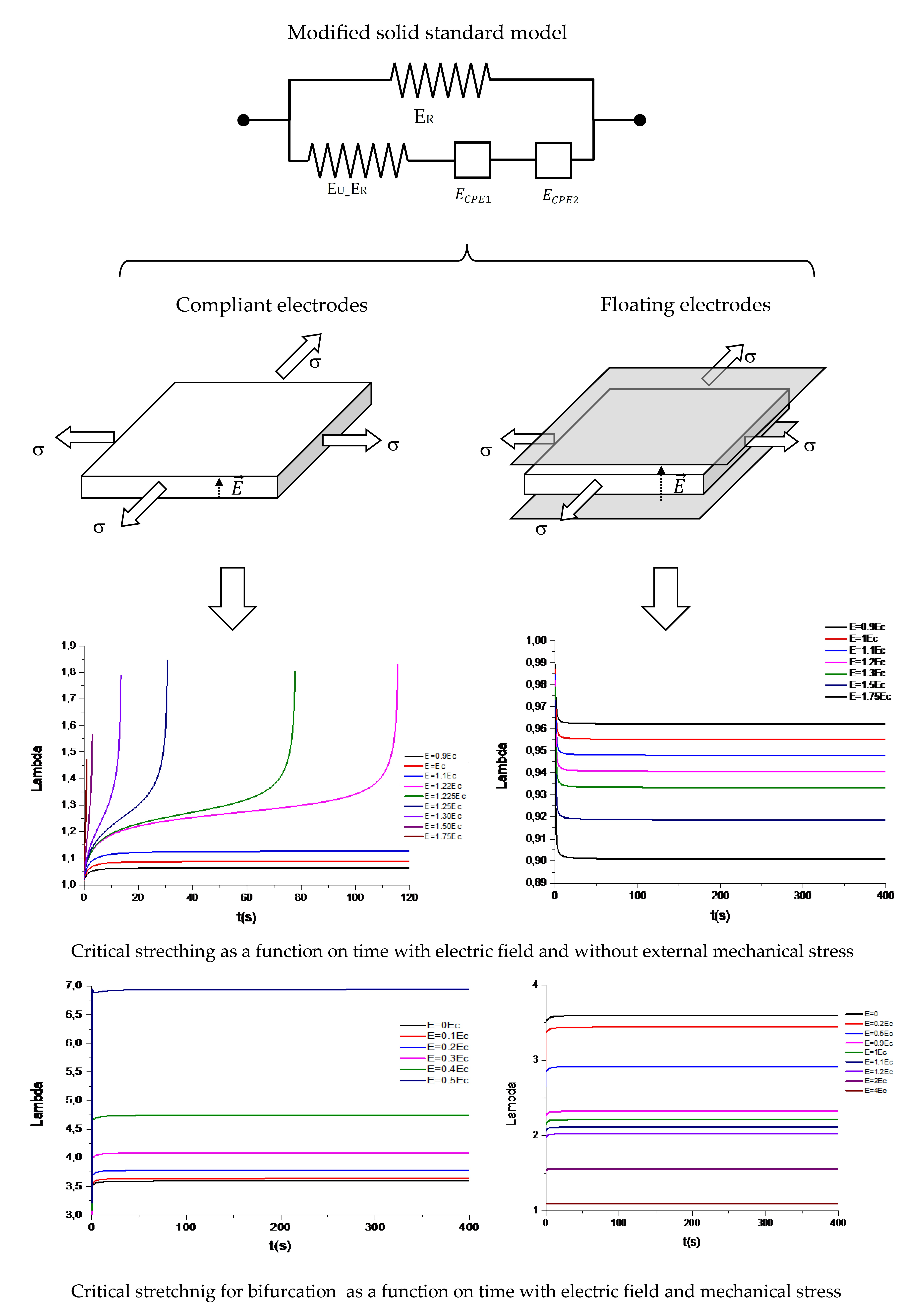
4] have recently proposed an approach to give an account of the dissipative viscoelastic behaviour of the dielectric elastomers based on the CIT. On this basis, they have constructed a theory that, as a particular case, includes the annihilation of the classical hessian determinant to determine the stability or instability conditions. The aforementioned theory requires new ingredients to give an account of the irreversible processes suffered by the material during the relaxation processes. Then, a set of internal variables are included as a part of the Helmholtz free energy density. Subsequently, a differential equation to represent the kinetics of the actual irreversible processes appears. This differential equation needs to be solved in conjunction with the constitutive stress–strain relations derived from the free energy density. Suo et al. rightly state that ‘there is considerable flexibility in choosing kinetic models to fulfil the thermodynamic inequality’, which, in fact, is derived as a consequence of the second law of thermodynamics. In any case, the choice should be experimentally consistent. On this basis, an order one kinetic has been chosen to illustrate the general approach. A first-order kinetic, which is represented by a first-order differential equation, is equivalent to considering a single relaxation time associated with the relaxation process. This relaxation time is related to the dashpot appearing in the classical solid standard model (Zener model). It should be stressed that two types of standard solid models are possible. One is a spring in parallel with a Maxwell element, that is, a spring with a dashpot in series (
Figure 1a), and it is used in this paper as the basis of the more complex models. The second one is a spring in series with a Kelvin–Voigt element, which is a spring in parallel with a dashpot (
Figure 1b), and it has been used by other authors [
2,
7]. The first model is related to the case of a strain input (stress relaxation experiment), whereas the second one corresponds to the case in which a stress input is used (creep experiment). The parameters of both models are obviously related [
15], and similar models have been proposed for the case of dielectric relaxation processes [
18].
In this respect, the simplest dielectric model corresponds to the results of the classical Debye theory of the dielectric relaxation based on the rotational Brownian motion [
25], which considers a single relaxation time. In fact, the Debye equivalent electric circuit includes two capacitors representing the passive elements for the storage of the electrical energy and a resistor to give an account of the dissipative process. The mechanical equivalent circuit in the electromechanical analogy is, of course, the above-mentioned Zener model consisting of two springs and a dashpot. However, the single relaxation time model initially proposed by Debye requires modification in order to fit the experimental results of the materials under study because of the actual presence of a distribution of relaxation times. A first alternative model was proposed by Cole and Cole [
26] after studying the dielectric properties of some alcohols, showing non-Debye behaviour. This model implies the substitution of the resistor in the electric circuit by a CPE, which is an empirical impedance function (see
Appendix A) and has a parabolic form in the time domain as can be found in the literature [
16,
18]. It is noticeable that the introduction of a CPE induces the appearance of a distribution of relaxation times. However, in the case of polymeric materials, the experimental data and the corresponding relaxation time spectra show a nonsymmetric shape. As a consequence, Havriliak and Negami (HN) [
27] have modified the Cole–Cole model (CC) [
26] to represent accurately the actual dielectric relaxation data of most of the polymers. The HN model predicts in fact a nonsymmetric relaxation time spectrum in agreement with the nonsymmetric shape of the experimental data and has been extensively used in practice. As an alternative to the HN equation, a biparabolic model has been proposed by Huet [
28,
29], which includes two CPEs. Each one of these CPE accounts for, respectively, the low- and high-frequency sides of the spectra. It should be noted that the parameters of the HN equation are closely related to those of the biparabolic equation [
18] (p. 205). The equivalent mechanical model is easy to obtain, taking into account that the permittivity is, in the electromechanical analogy, mechanical compliance and assuming that the corresponding mechanical counterpart is an electric modulus. It should be noted that in mechanical terms the adoption of a CPE is equivalent to assume, instead of a simple Newtonian behaviour, a non-Newtonian one for the mechanical dissipative element. On this basis, a modification of the kinetic model used in [
4] is pertinent.
3. Formal Analysis
The starting point to the formal analysis of the viscoelastic behaviour is the standard solid model proposed in [
4] (
Figure 1a), which is formed by a spring in parallel with a Maxwell element, that is, a spring in series with a dashpot. However, due to the fact that the viscoelastic primary data are obtained from uniaxial tensile modulus, the parameters of the standard solid model refer to the relaxed and unrelaxed tensile moduli and the corresponding tensile viscosity (respectively, E
R, E
U, and η
E).
The differential equation governing this model is given by
where
and
are, respectively, the stress and the strain,
is the characteristic relaxation time,
(
) is the viscosity coefficient associated with the dashpot, and
are, respectively, the relaxed and unrelaxed tensile modulus. In forming this differential equation (see Ref. [
15]), the following relation between the stress in the Maxwell element in parallel and the strain in the dashpot is used:
where a superscript dot indicates time derivative. Equation (2) corresponds to the classical Newtonian behaviour in the dashpot.
The stress response of the model given by Equation (1) in the time domain to a strain input given by
, where
is the unit Heaviside function (step function), is given by
This seems to be the type of response depicted in
Figure 2b of [
4].
Then, the corresponding relaxation modulus in the time domain is given by
and the dynamic modulus in the frequency domain is obtained from the Laplace transform of both sides of (4) and is defined by
where
,
, and
is the defined dynamic modulus.
This is the classical single relaxation time dynamic response in the frequency domain corresponding to the standard solid model.
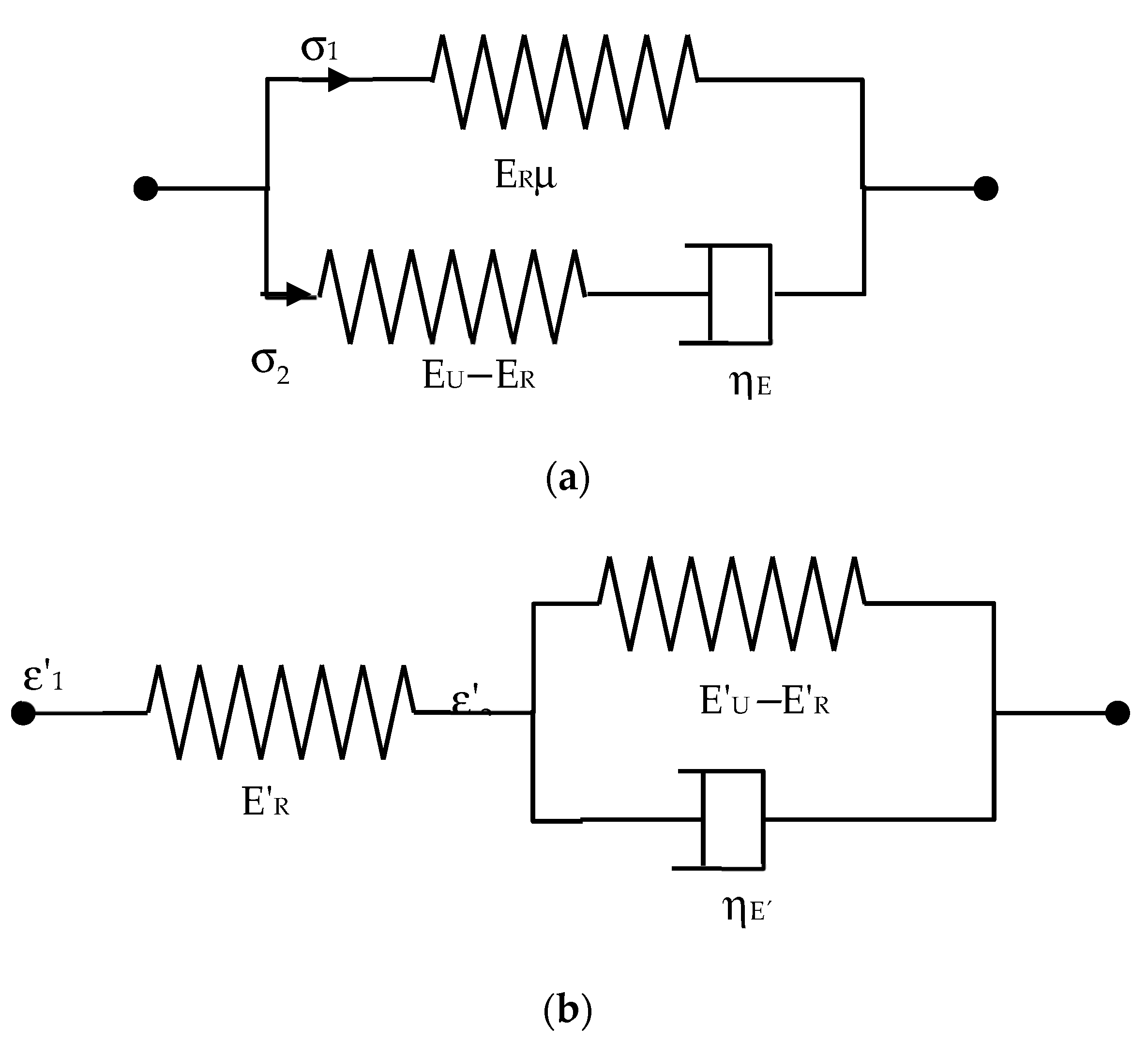
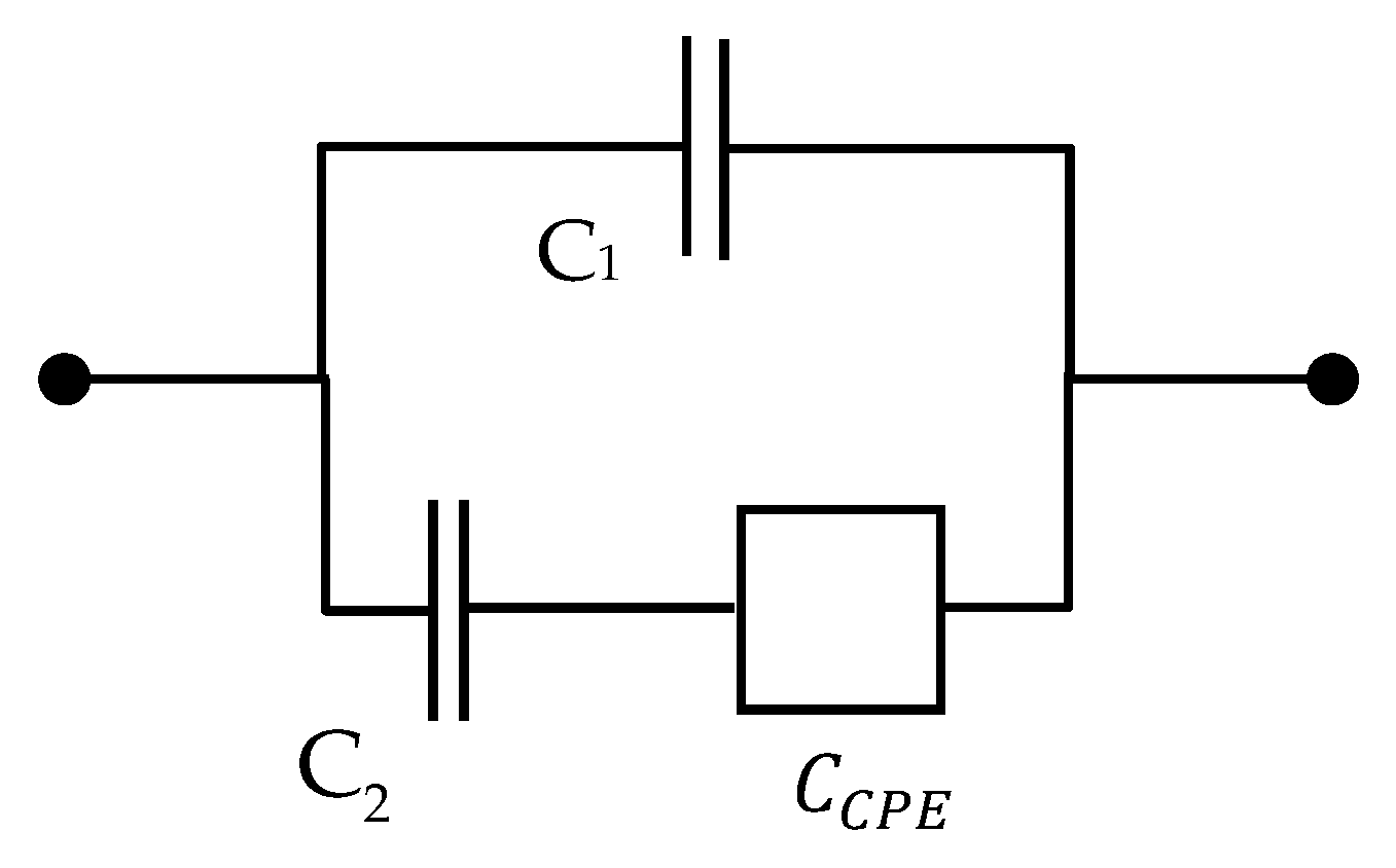
However, in order to give an account of the observed distribution of relaxation times experimentally observed, there are several possibilities, but in the present case, a slightly more sophisticated model is considered, as the one shown in
Figure 2, where a mechanical CPE instead of a dashpot is used. The empirical mechanical impedance of this CPE may be expressed in terms of the parameters shown in
Figure 2 as
where
.
Taking into account Equation (6), the total mechanical impedance of the scheme, represented in
Figure 2, may be found as the addition of the impedance of the upper branch of the scheme in that figure and the inverse of the addition of the inverses of the impedance of the two elements of the lower branch of the same figure.
Since represents in the time domain the first-order derivative with respect to the time, can be interpreted in the present context as a fractional derivative of order . The introduction of the constant is enough to create a distribution of relaxation times corresponding to the viscoelastic model given by Equation (7).
It can be shown that this result should be obtained by assuming a new relation between the stress and the rate of strain in the dashpot as follows:
where
and
are, respectively, the stress in the bottom branch of the scheme shown in
Figure 2, and the strain in the CPE of this Figure, and
is a pseudo-viscosity.
Equation (8) may be considered as corresponding to a ‘fractional dashpot’ where refer, respectively, to the ideal plasticity and the Newtonian liquid. In our case, being the obtained result in the time domain corresponds to the situation of nonexponential stress relaxation, as observed in the actual experiments.
Of course, more complex models different from that given by Equation (8) should be assumed as it will be shown later. Then, taking into account Equation (8), the differential Equation (1) is modified, and thereafter, the pertinent algebra can be reformulated according to (see
Appendix B)
where
, being
the pseudo-viscosity, and
denotes the fractional derivative of order
of a function
.
It is a well-known fact that there are several kinds of fractional derivatives [
22]. In this work, we have chosen the Caputo derivative because its properties make it possible to consider initial conditions in terms of the value of the function
as is required in our context. The intuitive meaning of Caputo derivative lies in the concept of fractional integral, termed Liouville fractional integral, which is defined by
where
is the Euler’s Gamma function. Then, the Caputo derivative is defined by
where
(being
the greatest integer less than or equal to
), and
denotes de
-th ordinary classical derivative of
. Intuitively, in order to obtain the Caputo fractional derivative of
of order
, first, it is necessary to differentiate
times the function
and then to integrate the exceeding part. This latter term, consisting of calculating an integral (thus involving the evaluation of the function
over its integration domain), allows the interpretation of the Caputo derivative as a ‘memory’ operator since it takes into account the physical ‘history’ described by the function
. In numerous physical contexts (see, for example, Refs. [
30,
31]), the Caputo derivative has demonstrated to successfully capture the ‘past history’ of the corresponding phenomena under study described via the function
. Furthermore, it is easy to check, by means of the application of integration by parts the formula to
, that the Caputo derivative becomes the ordinary derivative when
is a positive integer, thus retaining the physical meaning of the classical derivative.
In our case, we consider that
; thus, the Caputo derivative of this specific order is given by
Differential models in viscoelasticity including fractional derivatives were suggested by several authors [
32,
33,
34,
35,
36,
37] and used in connection with the viscoelastic or dielectric time-temperature superposition [
38].
It is noteworthy that the dielectric counterpart of the mechanical model (
Appendix A) consists of a capacitor with capacitance
in parallel with a series coupling of a capacitor with capacitance
and a CPE, as represented in
Figure 3.
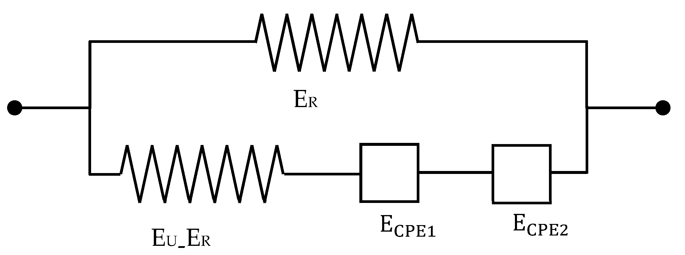
4. Generalisation for Non-Symmetric Relaxation Spectrum
As mentioned above, Equations (7) and (A5) predict a symmetric distribution of relaxation times [
18], which is unlikely for polymeric materials. For this reason, a biparabolic model with two constant phase elements is proposed to represent the dynamic shear viscoelastic data [
18]. The corresponding mechanical model is shown in
Figure 4.
In a similar way to how is conducted in Equation (6), one can write
for, respectively, the low- and high-frequency side of the spectrum. This explains why only two continuous phase elements at least are necessary.
Thus, after the pertinent calculations similar to those of
Appendix B, the dynamic tensile modulus can be expressed as
where
,
, and
is a parameter associated with the nonsymmetric shape of the spectrum [
39].
At this point, it is important to note that the viscoelastic parameters appearing in Equation (14) refer to the dynamic tensile modulus, whereas the elastic parameters that appear in the free energy density correspond to the shear modulus. In general, the relationship between the tensile and the shear viscoelastic moduli is given by
where
is the viscoelastic Poisson ratio. For incompressible materials, the Poisson ratio is commonly taken as
due to the incompressibility assumption. For this reason, in those that follow and in order to relate the dynamic viscoelastic tensile modulus to the dynamic shear modulus, the following equation is taken:
In these conditions, in those that follow, a similar expression to that of Equation (14) is taken for the shear modulus, that is,
The use of the shear modulus is justified because from the Hooke’s law and the relation between the stretching and the deformation for relatively small deformations, the classical result is obtained, where N is the number of chains of the network, is the Boltzmann constant and T the absolute temperature. As will be seen later (see Equations (31) and (32)), the shear modulus of the material is closely related to the parameters and appearing in Equation (18a,b) for the free energy density.
A similar model to the one presented in Equation (17) should be assumed for the dielectric permittivity of the elastomer by taking into account that the permittivity is a compliance function. However, as mentioned above, the dielectric relaxation process takes place very quickly in comparison with the viscoelastic one and, in these conditions, the dielectric relaxation process is in equilibrium, that is, the material is fully dielectrically relaxed when the viscoelastic process starts. On the other hand, it is assumed that possible conductive relaxation processes in the elastomer, which currently are proportional to , are significantly active at frequencies considerably lower than the viscoelastic relaxation processes, and, for this reason, no overlapping between these two processes is expected. In Equation (17), and are, respectively, the fractional-order of the derivative, and the two relaxation times.
In order to obtain a better fit of the experimental results, a modified Mooney–Rivlin model has been chosen for the free energy density instead of the neo-Hookean one. Accordingly, the free energy density for the case in which viscoelastic effects are present may be written as
In the present approach, it is assumed that the permittivity
does not depend on the strain. As it has been discussed in another study [
40], the polarity of the acrylic VHB 4910 elastomer corresponds to a type C polymer (in the classical Stockmayer´s terminology [
41]), in which the dipoles causing the main dielectric activity are in the lateral chains and, according to it, they are separated from the backbone by flexible segments, and therefore, its permittivity should be scarcely affected by stretching.
Equation (18a) is a generalisation of Equation (17) of the Ref. [
4] useful for our purposes. In this equation,
and
with
are the relaxed and unrelaxed shear moduli for the two branches of
Figure 4. The first two terms on the right-hand side represent the elastic energy of the spring at the top of the scheme given in
Figure 4. The third and fourth terms in this Figure correspond to the bottom branch of the before mentioned scheme. Moreover,
are the stretches due to the two dashpots. Two subindexes are used to describe the stretching in these two dashpots: the first one refers to each one of the two in-plane stretches, whereas the second refers to the two CPE existing in the model. The last term represents the electrostatic energy of the material, with
being the nominal dielectric displacement. The relationship between the nominal dielectric displacement and the nominal electric field is given by
, where
is the dielectric permittivity, and
is the nominal electric field. In the forthcoming calculations, it is assumed that the permittivity is not dependent on the stretches. Of course, many other empirical or semiempirical models should be checked, but for the present purposes, the chosen approach suffices.
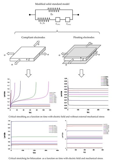
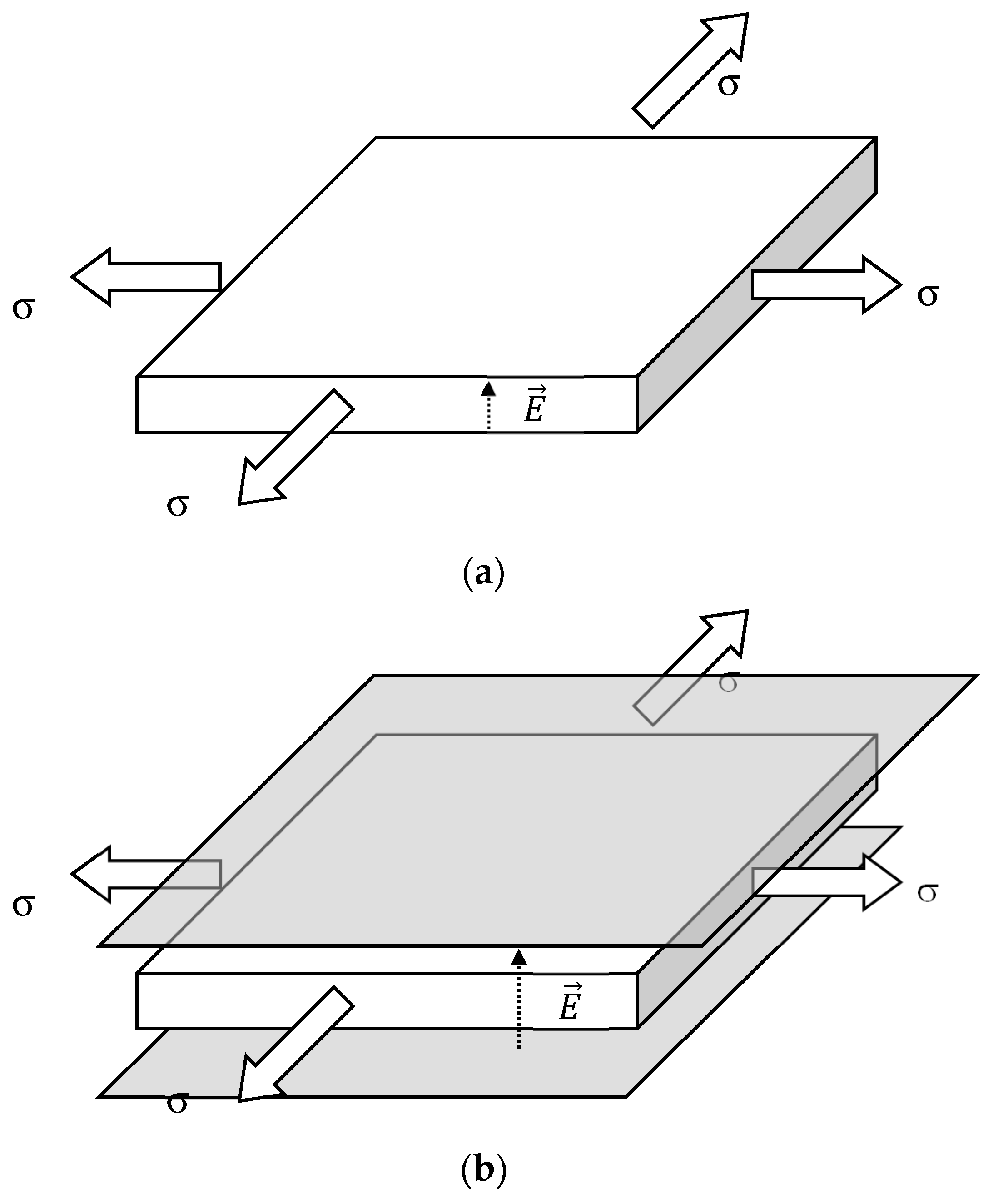
It is noted that Equation (18a) is valid for the case of compliant electrodes (
Figure 5a), that is, for the case in which the electrodes are deposited on the two faces of the sample, by ion sputtering, for example. However, in some circumstances, for example, nematic liquid crystal elastomers [
42], the constrained geometry is avoided in order to eliminate anchoring effects in the boundaries of the sample. To accomplish this purpose, a gap between the sample and the electrodes is adjusted using adequate spacers in such a way that the distance between the electrodes is maintained systematically larger than the thickness of the sample (
Figure 5b). The gap should be large enough to prevent pull-in phenomena.
In that case, the Maxwell stress tensor between the sample slab and the electrodes should be taken into account, and the free energy density, taking into account the viscoelasticity, is now given by
where
is the permittivity of the fluid where the sample is floating, which usually is the air.
Let us assume that geometry under consideration refers to a squared plate of electroviscoelastic material subjected to two pairs of forces or deformations in the principal directions. An electric field is applied perpendicular to the plate.
For equibiaxial stretches and in order to simplify calculations, it is assumed that
Then, the following equations for the stresses and the electric field together with two kinetic equations are found (see
Appendix C).
for Equation (17), and
for Equation (18b).
Note that the equations for (20a) (3rd equation) and (20b) (3rd equation) are the relation between the nominal electric field and the nominal displacement, to be used later.
Then, according to the methodology outlined in
Appendix C and, after the pertinent algebra, one obtains for the kinetic restriction equations,
where the initial conditions are
, and
.
It should be noted that there are many possibilities with respect to the choosing of the kinetic models to fulfil the thermodynamic requirements expressed by Equation (A14) in
Appendix C. They are closely dependent on the properties of the electroelastic material under consideration.
7. Numerical Calculations
As the differential fractional algebraic equations (DFAE) given by (21a,b) do not have a closed solution, we approximate its solution by using a numerical method combining the fractional forward Euler method, for fractional differential equations applied to Equation (21a,b), and an iterative method to find the roots of the algebraic restriction given by Equation (30a,b). To explain the used methodology, an equation for a generic stretch
is considered. In this way, given a fractional initial value problem,
By Theorem 3.1 of the Ref. [
52], we can obtain the Volterra integral equation associated with the problem above, that is,
To obtain an approximate solution, first, we consider a discretisation of the fractional integral,
, based on an equally spaced mesh for the time variable
with
nodes defined in the interval
and
The numerical approximation of the fractional integral of
in
is given by
Observe that, in the first step, we have split the integral on the time interval
, into
integrals on the time intervals
, in the second step, we have approximated the function
over the whole interval
just by
, and, finally in the last step, the remaining integral has been computed. With this approximation, we obtain the fractional forward Euler method, which is an extension of the classical Euler method as follows:
According to our initial value problem, the fractional Euler method is given by
where
, and
and
are the approximations of
and
in
Notice that in Equation (37),
is obtained in terms of approximations constructed in previous nodes. The value of
is selected small enough to obtain a converged solution in each one of the models analysed.
These equations are valid for each one of the two appearing in Equation (21a,b), and in this sense, the resulting equations are easily obtained from the former ones.
Once
is obtained, the value of
is computed by finding the root of the equation for compliant electrodes (or their counterpart equation for floating electrodes),
which is closer to
. This root is computed numerically by using a combination of bisection, secant, and inverse quadratic interpolation methods [
53].
This strategy is easily generalised when, as in our case, two parameters, , appear in the restriction Equation (30a,b).
The following parameter is used in the calculations,
, being
the permittivity of the evacuated space. The critical electric field is given by
(see
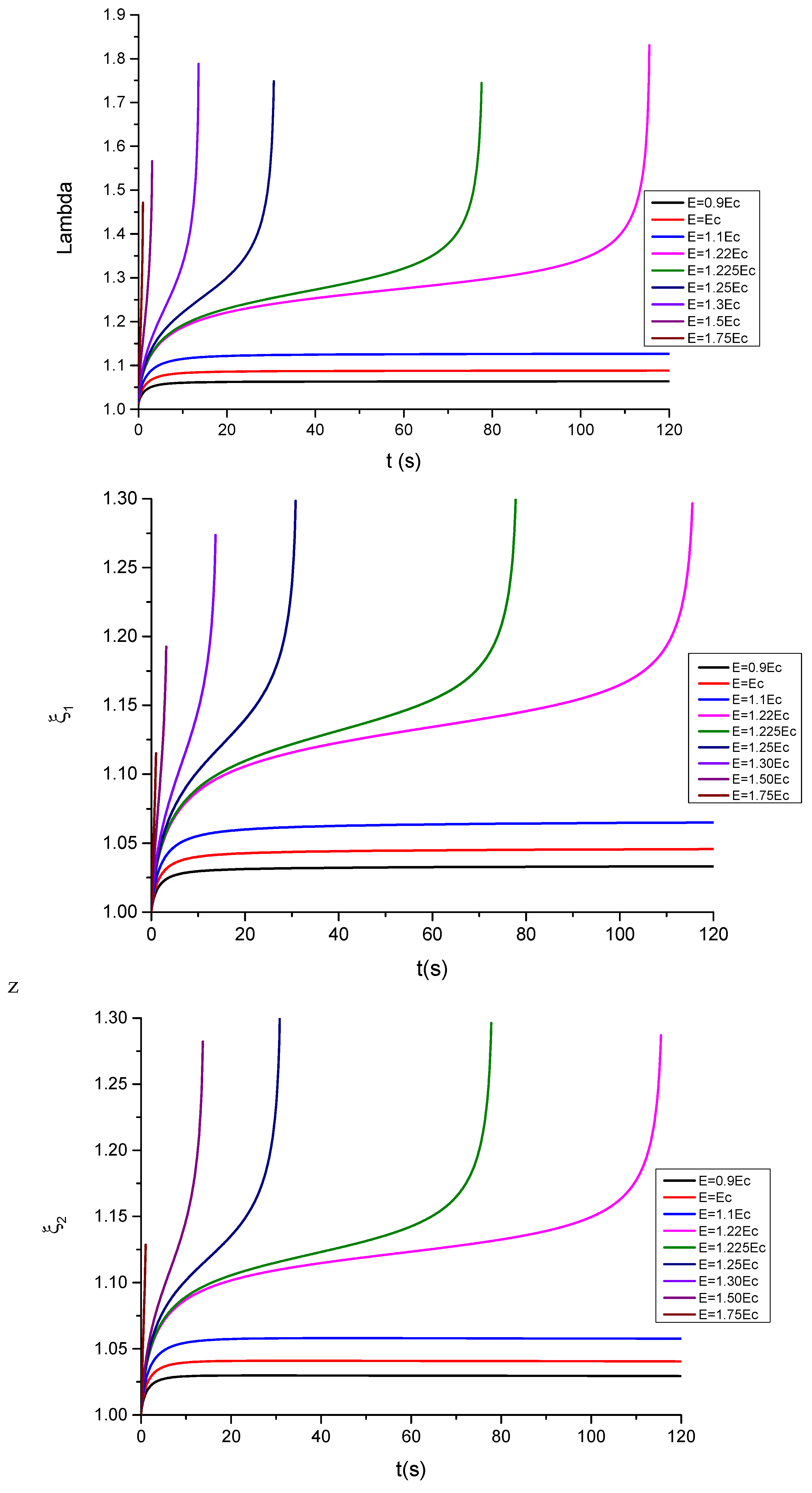
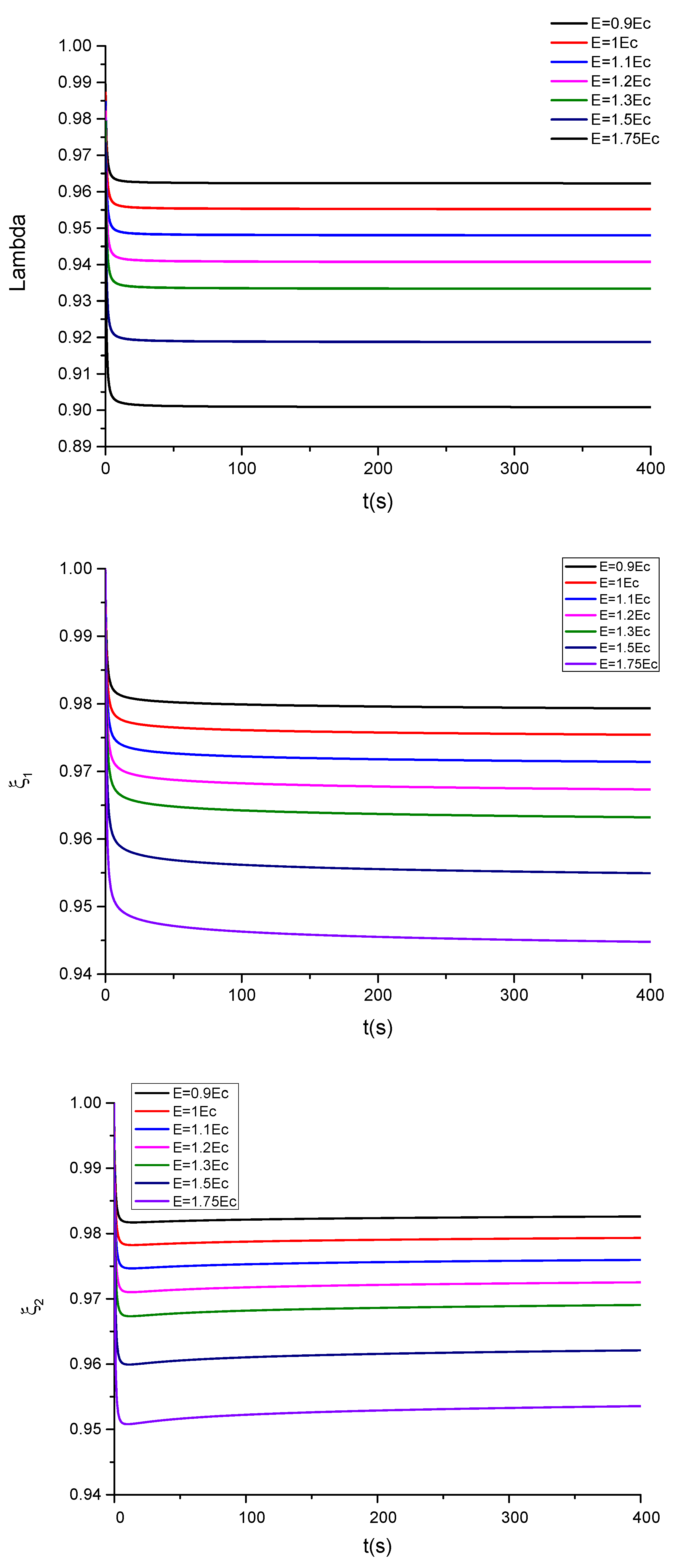
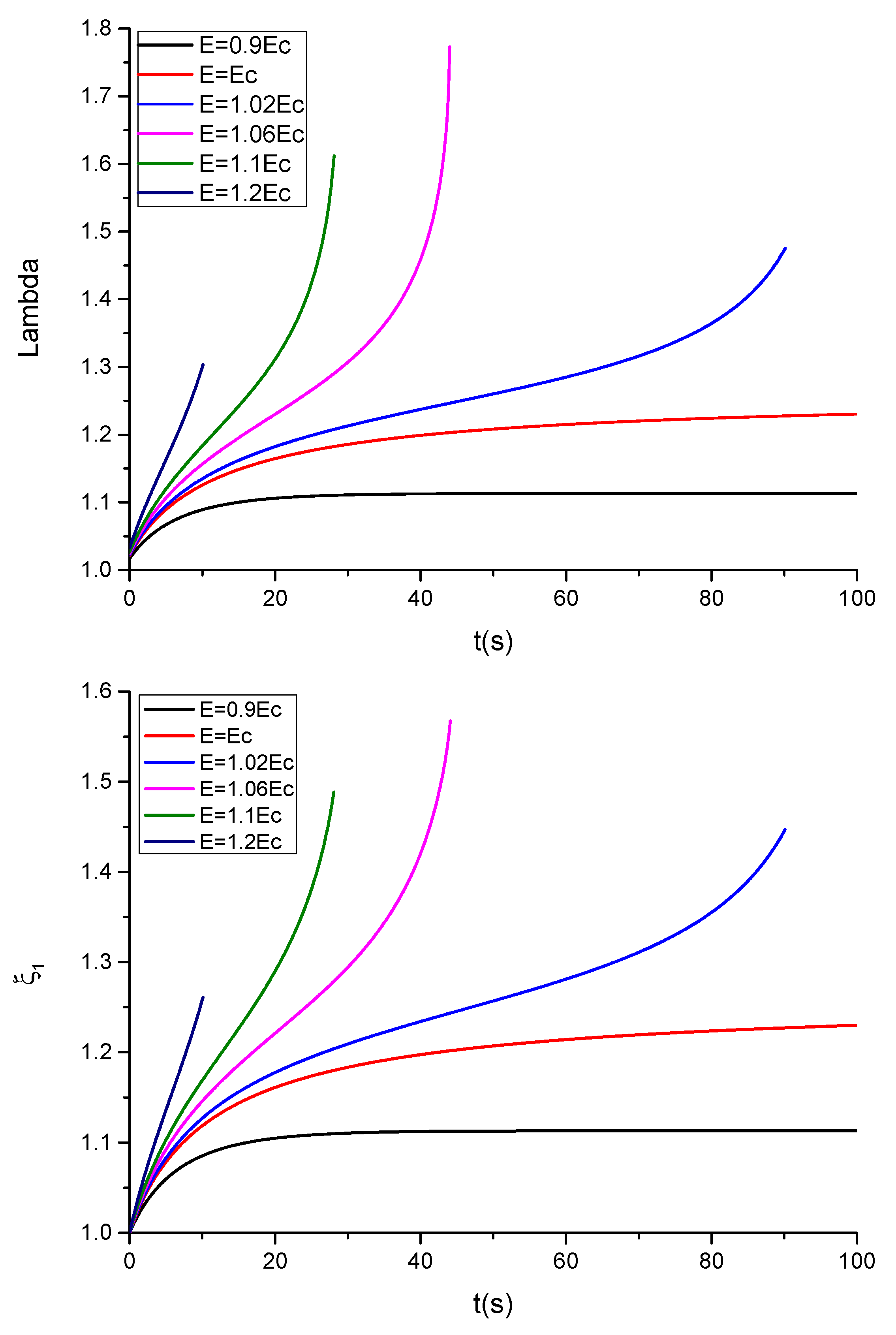
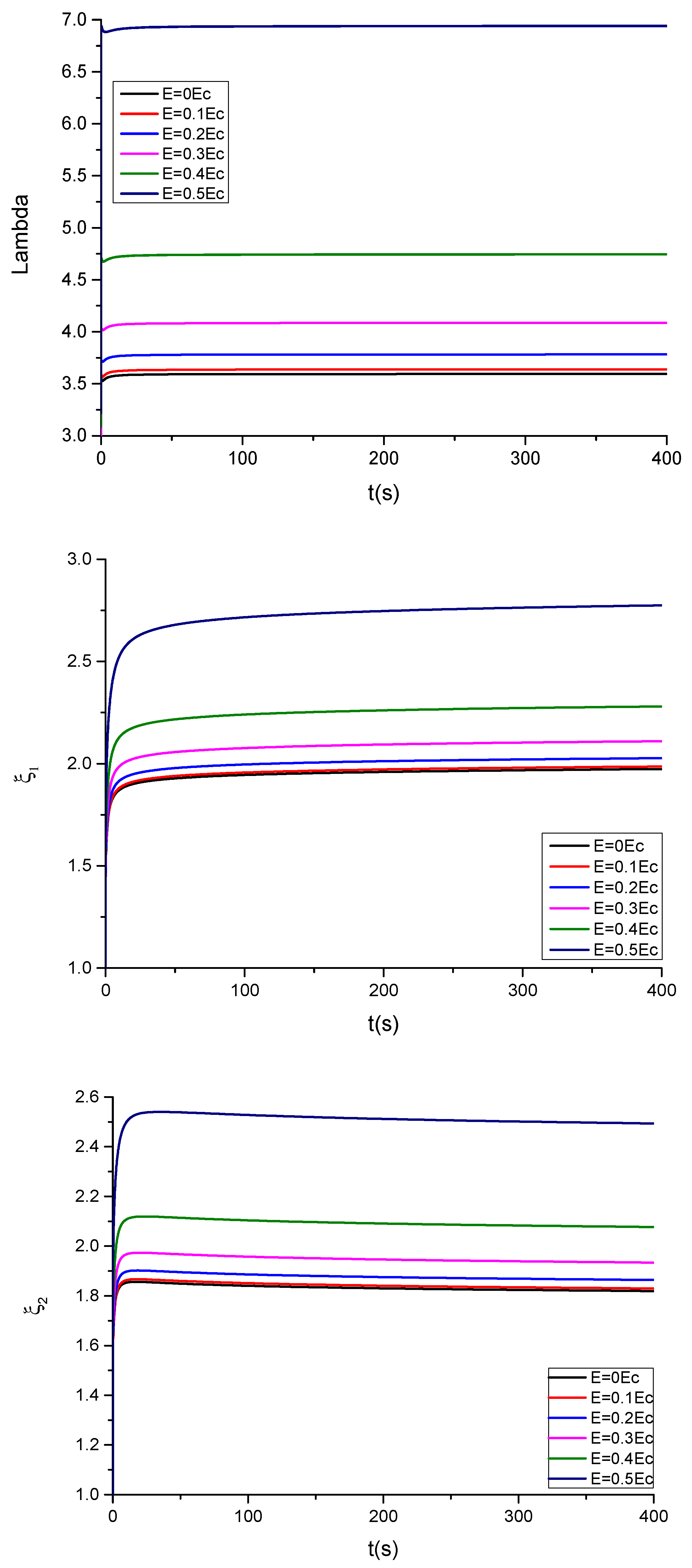
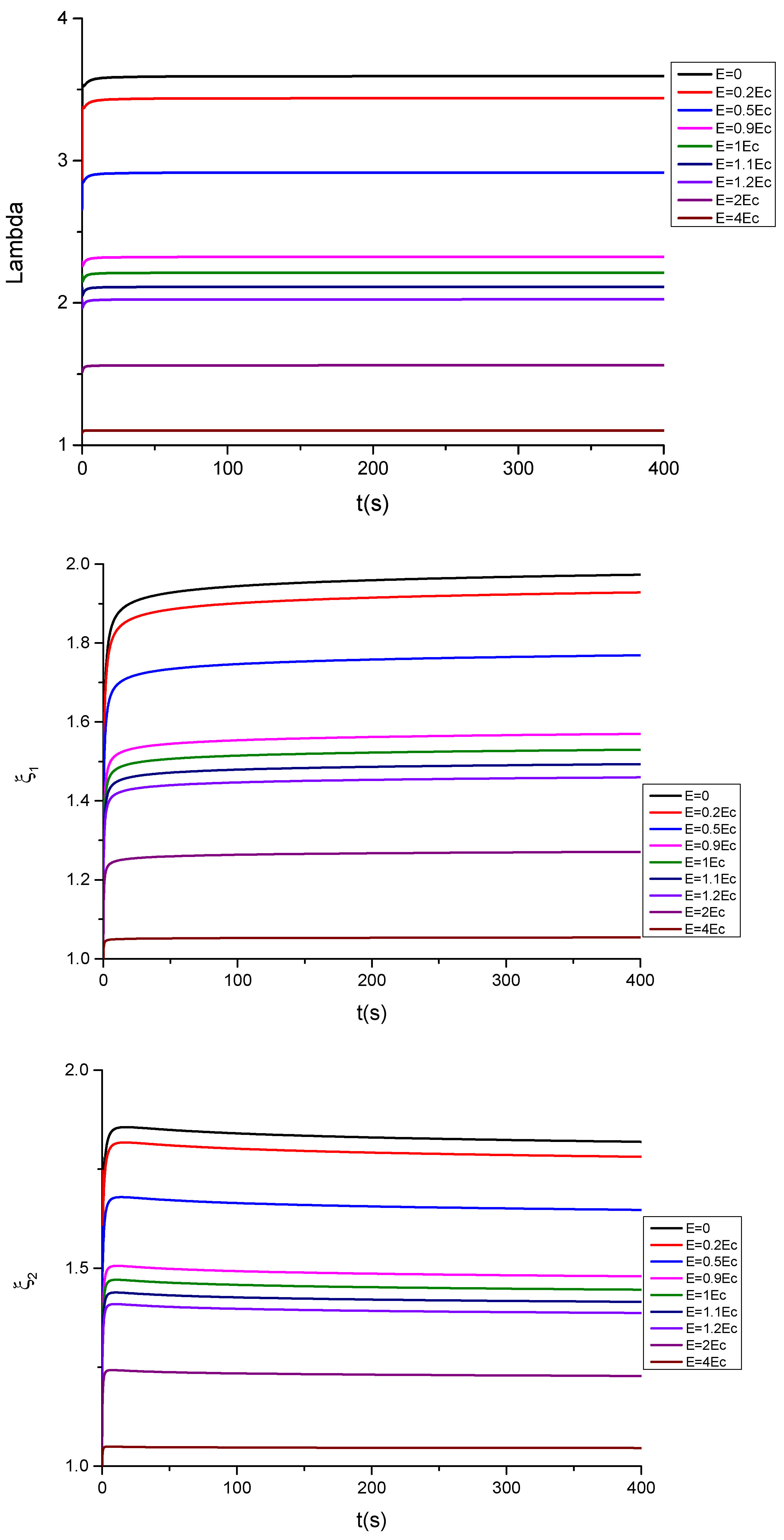
Appendix E). The corresponding results for the time evolution of
are shown in
Figure 6 and
Figure 7 for, respectively, compliant and floating electrodes and several electric fields.
The calculations have also been carried out for the case of a neo-Hookean model with a viscoelastic response in compliant mode governed by a single relation time (
), together with the following parameters:
as in the Equation (27) and
as indicated in
Appendix E and in agreement with Ref. [
44]. The corresponding equations are
with the corresponding kinetic equation given by
For purpose of comparison, the results obtained by Suo et al. for a single relaxation time have been recovered by using our calculation program and taking into account the following parameters taken from Ref. [
4]
, together with a value of
for the relative permittivity, as reported by Wissler and Mazza in Ref. [
16]. The agreement is excellent.
8. Stability and Bifurcation Analysis
In the linear theory of elasticity, solutions of traction boundary problems are unique, and the stress fields are also unique. This is a consequence of the linearity of the constitutive equations relating stress and strain. However, under finite deformations, the stress–strain relationships for rubbers are nonlinear, and unlike the linear theory, the uniqueness of the solutions is, a priori, not warranted. Concomitantly, the appearance of instabilities and possible bifurcation phenomena are expected. For this reason, stability analysis in order to check the possibility of the appearance of bifurcations is pertinent because nonlinear elasticity is exhibited by these electroelastic materials.
An analysis of the instability and possible bifurcation phenomena requires using Equation (18a) as starting point because in the case of the neo-Hookean model no instability and subsequent bifurcation, as expected, are predicted. The classical procedure outlined in [
54,
55] and based on the Hessian approach is followed here. Let us consider, as above, a slab whose thickness in the third direction is small, in comparison with the lateral dimensions subjected to two pairs of dead loads in these two directions. Moreover, a homogeneous electric field is applied in the third direction. Since the deformation and the field are basically homogeneous, the field equations are automatically fulfilled. For the case of equal dead loads on the four lateral surfaces, one has for each of Equation (18a)
After the pertinent algebraic calculations, the subsequent equation which can be factorised to give a symmetric solution defined by
that represents the bisector of the first quadrant in a
plot. Moreover, a nonsymmetric solution is found, which intersects with the symmetric solution after taking into account (19) for the values of
solving the following equations for, respectively, compliant and floating electrodes
The time-dependent parameters
at which the bifurcation occurs are obtained by solving Equation (43a,b), together with Equation (21b). The parameters for the Equation (43a,b) used in the corresponding numerical calculations are the same as the used in the previous calculations.
Figure 9 and
Figure 10, respectively, show the effect of the electric field on the time evolution of the bifurcation stretch
and
for compliant and floating electrodes because we are dealing with a time-dependent bifurcation. Of course, other bifurcation modes and more complex bifurcation maps should be obtained by using, for example, incremental methods (see, for example, Ref. [
56]), but for the present purposes, the approach used here is sufficient.
9. Discussion
The plot of the stretching
and of the parameters
of the dielectric elastomer under study for several applied electric fields in the compliant configuration is, respectively, shown in
Figure 6 and
Figure 7. In the case of compliant electrodes (
Figure 6), starting from t = 0, the material relaxes with time, and subsequently, the stretch increases. For
, the observed parameters tend to a new equilibrium state, but for
, the elastomer becomes unstable at progressively higher electric fields. These results are in qualitative agreement with those observed in [
4]. However, as can be seen in
Figure 7, in the case of floating electrodes, the values of
are lower than the unity decreasing with the time until an equilibrium value. This is due to the fact that the material sample is in compression under the effect of progressively higher electric fields.
In the case of a neo-Hookean material governed by a single relaxation time corresponding to
Figure 8, the instability appears at lower times, as previously observed [
4]. This fact suggests that the use of a more realistic model than the Mooney–Rivlin model is a more realistic strategy to achieve valuable results in the study of these materials.
The bifurcation analysis, which is shown in
Figure 9 and
Figure 10, indicates that the values of
at the bifurcation increase with the time for the case of compliant, as well as for the floating electrodes. It should be noted that for
and in absence of electric field, a value of
is obtained with
from the following bifurcation equation:
in agreement with the classical results. However, this value increases (diminishes) with the electric field for the case of compliant (floating) electrodes, in qualitative agreement with the results obtained in Ref. [
54].
10. Conclusions
In this paper, as usual, an empirical model for the free energy density for a visco-hyperelastic material, VHB 4910, has been used as an example. In the present approach, no modelling is carried out on the possible electrical relaxation or conduction processes, because, as mentioned in the Introduction Section, when the viscoelastic relaxation processes take place, their electrical counterparts have occurred several decades before. Moreover, the treatment of the viscoelastic effects on the response of electroelastic materials, as outlined by Zhao and Suo [
54], is modified in order to consider (a) the Mooney–Rivlin model instead of the neo-Hookean one, (b) a distribution of relaxation times instead of a single relaxation time, and (c) the asymmetric character [
27] of the observed viscoelastic relaxations instead of a symmetric (CC) arc [
26]. For this purpose, fractional derivatives are used in order to construct the respective constitutive equations, as explained in
Section 3. The results obtained in the present paper suggest that the use of fractional derivatives for modelling the viscoelastic behaviour of electroelastic materials can give an account of the distribution of dielectric relaxation times. This seems to be a more realistic approach than those previously used to calculate the time evolution of the stretch
and the viscoelastic parameters
of these materials on the basis of a single relaxation time. Moreover, from the experimental point of view, the cases of compliant as well as floating electrodes are analysed. Both cases give very different results.
In order to compare our results with the former studies, the calculations are also carried out for the case of a neo-Hookean model with a viscoelastic model governed by a single relaxation time taking into account the parameters as in [
4], and the agreement is very good.
On the other hand, the classical bifurcation analysis carried out for compliant as well as floating samples show results that are in agreement with those previously obtained for electroelastic, nonviscoelastic materials (Ref. [
54]). It is to be stressed that the results obtained should potentially be useful in the design of electroelastic sensors and transducers as well as biomedical applications [
57,
58], prostheses, and robots, for example, in the case of cylindrical geometry for aortic prosthesis [
59]. This is one of the main highlights of the present study, that is, to prevent the appearance of unexpected anomalous electroelastic responses.


 ,
, 


