
Construction of a TTT-η Diagram of High-Refractive Polyurethane Based on Curing Kinetics


Abstract
:
1. Introduction
2. Materials and Methods
2.1. Chemicals
2.2. Sample Preparation
2.3. Characterization
2.3.1. Differential Scanning Calorimetry (DSC)
2.3.2. Rheological Measurements
3. Results and Discussion
3.1. Construction of TTT Diagram
3.1.1. Determination of Tg0 and Tg∞
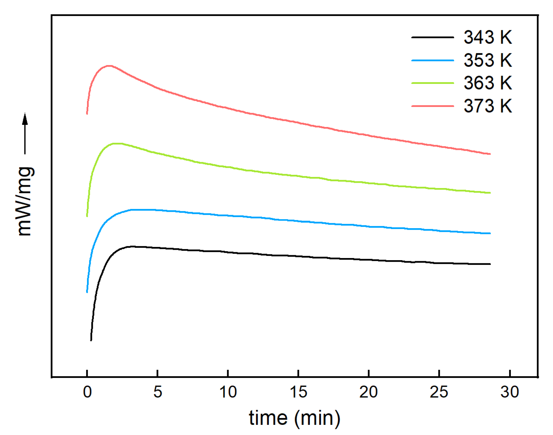
3.1.2. Determination of Iso–Curing Lines
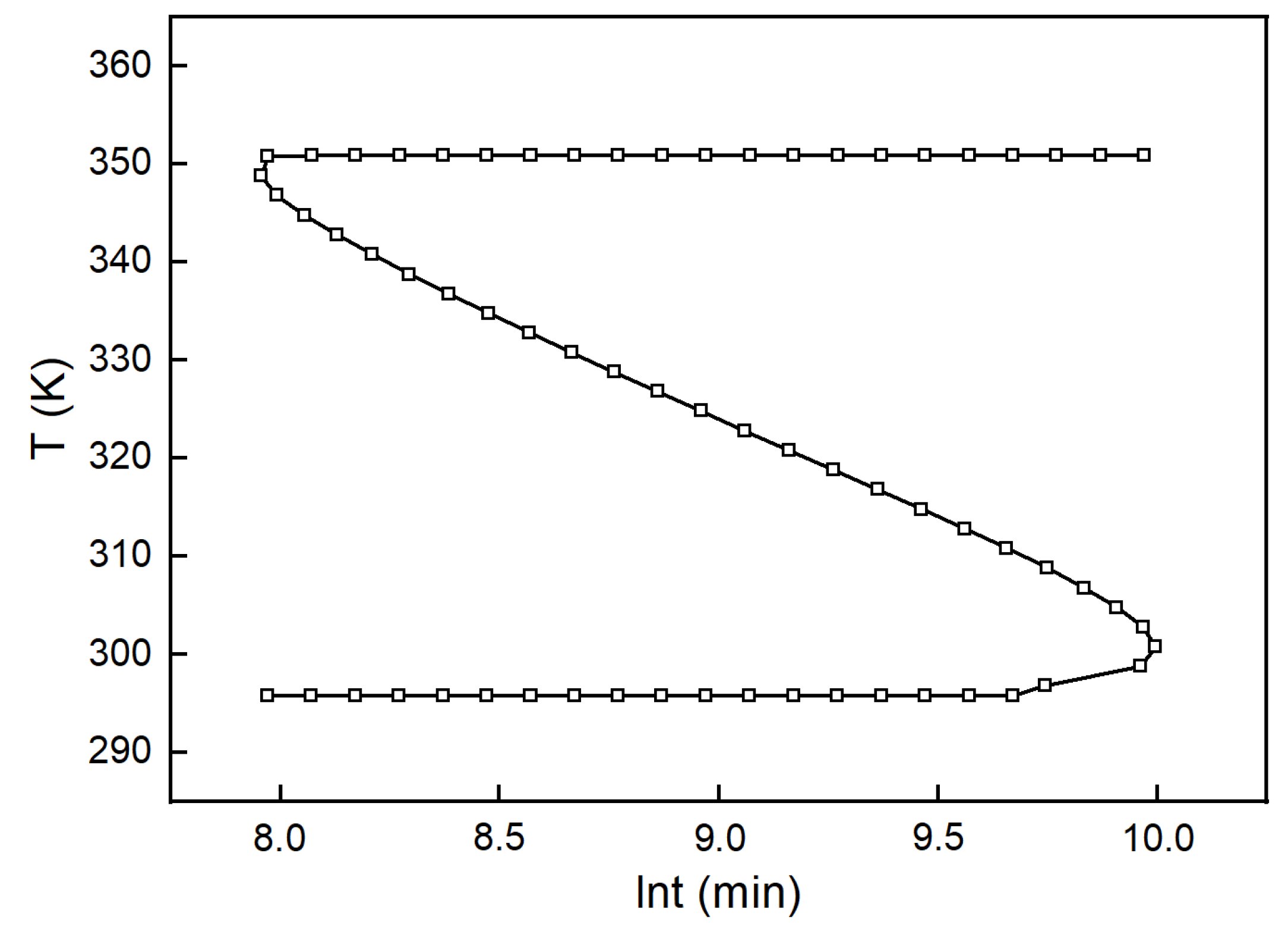
3.1.3. Determination of Glass Transition Curve
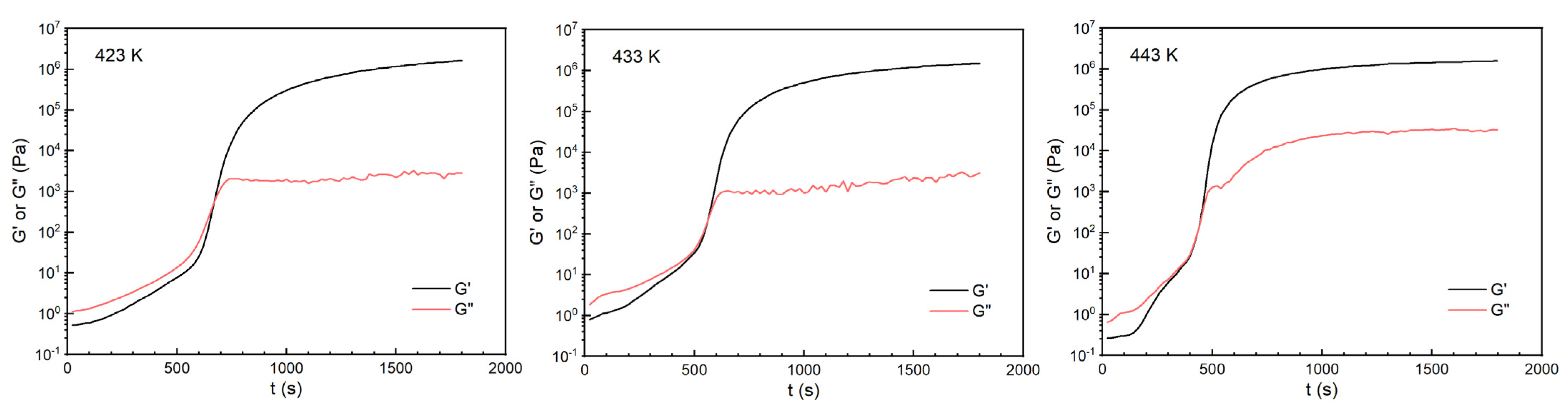
3.1.4. Determination of Gelation Curve
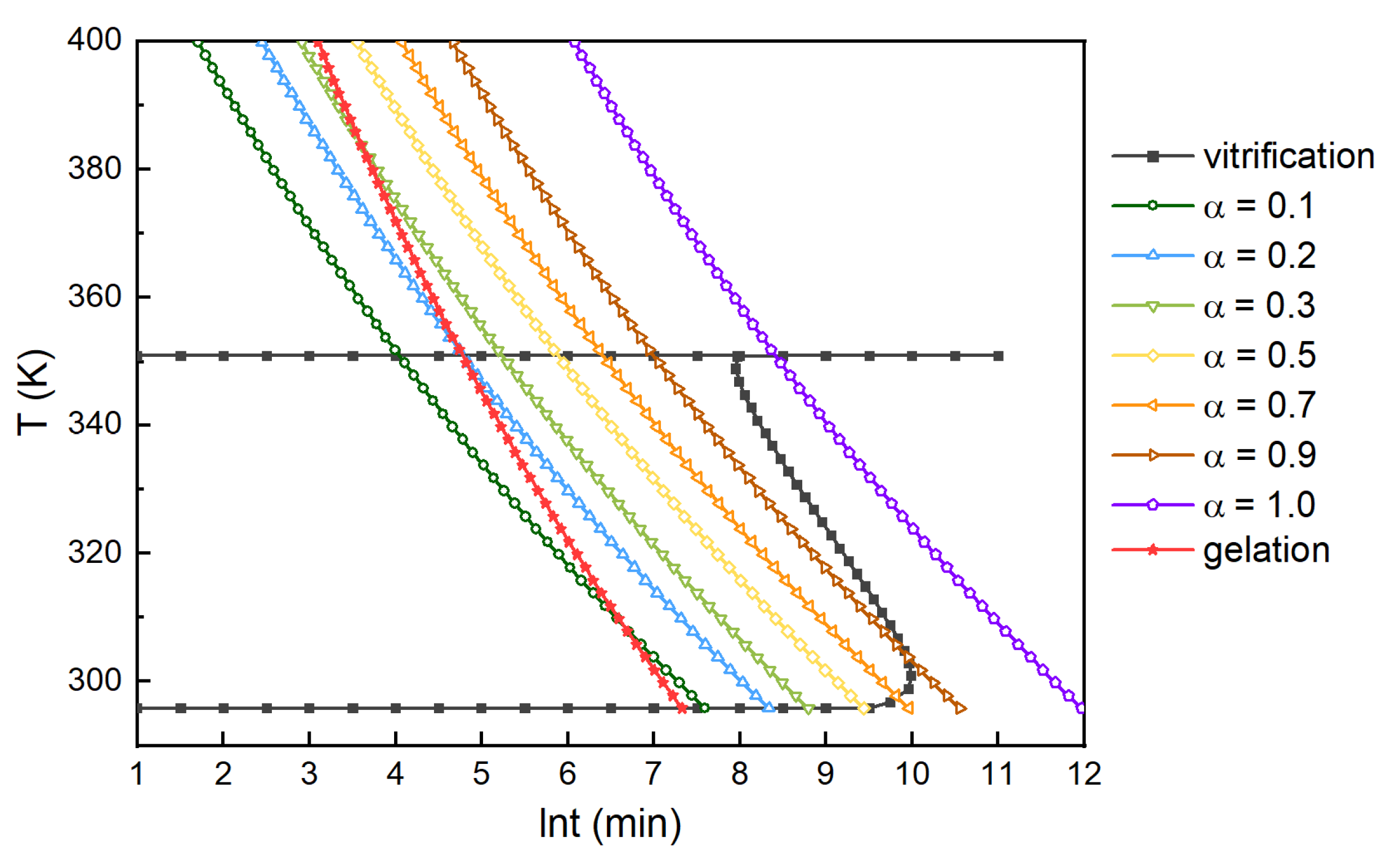
3.1.5. Construction of TTT Diagram
3.2. Construction of TTT-η Diagram
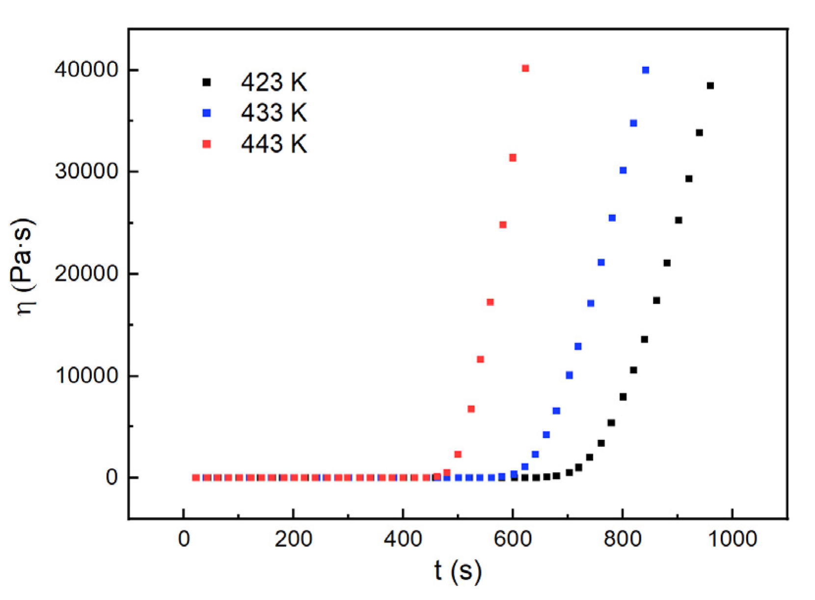
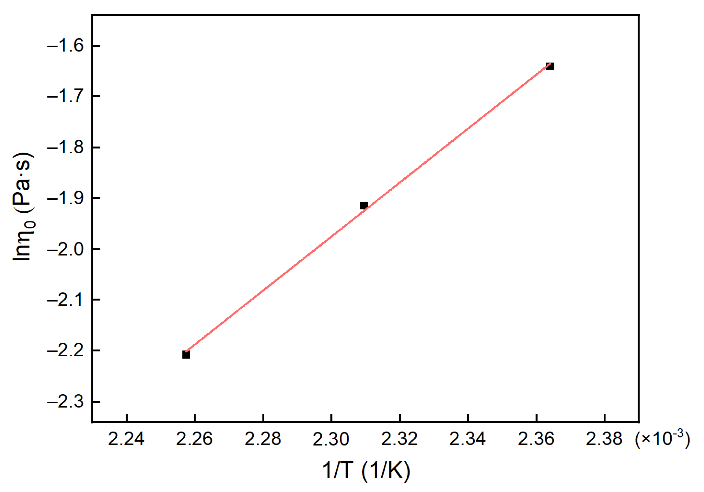
3.2.1. Fitting of the Initial Viscosity η0
3.2.2. Fitting for the Reaction Rate Constant K and the Pre-Exponential Factor A0
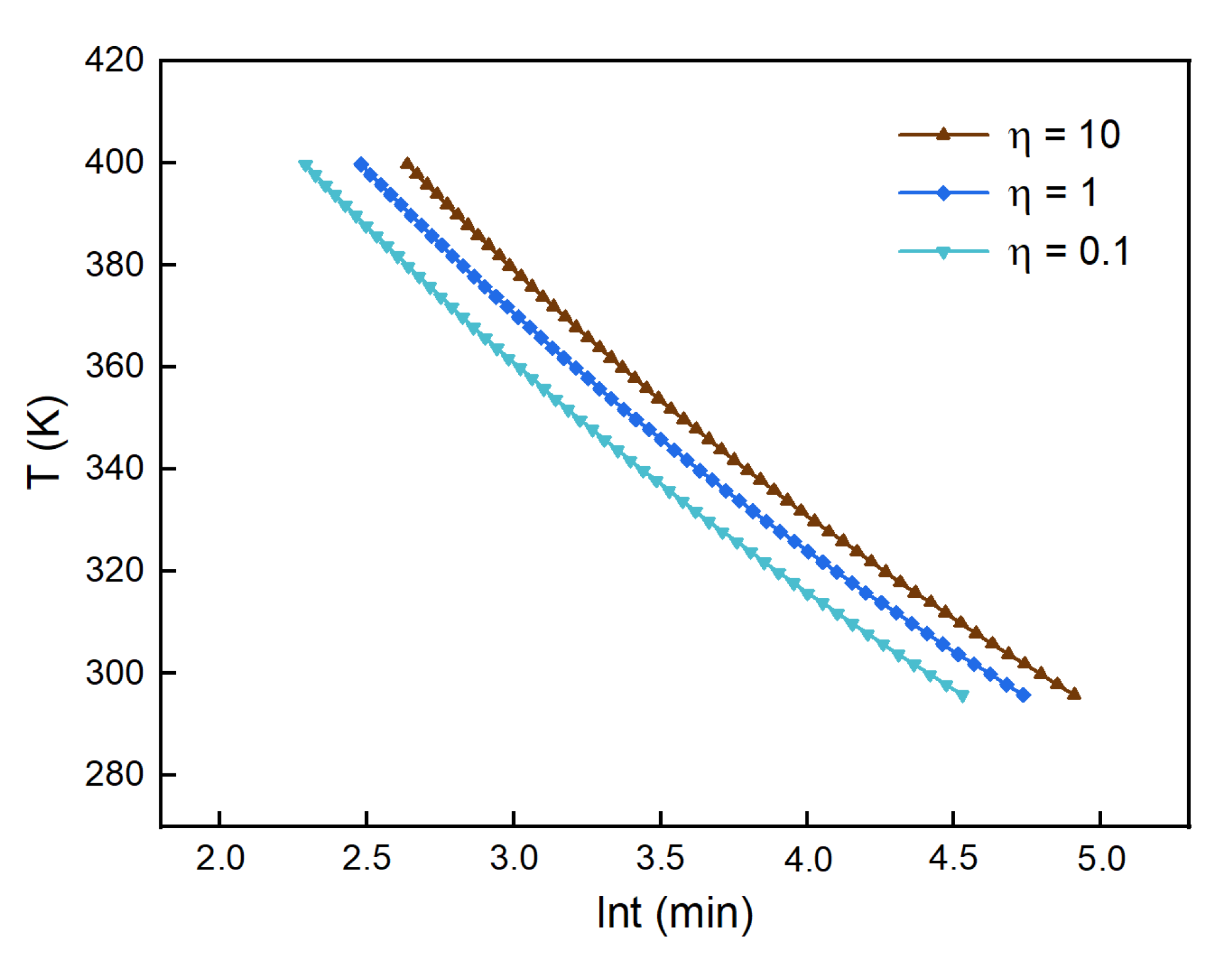
3.2.3. Construction and Verification of Rheological Model
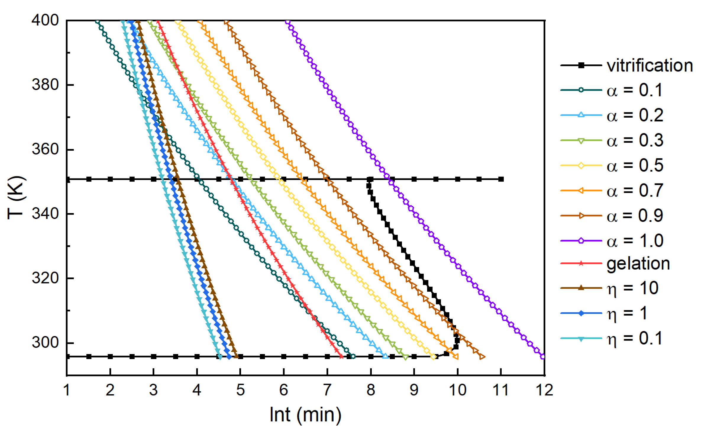
3.2.4. TTT-η diagram of H6XDI/BES System
4. Conclusions
Author Contributions
Funding
Institutional Review Board Statement
Informed Consent Statement
Data Availability Statement
Conflicts of Interest
References
- Zhang, M.; An, X.F.; Tang, B.M.; Yi, X.S. Cure kinetics and TTT-diagram of a bicomponent high performance epoxy resin for advanced composites. Acta Mater. Compos. Sin. 2006, 23, 17–25. (In Chinese) [Google Scholar]
- Zhang, X.F.; Yu, J.G.; Wu, Y.Q.Q.G.; Yi, X.S. Curing Kinetics and Isothermal Transformation (TTT) Diagram of epoxy resin using rosin–based acid anhydride as curing agent. Acta Polym. Sin. 2017, 3, 542–548. (In Chinese) [Google Scholar]
- Zhang, C.Q.; Chen, W.; Guan, Z.D.; Ye, H.J.; Zeng, L.S. Cure kinetics and TTT-diagram of the BA9913 resin. Fiber Reinf. Plast./Compos. 2017, 2, 48–53. (In Chinese) [Google Scholar]
- Teil, H.; Page, S.A.; Michaud, V.; Månson, J.A.E. TTT-cure diagram of an anhydride–cured epoxy system including gelation, vitrification, curing kinetics model, and monitoring of the glass transition temperature. J. Appl. Polym. Sci. 2004, 93, 1774–1787. [Google Scholar] [CrossRef]
- Restrepo–Zapata, N.C.; Osswald, T.A.; Hernández–Ortiz, J.P. Method for time–temperature–transformation diagrams using DSC data: Linseed aliphatic epoxy resin. J. Appl. Polym. Sci. 2014, 131, 40566. [Google Scholar] [CrossRef]
- Li, C.X.; Dai, Y.T.; Hu, X.P.; Zhang, H.; Zhou, L.P.; Liu, Z.H. Curing kinetics of TiB2/epoxy resin E–44 system studied by non-isothermal DSC. Resin 2011, 26, 6–10. (In Chinese) [Google Scholar]
- Khoun, L.; Centea, T.; Hubert, P. Characterization Methodology of thermoset resins for the processing of composite materials –case study: CYCOM 890RTM epoxy resin. J. Compos. Mater. 2010, 44, 1397–1415. [Google Scholar] [CrossRef]
- Kamal, M.R.; Sourour, S. Kinetics and thermal characterization of thermoset cure. Polym. Eng. Sci. 1973, 13, 59–64. [Google Scholar] [CrossRef]
- Kratz, J.; Hsiao, K.; Fernlund, G.; Hubert, P. Thermal models for MTM45–1 and Cycom 5320 out–of–autoclave prepreg resins. J. Compos. Mater. 2012, 47, 341–352. [Google Scholar] [CrossRef]
- Hickey, C.M.D.; Bickerton, S. Cure kinetics and rheology characterisation and modelling of ambient temperature curing epoxy resins for resin infusion/VARTM and wet layup applications. J. Mater. Sci. 2013, 48, 690–701. [Google Scholar] [CrossRef]
- Henrik, S. From the Kissinger equation to model–free kinetics: Reaction kinetics of thermally initiated solid–state reactions. ChemTexts 2018, 4, 9. [Google Scholar]
- Li, N.; Zhang, L.; Luo, X.; Wang, L.P.; Zhang, M. Study on Kinetics of Epoxy Resin Cured by Polyamides. Mater. Rev. 2015, 29, 565–567. (In Chinese) [Google Scholar]
- Nakka, J.S.; Jansen, K.M.B.; Ernst, L.J.; Jager, W.F. Effect of the epoxy resin chemistry on the viscoelasticity of its cured product. J. Appl. Polym. Sci. 2008, 108, 1414–1420. [Google Scholar] [CrossRef]
- Zhang, C.Q.; Chen, W.; Ye, H.J.; Guan, Z.D.; Li, Z.S. Cure kinetics and TTT-diagram of toughed bismaleimide resin with double–heating wave reaction characteristics. J. Mater. Eng. 2016, 44, 17–23. (In Chinese) [Google Scholar]


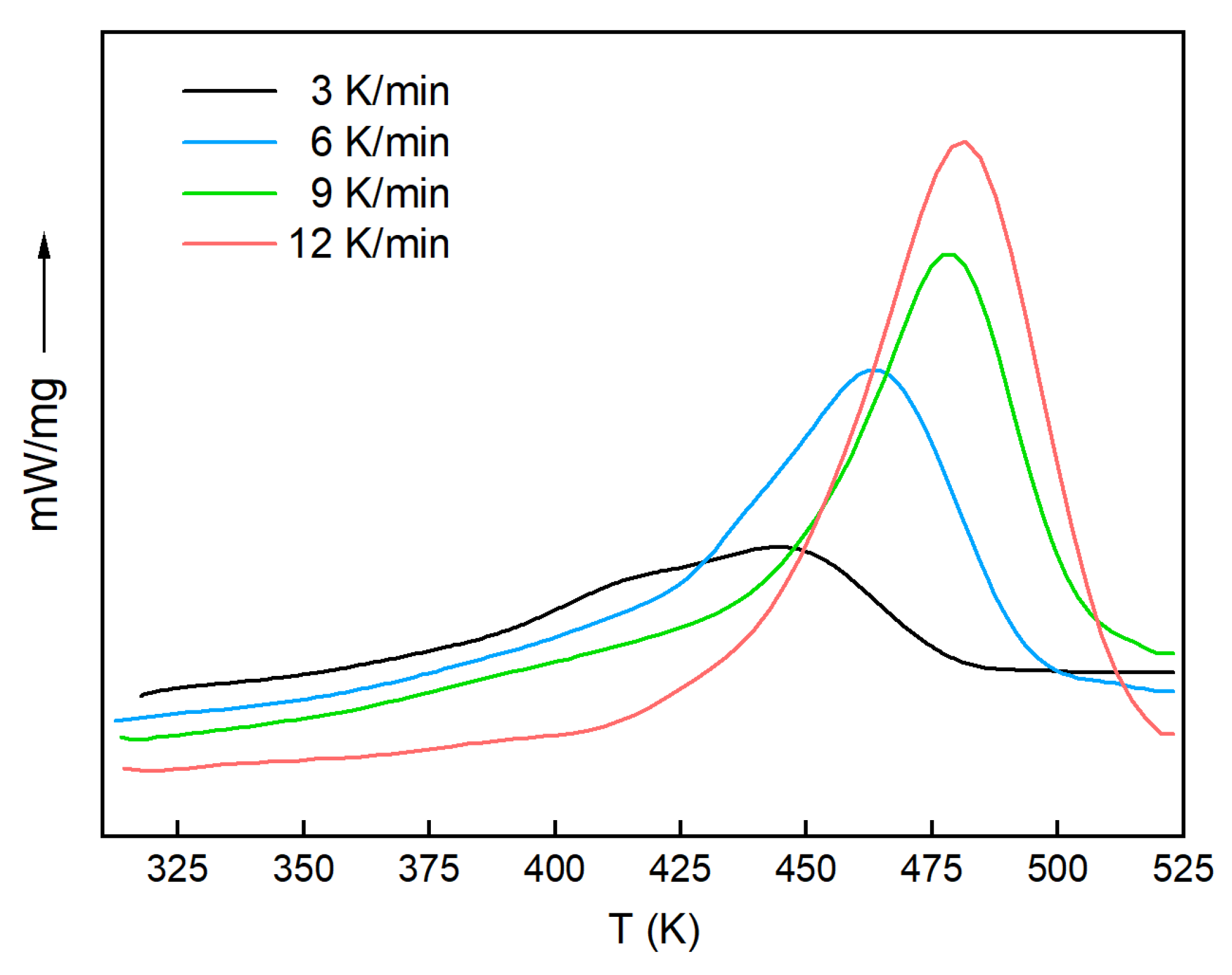
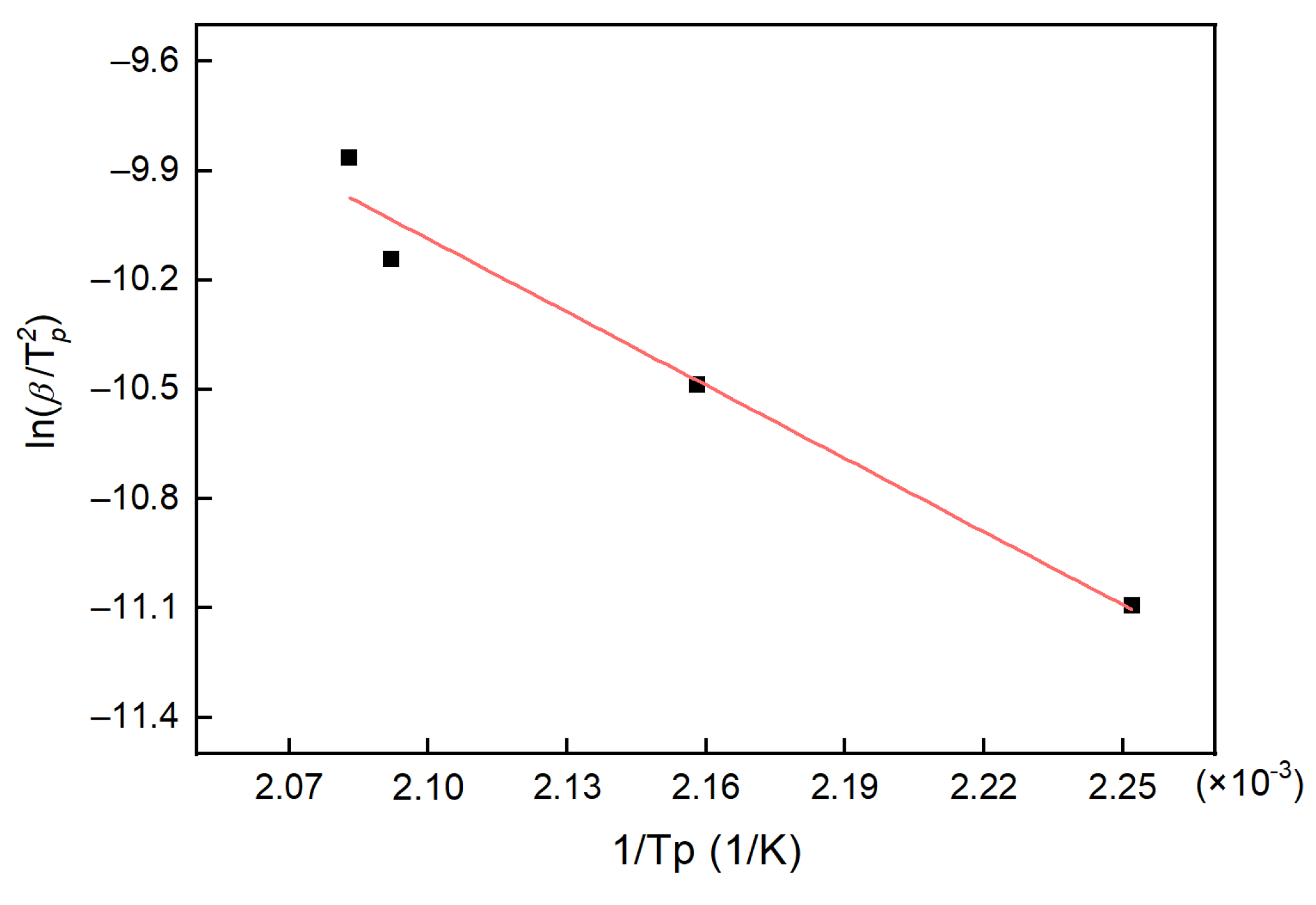
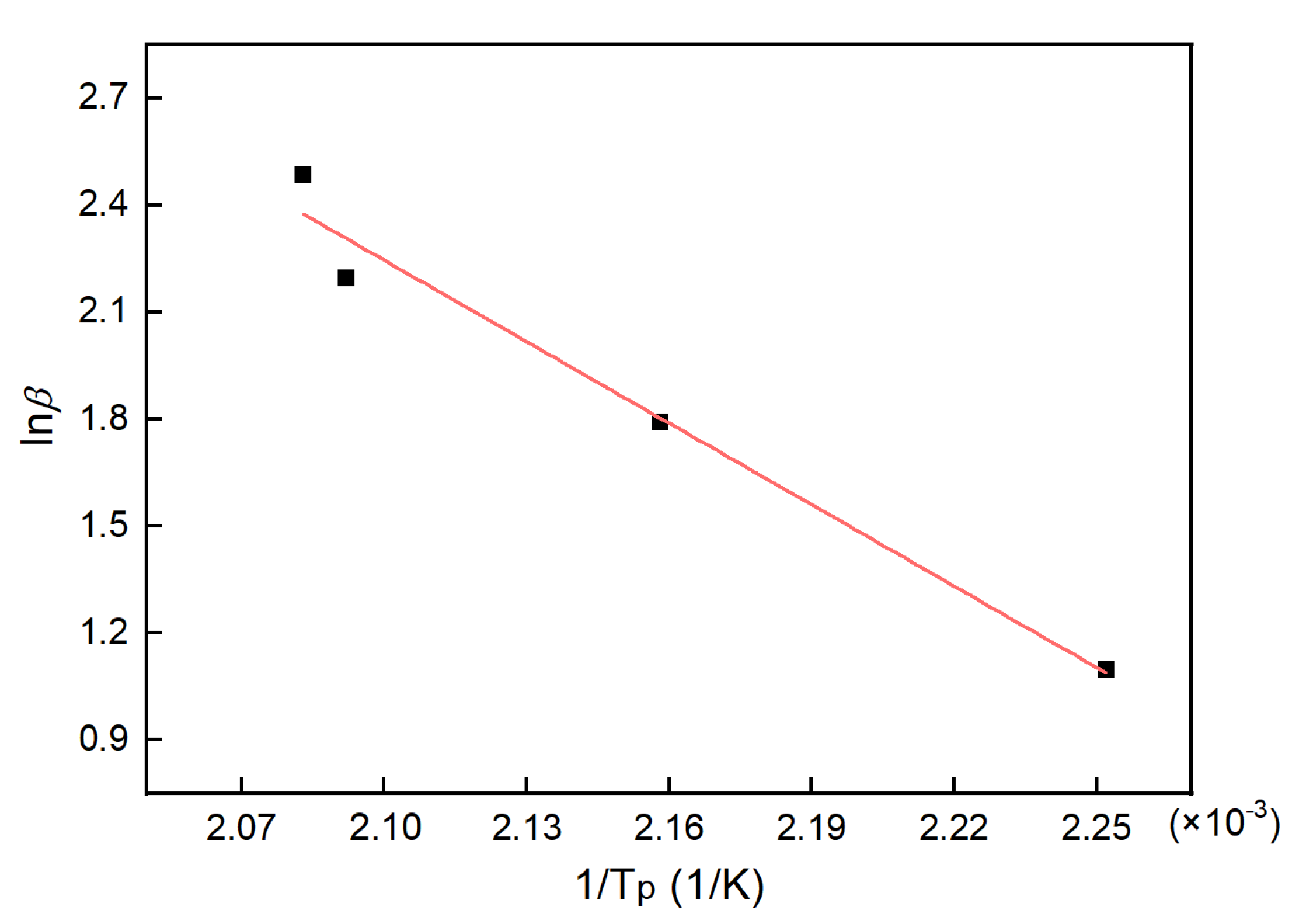
| β (K/min) | Tp (K) |
|---|---|
| 3 | 444.1 |
| 6 | 463.3 |
| 9 | 478.1 |
| 12 | 480.1 |
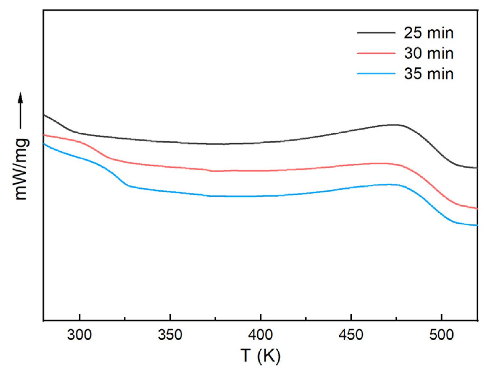
| Incubation Time | |||
|---|---|---|---|
| 25 min | 302.90 | 51.57 | 0.835 |
| 30 min | 310.00 | 34.52 | 0.890 |
| 35 min | 321.24 | 28.08 | 0.910 |
| Temperature (K) | Gelation Time (min) |
|---|---|
| 423 | 11.416 |
| 433 | 9.040 |
| 443 | 6.800 |
| T (K) | |
|---|---|
| 423 | 0.1939 |
| 433 | 0.1465 |
| 443 | 0.1100 |
| T/K | K | |
|---|---|---|
| 423 | 0.02735 | 1.56517 × 10⁻⁵ |
| 433 | 0.03050 | 2.20617 × 10⁻⁵ |
| 443 | 0.03639 | 3.06199 × 10⁻⁵ |
Publisher’s Note: MDPI stays neutral with regard to jurisdictional claims in published maps and institutional affiliations. |
© 2021 by the authors. Licensee MDPI, Basel, Switzerland. This article is an open access article distributed under the terms and conditions of the Creative Commons Attribution (CC BY) license (https://creativecommons.org/licenses/by/4.0/).
Share and Cite
Huang, S.; Zhang, G.; Du, W.; Chen, H. Construction of a TTT-η Diagram of High-Refractive Polyurethane Based on Curing Kinetics. Polymers 2021, 13, 3474. https://doi.org/10.3390/polym13203474
Huang S, Zhang G, Du W, Chen H. Construction of a TTT-η Diagram of High-Refractive Polyurethane Based on Curing Kinetics. Polymers. 2021; 13(20):3474. https://doi.org/10.3390/polym13203474
Chicago/Turabian StyleHuang, Shidi, Guiming Zhang, Weiping Du, and Huifang Chen. 2021. "Construction of a TTT-η Diagram of High-Refractive Polyurethane Based on Curing Kinetics" Polymers 13, no. 20: 3474. https://doi.org/10.3390/polym13203474