Characterizing Hyperspectral Microscope Imagery for Classification of Blueberry Firmness with Deep Learning Methods

Abstract

Firmness is an important quality indicator of blueberries. Firmness loss (or softening) of postharvest blueberries has posed a challenge in its shelf-life quality control and can be delineated with its microstructural changes. To investigate spatial and spectral characteristics of microstructures based on firmness, hyperspectral microscope imaging (HMI) was employed for this study. The mesocarp area with 20× magnification of blueberries was selectively imaged with a Fabry–Perot interferometer HMI system of 400–1000 nm wavelengths, resulting in 281 hypercubes of parenchyma cells in a resolution of 968 × 608 × 300 pixels. After properly processing each hypercube of parenchyma cells in a blueberry, the cell image with different firmness was examined based on parenchyma cell shape, cell wall segment, cell-to-cell adhesion, and size of intercellular spaces. Spectral cell characteristics of firmness were also sought based on the spectral profile of cell walls with different image preprocessing methods. The study found that softer blueberries (1.96–3.92 N) had more irregular cell shapes, lost cell-to-cell adhesion, loosened and round cell wall segments, large intercellular spaces, and cell wall colors that were more red than the firm blueberries (6.86–8.83 N). Even though berry-to-berry (or image-to-image) variations of the characteristics turned out large, the deep learning model with spatial and spectral features of blueberry cells demonstrated the potential for blueberry firmness classification with Matthew’s correlation coefficient of 73.4% and accuracy of 85% for test set.

1. Introduction

Firmness is an important quality factor of blueberries [1]. Regular intake of blueberries and their anthocyanin pigments not only provide a part of low-calorie meals but also reduce the risk of cardiovascular disease and type 2 diabetes as well as enhance neuroprotection [2]. For these reasons, international demand and supply of blueberries have reached an all-time high in recent years. The United States has been the top blueberry growing country in the world [3] and yielded 680 million pounds of blueberries accounting for $758 million in 2019 [4].

As blueberries are highly perishable, their quality upon arrival to final markets has major relevance to economic returns [5]. Dehydrated and soft blueberries are common defects of blueberries, [6] and blueberries are also susceptible to mechanical damage, as an injured berry loses its firmness and eventually reduces its quality and shelf-life [7]. Indeed, blueberry quality is a combination of appearance and flavor related to the degree of ripeness and firmness [8]. Usually, a blueberry is categorized into one of the three classes, firm, ripe, and overripe. The categories indicate that a firm berry yields to moderate pressure, and a ripe berry yields to slight pressure. An overripe berry is the one too soft and does not meet the grade requirements [8].

Firmness measurement for blueberries has been challenging as there was no standard method for firmness testing. A traditional way to measure the firmness was sensory evaluation in which an examiner rolled each berry with his/her fingers to rate its firmness, for example, with a 0–5 scale [9]. Because this conventional method was subjective and variable, several instrumental methods were proposed using equipment such as the Instron (Instron Corp., Norwood, MA, USA), FirmTech (BioWorks Inc., New York, NY, USA), and TA-XT (Stable Micro System Ltd., Godalming, UK) [10,11,12]. Most instruments measured compressing force required to deform the fruit surface for objective firmness evaluation but destroyed the fruit in the measurement process. An alternative method for firmness measurement was predicting the firmness without mechanical contact using a laser air-puff [13]. The instrument provided a new texture index for blueberry elasticity evaluation [11]. Blueberry growers often use an automated measurement device such as the FirmTech. Also, a durometer, which can be manual or automated, measures fruit firmness on a scale of 0 to 100, with 100 indicating the hardest [14].

There has been research to delineate the softening with microstructural changes of blueberries [1], which revealed that softer blueberries tend to lose cell-to-cell adhesion of parenchyma cells and likely have anthocyanin pigment bleeding from the epidermis and hypodermis layers. The previous studies implied that spatial and spectral features of blueberry cells could be good indicators of blueberry softening.

In this study, we investigated spectral and spatial features of the microstructures together for blueberry firmness classification using hyperspectral microscope imaging (HMI) and deep learning (DL). HMI has been viewed as an extension of color microscope imaging (CMI) for greater spectral detail. While an RGB image from CMI consists of three broad and overlapped bands displaying detected light of visible wavelengths 400–750 nm together, a hypercube from HMI contains a lot of narrow contiguous bands (e.g., 100–500 bands), each of which discloses spatial light distribution with a short range of wavelengths (e.g., 400–402 nm) [15]. HMI was used for this study to accurately examine both spectral and spatial dimensions of microstructures in 3D hyperspectral images. DL is a coined term for machine learning (ML) with modernized multilayer neural networks (MNN) [16,17,18]. The flexible data models have been successful in outperforming conventional machine learning methods and human experts in many applications, especially computer vision since early 2010 when mature technologies resolved or reduced many originating problems of MNN, such as heavy computation requirements, local optimum, a vanishing and exploding gradient, and a lack of tools such as DL software framework [16]. This study employed DL because it allowed different formats of inputs (e.g., images and spectra) for the model, flexible model design schemes against overfitting and underfitting, and generally, a better classification accuracy than conventional ML methods do [17,18].

The main goal of this study was to develop HMI methods for understanding blueberry softening. Specific objectives were to (1) acquire hyperspectral images of cells in blueberries, (2) analyze the hypercubes to find spatial and spectral relationships between blueberry firmness and microstructural changes, and (3) develop classification models with machine learning and DL methods. The results of this study would answer whether spectra and images of blueberry parenchyma cells from HMI are sound predictors for firmness classification and whether a DL model with the features can classify the firmness of a blueberry accurately.

2. Materials and Methods

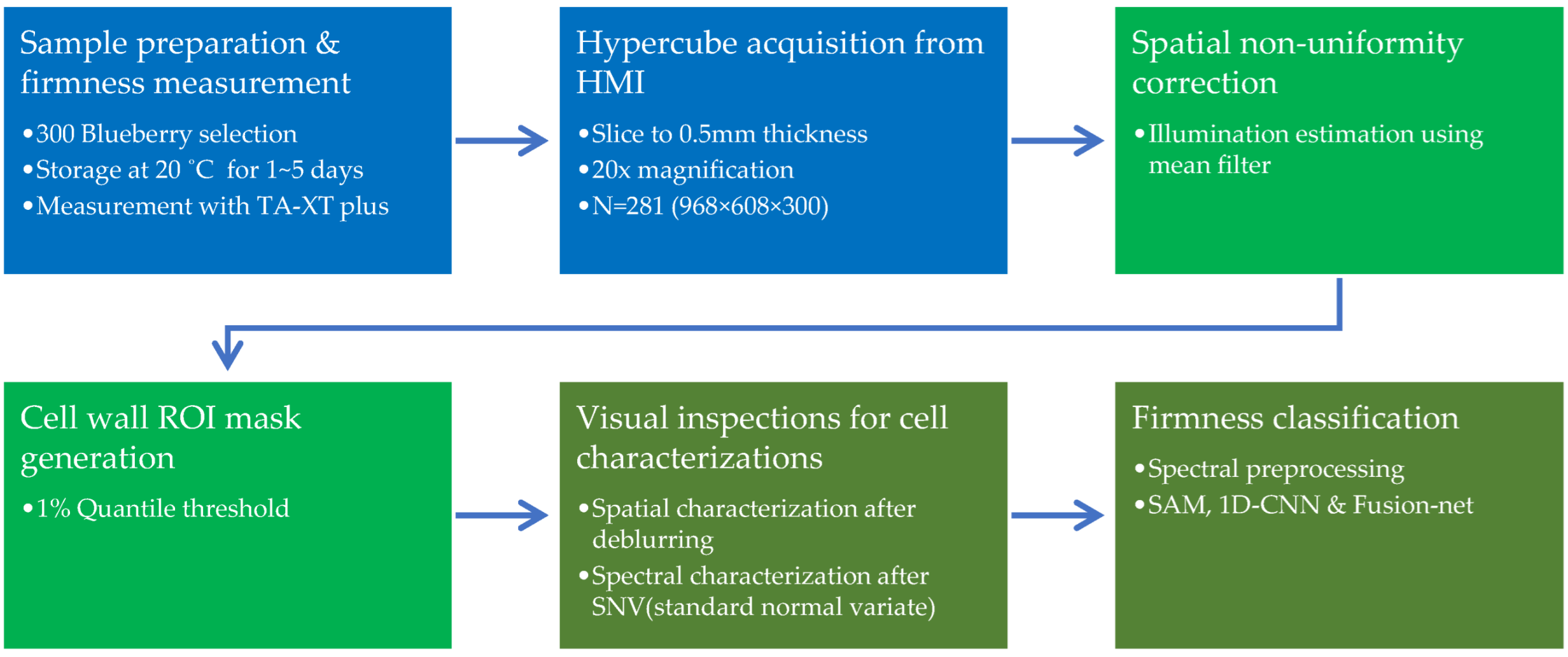
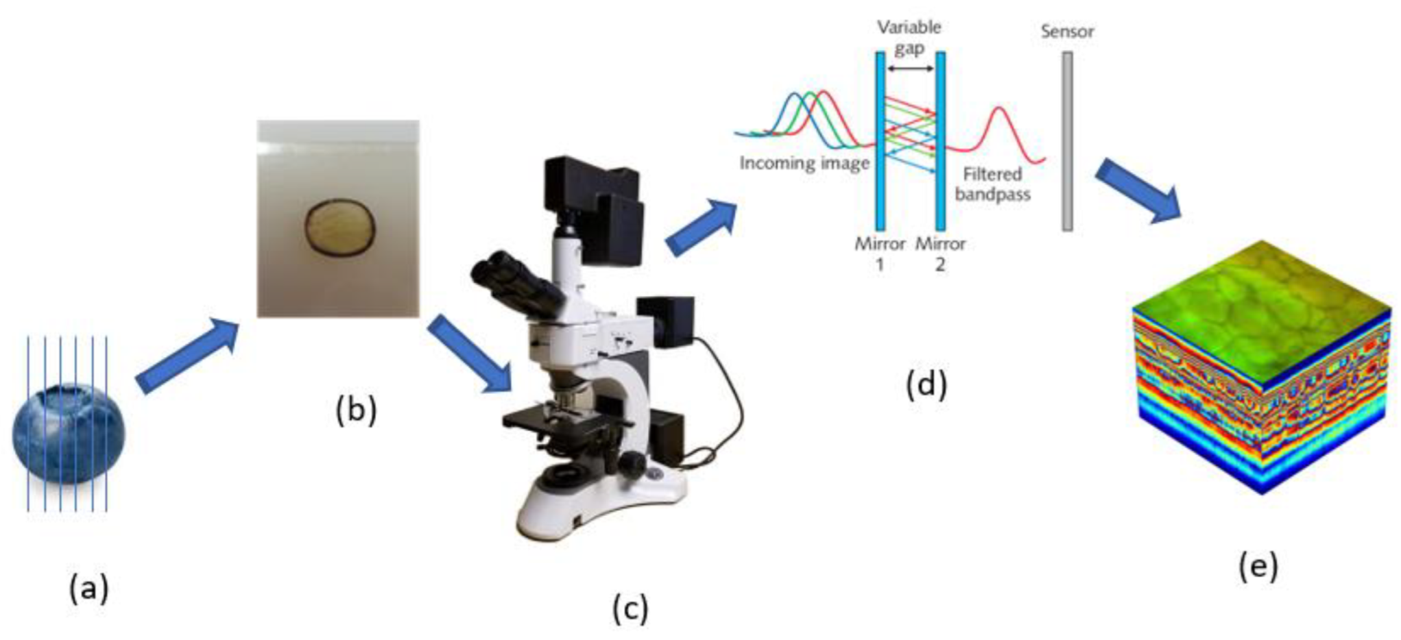
2.1. Summary Pipeline of Approaches

As shown in Figure 1, our approaches for this study included sample preparation, firmness measurement for ground-truth blueberry firmness, and hyperspectral image (hypercube) acquisition with HMI. The next step was image and data preprocessing for spatial non-uniformity correction and mask generation of cell wall regions of interests (ROI). The last step involved visual inspections for cell characterization, and firmness classification.

2.2. Sample Preparation and Firmness Measurement

For the blueberry microscope imaging, 300 intact blueberries were chosen from each of the two harvest regions (U.S. and Mexico) and stored at 20 °C with several different storage duration (e.g., one to five days). In brief, Figure 2 shows the schematic of the sample preparation and hyperspectral microscopic image measurement.

After the storage period specific for each blueberry, its firmness was assessed using a TA-XT plus Texture Analyzer, operated with Texture Exponent software (Version 4.0.13.0, Texture Technologies Corp., Scarsdale, NY, USA). The instrumental texture measurement employed puncture analysis on intact blueberries. The texture analyzer was equipped with a 50 kg load cell, and a blueberry was placed between a cylindrical puncture probe of 5 mm diameter and a cylindrical stainless flat platform with the blueberry calyx end facing vertically toward the probe. The blueberry was punctured to 5 mm with 5 g auto force trigger and 1.7 mm/s test speed. The measurements on 300 blueberries produced force max, max force strain, force linear distance, final force, and force area for each blueberry [19]. Shear force (SF) maximum (or force max) in each measurement was recorded in gram (g) and converted to Newton (N) to represent each blueberry firmness.

2.3. Hyperspectral Microscope Imaging

Then, the blueberry was sliced to 0.5 mm thickness with a razor to prepare its microscope slide as shown in Figure 2b. The hyperspectral microscope imaging (HMI) on the blueberry slices produced 281 hypercubes (132 from U.S. and 149 from Mexico) of parenchyma cells with a dimension of 968 × 608 × 300 (width × height × bands) in voxels. Each transmittance hypercube of parenchyma cells in the blueberry slice was acquired with a Fabry–Perot interferometer (FPI) HMI system (4200M, HinaLea, Emeryville, CA, USA). The imaging system consisted of an FPI spectrometer, an upright microscope (Amscope, Irvine, CA, USA), a palm-size PC with Intel Core i7 CPU, Linux OS, and image acquisition software (Truscope, HinaLea, Emeryville, CA, USA). The image spatial resolution was 968 × 608 in pixels, and the spectral range was 400–1000 nm, generating 300 spectral bands with a spectral resolution of 2 nm (FWHM). The imaging system was prepared with tungsten halogen illumination and 20× objective lens. In addition to dark calibration against image sensor errors, spectral (or wavelength) and radiometric calibration for accurate and stable HMI were carried out to normalize the output spectra from the HMI based on reference imaging using a multi-ion discharge lamp (LightForm Inc., Ashville, NC, USA) and a standard yield lamp for photonic calibration (SYLPH) (LightForm Inc., Ashville, NC, USA) [20]. All 281 hypercubes were finally obtained with 200 ms exposure time and 16.7% gain for further image processing.

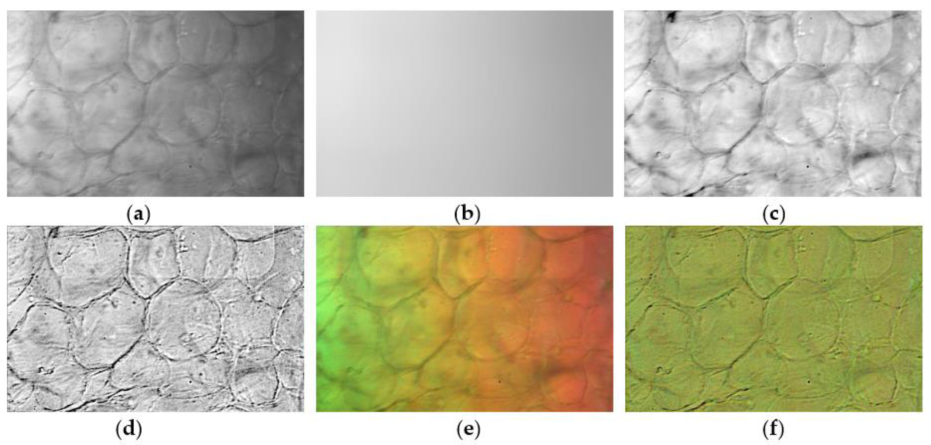
2.4. Hypercube Processing

Before hyperspectral analysis with the image data, each hypercube was examined with ENVI software (version 5.6, Harris Geospatial Solutions, Broomfield, CO, USA) and processed using image processing techniques. The initial investigation revealed that the raw hypercubes had spatial non-uniformity throughout the bands collected. Yet, we were able to correct the non-uniformity with image processing techniques prior to processing the hypercubes to generate ROI mask images of cell walls as detailed in the next subsections.

2.4.1. Spatial Non-Uniformity Correction for Every Wavelength

The spatial non-uniformity of raw hypercubes was corrected with a series of image processing techniques. Figure 3a,e showed the spatial non-uniformity in a raw band image and three-band image (450 nm, 530 nm, and 680 nm) of a raw hypercube. To fix the non-uniformity, we estimated an image of non-uniformity intensity distribution for each band using a mean filter of a large size 300 × 300 (Figure 3b), and the estimated non-uniformity image was subtracted from the raw band image (Figure 3a) to remove the non-uniformity. To finalize the spatial non-uniformity (Figure 3c), we shifted all pixel values of the resulting band image so that their median value is equal to that of the raw band image to reserve spectral profiles in the raw hypercube. Figure 3d,f showed a result of deconvolution using a Gaussian filter with filter size 45 to reduce the blurriness of the resulting band image and three-band image for subsequent visual inspections. Our validation results showed that the non-uniformity correction reduced pixel variation (i.e., standard deviation of pixel intensities) up to 38% on average. The correction also increased spectral variation among firmness groups while improving the linear relationship between firmness and average intensity at each peak wavelength (530 nm and 680 nm). For example, the non-uniformity correction increased R² between firmness and average intensity from 79.0% to 87.2% at 530 nm and 72.1% to 81.4% at 630 nm.

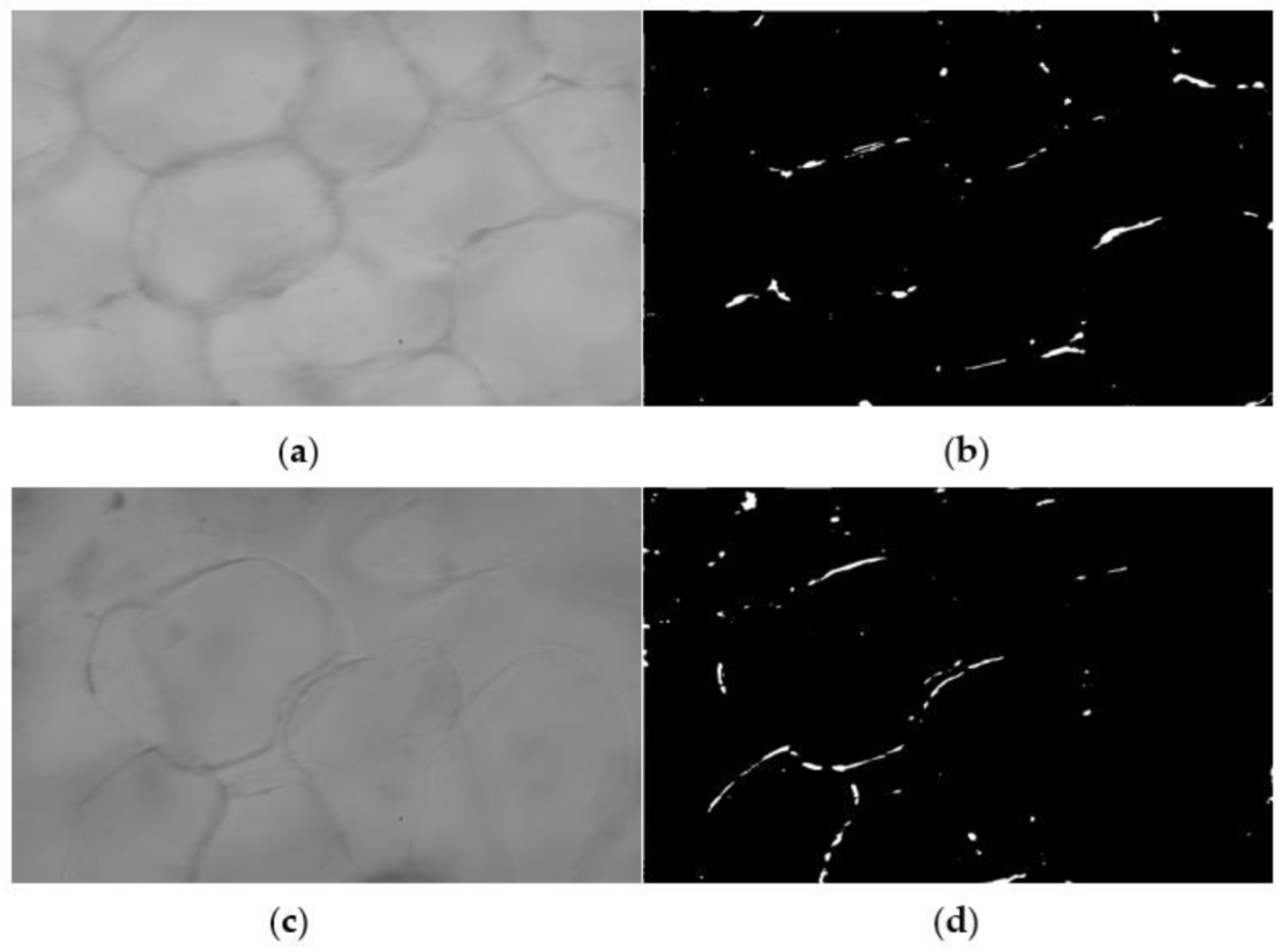
2.4.2. ROI Mask Generation of Cell Walls Using Quantile Threshold

After correcting the spatial non-uniformity in hypercubes, ROI masks of cell walls were generated using the quantile thresholding method [21]. To examine the spectra of parenchyma cell walls in blueberries, it was essential to create a proper ROI mask image of the cell walls for each hypercube. However, the initial inspection of the hypercubes presented some challenges because (a) the cells were nearly transparent, showing blurry cells behind, (b) many cells overlapped each other, (c) only a part of the cell wall around a cell was visible, and (d) different degrees of blurriness on different cell walls made it hard to recognize cell walls. Instead of engaging in time-consuming manual ROI mask generation, we utilized an improvised solution using quantile threshold because perfect or near-perfect precision of the cell wall ROIs was difficult even with manual mask image creation and was not a goal of this study. To create cell wall ROIs using quantile thresholding, we obtained 1% quantiles of average band images of peak wavelengths (530 nm and 680 nm) and thresholded the average band images with the 1% quantiles as shown in Figure 4. The threshold value 1% was chosen because ROIs with 1% had fewer artifacts from the cell walls behind foreground cells than those with 2% and 5%, and the average spectra between ROIs of 1% and 5% were not statistically different to characterize based on blueberry firmness.

2.5. Spatial and Spectral Cell Characterization on Blueberry Firmness

After properly processing hypercubes, parenchyma cells in blueberries were spatially and spectrally outlined based on blueberry firmness. For the cell characterization, greyscale images and spectra of cell walls were extracted from the hypercubes. We chose 530 nm band images for the spatial characterization because 530 nm was one of two peak wavelengths, and the band images showed less noise than the 680 nm band images did. After deblurring the band image of 530 nm with Gaussian filter [22], the spatial cell properties with different firmness were visually examined in terms of parenchyma cell shape, their cell wall segment, cell-to-cell adhesion, and size of intercellular spaces. After extracting spectra from hypercubes with the ROI mask images discussed in the previous section, we also investigated spectral cell characteristics based on average spectra per firmness group and per blueberry with different preprocessing methods (SNV, SNVD-DIFF7, and MSC-DIFF7) that are briefly introduced in the next section.

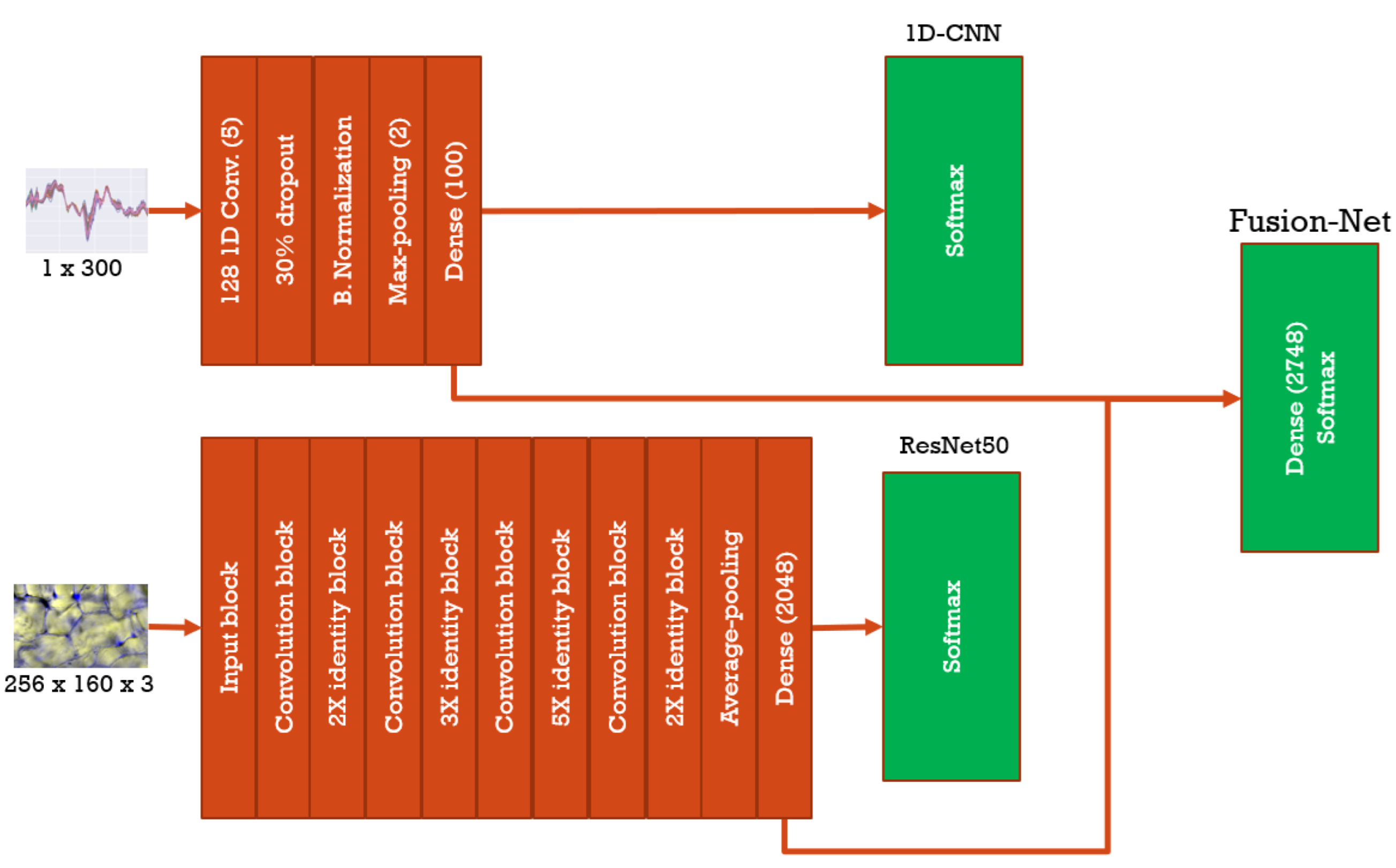
2.6. Firmness Classification

To confirm the results of spatial and spectral cell characterizations, we trained and evaluated machine learning and deep learning models using a PC with 3.8 GHz 12-core CPU, 64 GB memory, 1TB NVME hard disk, Nvidia RTX 2080 TI GPUs, and Windows 10. The PC was built with a liquid CPU cooling solution (CLC 280, EVGA Corp., Brea, CA, USA), five 12”-14” case fans and two blower-style GPUs (ASUS Computer International, Fremont, CA, USA) for adequate system cooling during deep learning with the GPUs staying at 85 °C on average. Before training a classification model, we determined two firmness categories with 1.96–3.92 N and 3.92–9.81 N based on spatial and spectral cell characteristics with different firmness. For the firmness classification, we used the first dataset (N = 132) and employed three classification models, spectral angle mapper on spectra, 1D-CNN on spectra, and Fusion-Net on spectra and custom three-channel images [23,24], as explained in the next subsection. A custom image for the Fusion-Net contained three channels of 530 nm, 680 nm band images, and their band ratio image (i.e., 530 nm/680 nm). The study also examined seven different preprocessing methods (SNV, SNVD-MA7, SNVD-DIFF7, SNVD-DIFF7-MA, MSC-MA7, MSC-DIFF7, MSC-DIFF7-MA7), where SNV stands for standard normal variate, MSC multiplicative scatter correction, -D (as in SNVD) detrending, DIFF7 first derivative with window size 7, and MA7 moving average with window size 7. We chose the seven combinations of preprocessing techniques among hundreds of possible candidates based on previous studies [25] and preliminary trials. Classification results were compared based on Matthew’s correlation coefficient (MCC) in addition to classification accuracy because the dataset had an imbalance of 34% and 66% over the two classes, and classification accuracy could overestimate the performance of a classifier with imbalanced datasets [26]. After hyperparameter optimization for each classification model, we repeated to train and evaluate the model 10–100 times, finding the best classification result.

Algorithm Implementations for Classification Models

All three classification models (i.e., spectral angle mapper, 1D-CNN, and Fusion-Net) were implemented with Python programming language (v3.7.7) and its numerous packages (e.g., Tensorflow, Keras, Hyperopt, Spectral, Pysptools, Numpy).

Spectral angle mapper (SAM) is a distance-based classification method on spectra with spectral angle distance [23]. Scripts for training (or computing reference spectra of each group) and evaluating SAM in our study were implemented using a Python package pysptools.

The DL classification algorithm on spectra [24] is 1D-CNN. The original architecture and implementation from [24] were modified based on the blueberry dataset and subsequent hyperparameter optimizations using the tree-structured parzen estimator (TPE) method [27]. The upper part of Figure 5 shows the architecture of 1D-CNN. The network started with a 1D convolutional layer with 128 filters of filter size 5, went through the dropout layer of 30% dropout rate, batch normalization layer, and max-pooling of pool size 2, before the dense (or fully connected) layer of 100 units and the final softmax layer for the classification operation [17]. Also, the learning rate of 0.001 and a batch size of one were chosen for the model to prevent overfitting because of the small sample size. Our TPE optimization results showed that the small sample size was the main cause for overfitted models with other values of the hyperparameters. With a large sample size, the difference between training accuracy and validation accuracy was often reduced by lowering model complexity (e.g., number of units or number of layers) and introducing regularization and a higher dropout rate. However, the small sample size made it difficult to adjust those hyperparameters against overfitting because of the limited choices and unsatisfactory results (i.e., overfitted model or low accuracy). The study found that the most effective strategy against overfitting with a small sample size was training the model with the smallest batch size and the other hyperparameters obtained from the TPE optimization with the fixed batch size. Because of the small batch size, training the model took about 3 min.

Fusion-Net is another deep learning algorithm on multiple forms of predictors [27]. For example, the original algorithm accepted three different forms of predictors, such as spectra, morphological properties, and greyscale images in our study. We modified its architecture and implementation for a Fusion-Net model of firmness classification on two forms of predictors (i.e., spectra and three-band images), as shown in Figure 5. The Fusion-Net consisted of 1D-CNN and ResNet50 without their last softmax layers. The last layers of the two subnetworks were combined with a dense (or fully connected) layer of 2748 units before the final softmax layer of the Fusion-Net. ResNet50 was one of the popular DL models for image classification, partly because the model resolved the vanishing gradient problem, causing more complex networks to learn less by employing skip or near-skip connections within identity and convolutional blocks [28,29]. Except for input-related settings (e.g., image dimensions) and overfitting-related parameters (e.g., batch size, drop rate, and learning rate), most hyperparameters of ResNet50 from [28] were retained in Fusion-Net. Like 1D-CNN, critical hyperparameters of the model were obtained through multiple trials of model training and evaluation using the TPE method with the fixed batch size 1, before building the final Fusion-Net model. Training the model took about 12 min.

3. Results

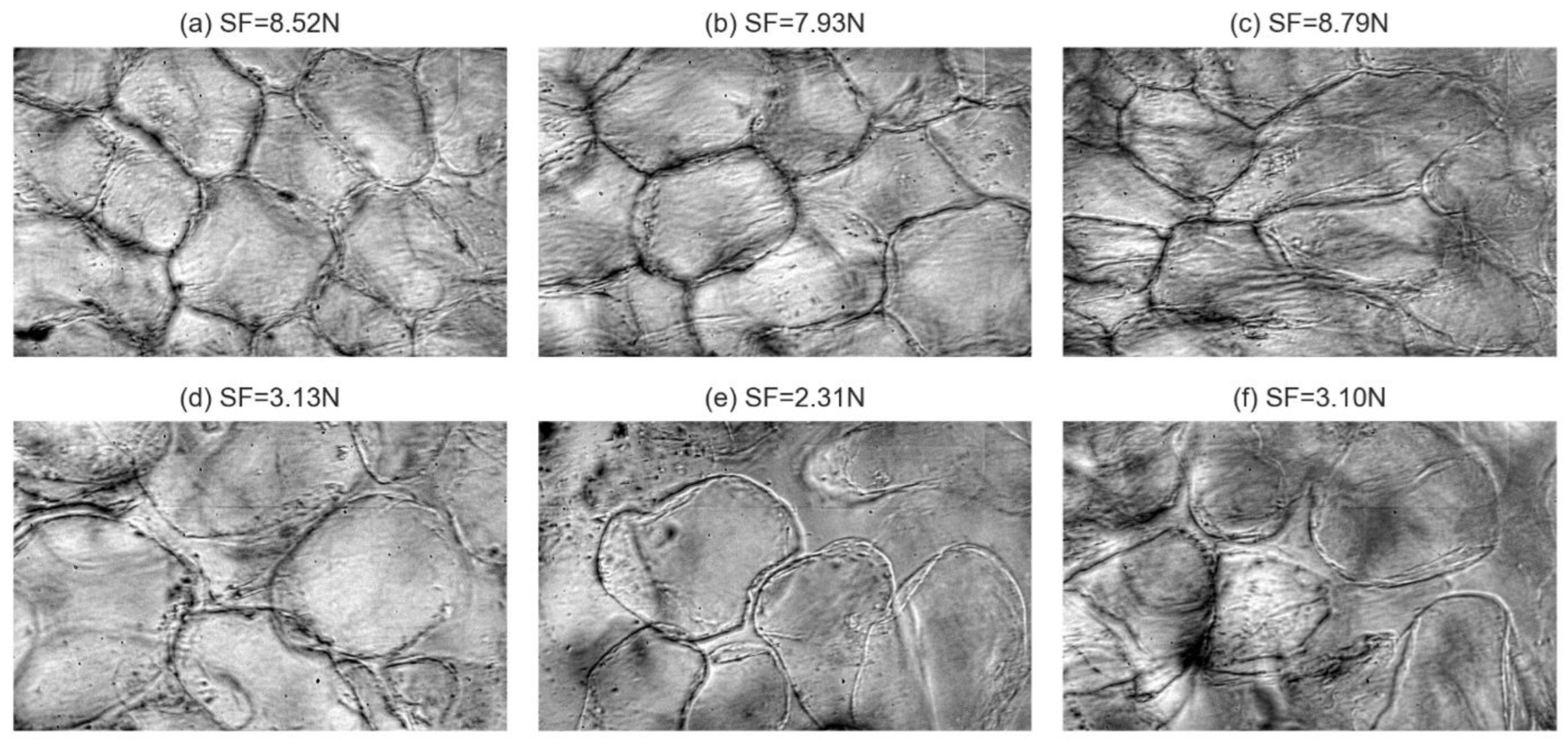
3.1. Spatial Cell Characteristics Based on Firmness

A deblurred 530 nm image was examined for spatial cell characteristics based on different firmness. Figure 6 showed the image patterns of parenchyma cells in the firmest blueberries (SF 7.85–8.83 N, (a)–(c)), and in the softest (SF 1.96–3.92 N, (d)–(f)) harvested from the United States. Most cells in the firm blueberries had tight cell-to-cell adhesions, thick, dark, and stiff (or straight) cell wall segments, and small intercellular spaces. In addition, variation of cell area was relatively small for the firm blueberries. Some cells in the soft blueberries lost cell-to-cell adhesions, had thin, light, and loosened (or round) cell wall segments while showing large intercellular spaces. Accordingly, overlapping cells and irregular cell shapes were also visible, while cell area variation appeared high for the soft blueberries.

However, the spatial cell characteristics for different firmness were not consistently noticeable for every blueberry because of considerable image-to-image variation and subtle microstructural changes. For instance, some images of soft blueberries (SF 1.96–3.92 N) did not display lost cell-to-cell adhesions, large intercellular spaces, nor large variations in cell areas. However, further inspection of images indicated that the sizeable between-image variation was related to sub-optimal imaging parameters such as imaging location, field of view (FOV), and magnification. This variation source and its possible solutions were explained in the Discussion section.

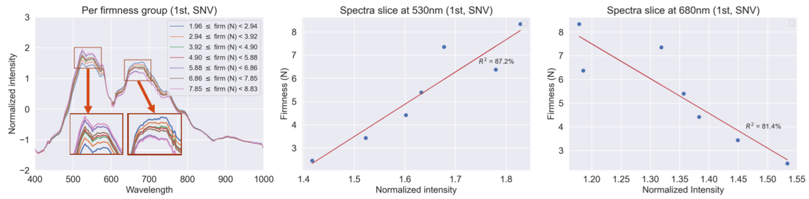
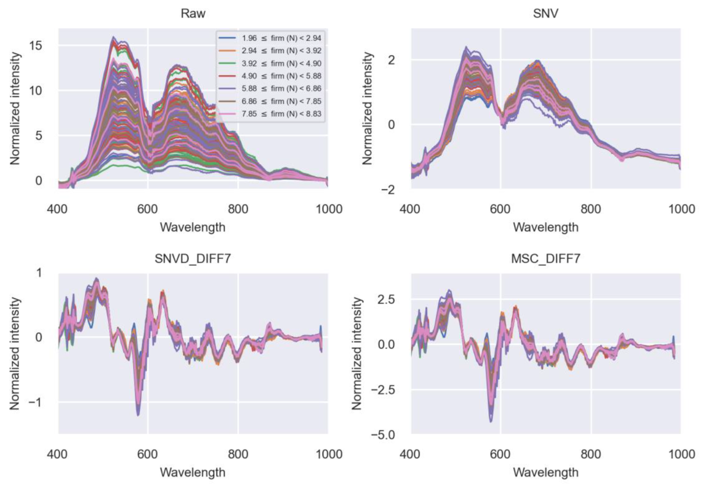
3.2. Spectral Cell Characteristics Based on Firmness

Average spectra of parenchyma cell walls in blueberries were preprocessed with SNV (standard normal variate) and drawn based on different firmness with a 0.98 N shear force interval in Figure 7. The relationship between the SNV-normalized average spectra and firmness was near-linear for softer blueberries (SF 1.96–4.90 N). For example, cell wall colors of blueberries with SF 1.96–2.94 N were redder and less green than those with SF 2.94–3.92 N, and to almost the same degree, those with SF 2.94–3.92 N were more magenta than those with SF 3.92–4.90 N. However, the cell wall colors of blueberries with more firmness (SF 4.90–8.83 N) did not have the near-linear relationship with firmness as the cell wall colors with SF 6.86–7.85 N were redder and less green than those with SF 5.88–6.86 N in blueberries. The nonlinearity probably showed a large variation of anthocyanin pigment bleeding in an early stage of microstructural change in blueberries.

The near-linear relationship of blueberry firmness with average spectra per firmness group was not obvious to recognize with average spectra per blueberry. Figure 8 shows average spectra per blueberry preprocessed with different methods (SNV, SNVD-DIFF7, MSC-DIFF7). Because of the large spectral variation among blueberries (or hypercubes), the effect from firmness was hardly visible even with SNV preprocessing. The other two preprocessing methods seemed to decrease the variation at most wavelengths but did not show any recognizable spectral trend over firmness.

3.3. Firmness Classification

To further examine the spatial and spectral characteristics for blueberry firmness, we trained and evaluated three different classification models on spectra and three-band images with seven preprocessing methods for spectra.

Table 1. Classification results of blueberry firmness from three classification models of SAM, 1D-CNN, and Fusion-Net with seven preprocessing methods. ACC and MCC indicate classification accuracy and Matthew’s correlation coefficient for the test set.

Preprocessing Methods	SAM		1D-CNN		Fusion-Net
	ACC (%)	MCC (%)	ACC (%)	MCC (%)	ACC (%)	MCC (%)
SNV	55	−2.3	80	54.5	80	56
SNVD-MA7	70	30.2	70	34.1	70	27.9
SNVD-DIFF7	70	31.3	65	0	80	54.5
SNVD-DIFF7-MA7	60	12.1	75	45.4	60	6.1
MSC-MA7	60	12.1	60	−1.5	70	39
MSC-DIFF7	70	30.3	85	66.3	85	73.4
MSC-DIFF7-MA7	60	−1.5	60	6.1	75	45.4

shows the classification results. The high variation of MCC over the different spectral preprocessing methods were noticeable. SAM with any preprocessing methods produced test MCC less than 35% and test accuracy less than or equal to 70%. However, 1D-CNN and Fusion-Net had better MCC than the SAM models did. Fusion-Net with MSC-DIFF7 turned out to be the best model with MCC of 73.4% and accuracy of 85%. Additionally, 1D-CNN with the same preprocessing method was the runner-up with MCC of 66.3% and accuracy of 85%. The two best models were trained with MSC-DIFF7-preprocessed spectra.

4. Discussion

This study was conducted (a) to investigate the feasibility of FPI HMI to classify blueberry firmness at the cellular level and (b) to understand how spatial and spectral changes of the cells are related to the softening. After processing each hypercube of parenchyma cells in the blueberries, the cell images with different firmness were visually examined based on the parenchyma cell shape, cell wall segment, cell-to-cell adhesion, and size of intercellular spaces. Spectral cell characteristics of the firmness were also sought according to the spectral profile of cell walls with various preprocessing methods. The study found that soft blueberries (SF 1.96–3.92 N) had more cells with irregular cell shapes, lost cell-to-cell adhesion, loosened and round cell wall segments, and large intercellular spaces, and its cell wall colors were less green and redder. But berry-to-berry variations of the characteristics turned out large. Even with the considerable variation in the cell characteristics for firmness, the spatial and spectral features of the cells (i.e., average spectra per blueberry and three-band images) showed their feasibility as a group of predictors for firmness classification with MCC of 73.4% and accuracy of 85% for the test set from Fusion-Net.

The second-best classification model was 1D-CNN with MSC-DIFF7 preprocessing on spectra with MCC of 66.3% and accuracy of 85%. It implies that adding spatial features (i.e., three-channel images) to spectral features only raised MCC by 7.1% without accuracy improvement. It means that the variation in spatial features could be relatively more considerable than that in spectral profiles.

The best model was interestingly achieved with MSC-DIFF7 preprocessing. It was difficult to visually classify firmness with MSC-DIFF7-processed spectra, but deep learning models seemed to find useful features in the preprocessed spectra.

In addition, we noticed large between-image variation in blueberry hypercubes. However, according to our subsequent investigation, it was concluded that those variations could be reduced by optimal parameters for imaging. For example, one was able to overcome the large berry-to-berry (or image-to-image) variation with a better strategy of imaging (e.g., imaging location, FOV, and magnification). Optimal FOV could be the one in which epidermis, hypodermis, and parenchyma cells are all visible because (1) anthocyanin pigment bleeding starts from the epidermis and hypodermis, and (2) moisture loss of parenchyma cells, a possible cause of blueberry softening and microstructural changes, more likely happens near the epidermis and hypodermis [1]. For the same reason, if it was challenging to include the epidermis and hypodermis in the FOV, a good alternative could be having parenchyma cells near the skin layer in the FOV. Magnifications of 5×–10× contain more parenchyma cells in the FOV and have less variation in average spectra per blueberry than 20×, as the results of our spectral study indicated. Those optimal parameters and thus, less between-image variation should improve the accuracy of the proposed classifier.

Comparing this study’s results with those of related research has been challenging because of the difference in firmness measurements and variability among blueberry cultivars. Even without considering different instruments to measure the firmness, researchers used different sizes of probes and weights of load cells for the measurements [30,31], and while some studies used maximum force to deform (e.g., N) as a firmness unit, the others force and probe travel distance required to deform (e.g., N/mm). In addition, our preliminary study confirmed that spatial and spectral changes of blueberry microstructures were distinct among different cultivars [1] and that training a separate classification model would be necessary for blueberries of another cultivar.

Although this study with HMI required cutting intact blueberries for the firmness classification, it must be reminded that this study and further studies with HMI may lead to development of a nondestructive method for the classification. For example, if our future studies with HMI uncovered spectral and spatial cell changes in blueberry skin over the blueberry softening, color or hyperspectral imaging equipped with a macro lens would help to nondestructively categorize the firmness of blueberries. As this study revealed the potential of HMI for blueberry firmness classification, further research with more data needs to be done to confirm those implications of the study.

The mention of trade names or commercial products in this article is solely for the purpose of providing specific information and does not imply recommendation or endorsement by the U.S. Department of Agriculture.

References

1. Allan-Wojtas, P.M.; Forney, C.F.; Carbyn, S.E.; Nicholas, K.U. Microstructural indicators of quality-related characteristics of blueberries—An integrated approach. LWT-Food Sci. Technol. 2001, 34, 23–32. [Google Scholar] [CrossRef]
2. Kalt, W.; Cassidy, A.; Howard, L.R.; Krikorian, R.; Stull, A.J.; Tremblay, F.; Zamora-Ros, R. Recent research on the health benefits of blueberries and their anthocyanins. Adv. Nutr. 2020, 11, 224–236. [Google Scholar] [CrossRef]
3. FAOUN. FAOSTAT. 2020. Available online: http://www.fao.org/faostat/en/#data/QC/visualize (accessed on 18 November 2020).
4. USDA. National Agricultural Statistics Service. 2020. Available online: https://www.nass.usda.gov/Statistics_by_Subject/result.php?CBDCF536-13A5-3D67-94CA-D068D478FBD4&sector=CROPS&group=FRUIT%20%26%20TREE%20NUTS&comm=BLUEBERRIES (accessed on 21 August 2020).
5. Retamales, J.B.; Palma, M.J.; Morales, Y.A.; Lobos, G.A.; Moggia, C.E.; Mena, C.A. Blueberry production in Chile: Current status and future developments. Rev. Bras. Frutic. 2014, 36, 58–67. [Google Scholar] [CrossRef] [Green Version]
6. Moggia, C.; Graell, J.; Lara, I.; Schmeda-Hirschmann, G.; Thomas-Valdés, S.; Lobos, G.A. Fruit characteristics and cuticle triterpenes as related to postharvest quality of highbush blueberries. Sci. Hortic. 2016, 211, 449–457. [Google Scholar] [CrossRef] [Green Version]
7. Xu, R.; Takeda, F.; Krewer, G.; Li, C. Measure of mechanical impacts in commercial blueberry packing lines and potential damage to blueberry fruit. Postharvest Biol. Technol. 2015, 110, 103–113. [Google Scholar] [CrossRef]
8. USDA; Agricultural Marketing Service. Fruit and Vegetable Programs: Blueberries—Shipping Point and Market Inspection Instructions. 2002. Available online: https://www.ams.usda.gov/sites/default/files/media/Blueberry_Inspection_Instructions%5B1%5D.pdf (accessed on 18 November 2020).
9. Sanford, K.A.; Lidster, P.D.; McRae, K.B.; Jackson, E.D.; Lawrence, R.A.; Stark, R.; Prange, R.K. Lowbush blueberry quality changes in response to mechanical damage and storage temperature. J. Am. Soc. Hortic. Sci. 1991, 116, 47–51. [Google Scholar] [CrossRef] [Green Version]
10. Silva, J.L.; Marroquin, E.; Matta, F.B.; Garner, J.O., Jr.; Stojanovic, J. Physicochemical, carbohydrate and sensory characteristics of highbush and rabbiteye blueberry cultivars. J. Sci. Food Agric. 2005, 85, 1815–1821. [Google Scholar] [CrossRef]
11. Li, C.; Luo, J.; MacLean, D. A novel instrument to delineate varietal and harvest effects on blueberry fruit texture during storage. J. Sci. Food Agric. 2011, 91, 1653–1658. [Google Scholar] [CrossRef]
12. Chen, H.; Cao, S.; Fang, X.; Mu, H.; Yang, H.; Wang, X.; Xu, Q.; Gao, H. Changes in fruit firmness, cell wall composition and cell wall degrading enzymes in postharvest blueberries during storage. Sci. Hortic. 2015, 188, 44–48. [Google Scholar] [CrossRef]
13. Prussia, S.E.; Astleford, J.J.; Hewlett, B.; Hung, Y.C. University of Georgia Research Foundation Inc. UGARF. Non-Destructive Firmness Measuring Device. U.S. Patent 5,372,030, 13 December 1994. [Google Scholar]
14. VSCNews. Methods for Measuring Fruit Firmness. 2019. Available online: https://vscnews.com/methods-for-measuring-fruit-firmness/ (accessed on 21 August 2020).
15. Park, B.; Yoon, S.C.; Lee, S.; Sundaram, J.; Windham, W.R.; Hinton, A., Jr.; Lawrence, K.C. Acousto-optic tunable filter hyperspectral microscope imaging method for characterizing spectra from foodborne pathogens. Trans. ASABE 2012, 55, 1997–2006. [Google Scholar] [CrossRef]
16. Kim, M.; Yun, J.; Cho, Y.; Shin, K.; Jang, R.; Bae, H.J.; Kim, N. Deep learning in medical imaging. Neurospine 2019, 16, 657. [Google Scholar] [CrossRef] [PubMed]
17. Goodfellow, I.; Bengio, Y.; Courville, A.; Bengio, Y. Deep Learning; MIT Press: Cambridge, UK, 2016. [Google Scholar]
18. Janiesch, C.; Zschech, P.; Heinrich, K. Machine learning and deep learning. Electron. Mark. 2021, 31, 685–695. [Google Scholar] [CrossRef]
19. Hu, M.H.; Dong, Q.L.; Liu, B.L.; Opara, U.L.; Chen, L. Estimating blueberry mechanical properties based on random frog selected hyperspectral data. Postharvest Biol. Technol. 2015, 106, 1–10. [Google Scholar] [CrossRef]
20. Eady, M.B.; Park, B.; Yoon, S.C.; Haidekker, M.A.; Lawrence, K.C. Methods for hyperspectral microscope calibration and spectra normalization from images of bacteria cells. Trans. ASABE 2018, 61, 438–448. [Google Scholar] [CrossRef]
21. Shih, F.Y. Image Processing and Pattern Recognition: Fundamentals and Techniques; John Wiley & Sons: Hoboken, NJ, USA, 2010; p. 120. [Google Scholar]
22. Gonzalez, R.C.; Woods, R.E. Digital Image Processing, 4th ed.; Pearson: New York, NY, USA, 2018; pp. 352–358. [Google Scholar]
23. Park, B.; Windham, W.R.; Lawrence, K.C.; Smith, D.P. Contaminant classification of poultry hyperspectral imagery using a spectral angle mapper algorithm. Biosyst. Eng. 2007, 96, 323–333. [Google Scholar] [CrossRef]
24. Kang, R.; Park, B.; Eady, M.; Ouyang, Q.; Chen, K. Classification of foodborne bacteria using hyperspectral microscope imaging technology coupled with convolutional neural networks. Appl. Microbiol. Biotechnol. 2020, 104, 3157–3166. [Google Scholar] [CrossRef] [PubMed]
25. Yoon, S.C.; Windham, W.R.; Ladely, S.R.; Heitschmidt, J.W.; Lawrence, K.C.; Park, B.; Narang, N.; Cray, W.C. Hyperspectral imaging for differentiating colonies of non-0157 Shiga-toxin producing Escherichia coli (STEC) serogroups on spread plates of pure cultures. J. Near Infrared Spectrosc. 2013, 21, 81–95. [Google Scholar] [CrossRef]
26. Chicco, D.; Jurman, G. The advantages of the Matthews correlation coefficient (MCC) over F1 score and accuracy in binary classification evaluation. BMC Genom. 2020, 21, 6. [Google Scholar] [CrossRef] [Green Version]
27. Kang, R.; Park, B.; Eady, M.; Ouyang, Q.; Chen, K. Single-cell classification of foodborne pathogens using hyperspectral microscope imaging coupled with deep learning frameworks. Sens. Actuators B Chem. 2020, 309, 127789. [Google Scholar] [CrossRef]
28. He, K.; Zhang, X.; Ren, S.; Sun, J. Deep residual learning for image recognition. In Proceedings of the IEEE Conference on Computer Vision and Pattern Recognition, Las Vegas, NV, USA, 27–30 June 2016; pp. 770–778. [Google Scholar]
29. Ji, Q.; Huang, J.; He, W.; Sun, Y. Optimized Deep Convolutional Neural Networks for Identification of Macular Diseases from Optical Coherence Tomography Images. Algorithms 2019, 12, 51. [Google Scholar] [CrossRef] [Green Version]
30. Schotsmans, W.; Molan, A.; MacKay, B. Controlled atmosphere storage of rabbiteye blueberries enhances postharvest quality aspects. Postharvest Biol. Technol. 2007, 44, 277–285. [Google Scholar] [CrossRef]
31. Paniagua, A.C.; East, A.R.; Hindmarsh, J.P.; Heyes, J. Moisture loss is the major cause of firmness change during postharvest storage of blueberry. Postharvest Biol. Technol. 2013, 79, 13–19. [Google Scholar] [CrossRef]
Figure 1. Summary pipeline of the blueberry firmness study.
Agronomy 12 00085 g001
Figure 2. Schematic of sample preparation and hyperspectral microscope image measurement. (a) Blueberry sample with cutting direction; (b) blueberry on slide for scanning; (c) hyperspectral microscope; (d) Fabry–Perot Interferometer (FPI) for acquiring hyperspectral data; (e) hypercube from blueberry sliced sample.
Agronomy 12 00085 g002
Figure 3. Non-uniformity correction of blueberry hyperspectral microscope images acquired by FPI-HMI at 530 nm: (a) raw image, (b) image from mean filter with filter size 300 × 300, (c) non-uniformity-corrected image, (d) deconvoluted and 1% linear stretched image, (e) raw three-band image, (f) deconvoluted three-band image after the correction.
Agronomy 12 00085 g003
Figure 4. Example of quantile thresholding (a) normalized average band image of 530 nm and 680 nm for a blueberry with firmness 7.93 N, (b) 1% quantile thresholding results from (a,c) normalized average band image for a blueberry with firmness 2.31 N, (d) 1% quantile thresholding results from (c).
Agronomy 12 00085 g004
Figure 5. Architectures of 1D-CNN and Fusion-Net; Fusion-Net combined 1D-CNN on spectra and ResNet50 on custom three-band images with three channels of 530 nm, 680 nm band images, and its band ratio image.
Agronomy 12 00085 g005
Figure 6. Parenchyma cells in blueberry fruit with different firmness; (ac) SF 7.85–8.83 N with tight cell-to-cell adhesion (CCA), thick, dark, and stiff cell walls (CW), small intercellular spaces (IS); (df) SF 1.96–3.92 N with more CCA lost, thinner, light, loosened CWs, very large IS.
Agronomy 12 00085 g006
Figure 7. Average spectra of cell walls among different firmness; two plots on the right side show a linear relationship between firmness and average intensity normalized with SNV at each peak wavelength (530 nm and 680 nm).
Agronomy 12 00085 g007
Figure 8. Average spectra of cell walls per blueberry among different firmness with three different preprocessing methods, Raw (top-left), SNV (top-right), SNVD-DIFF7 (bottom-left), and MSC-DIFF7 (bottom-right).
Agronomy 12 00085 g008