3.1. NSRP Calibration and Validation of the Stationary Version
First of all, the available datasets for Viterbo rain gauge were analyzed in terms of the following:
Application of MK test for times series covering the periods 1928–2000 and 1928–2015 for AMR (for Annual Precipitation, the investigated periods were 1916–2000 and 1916–2015). This double-check was aimed at testing the hypothesis of stationary process for periods of different length, and at quantifying the data number to be used for calibrating the stationary version of NSRP;
Goodness-of-fit for AMR series with EV1 distributions, which constitute a good approximation for AMR from NSRP synthetic data [
27], as also remarked in
Section 2.4.2. Consequently, a satisfactory EV1 fitting can clearly support the adoption of an NSRP model for the selected case study.
At this step of analysis, sub-hourly AMR series were not investigated, since the sample size has a limited time span (the data are observed since 1994), and the trend evaluation would not have been reliable.
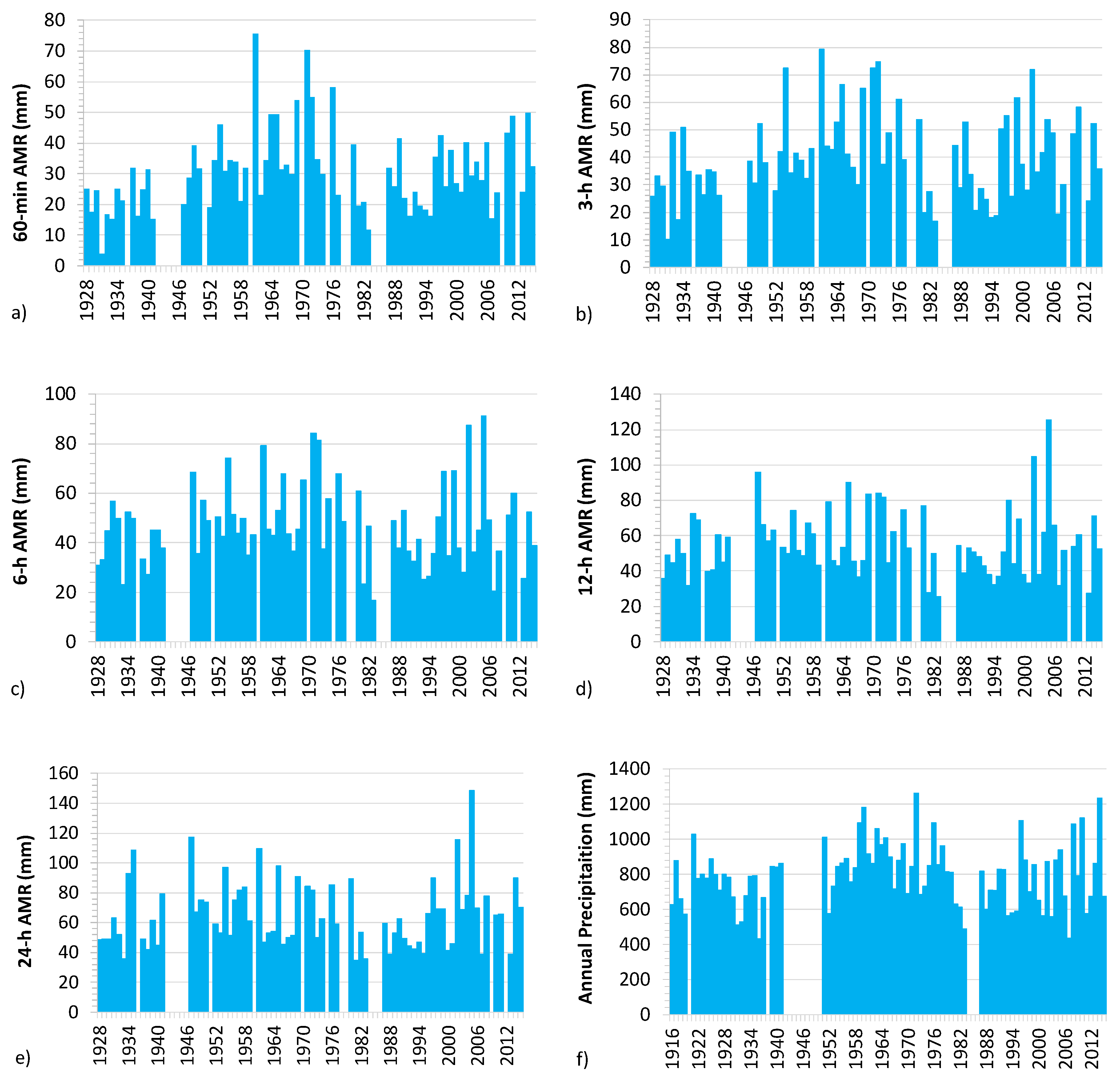
Chronological histograms for the investigated time series are reported in
Figure 3. Results from the MK test are schematized in
Table 1; the null hypothesis of no trend until 2015 cannot be rejected at 0.05 significance level for all the series, as
is less than 1.96 for all the samples, so the whole dataset can be used for calibration of the stationary model.
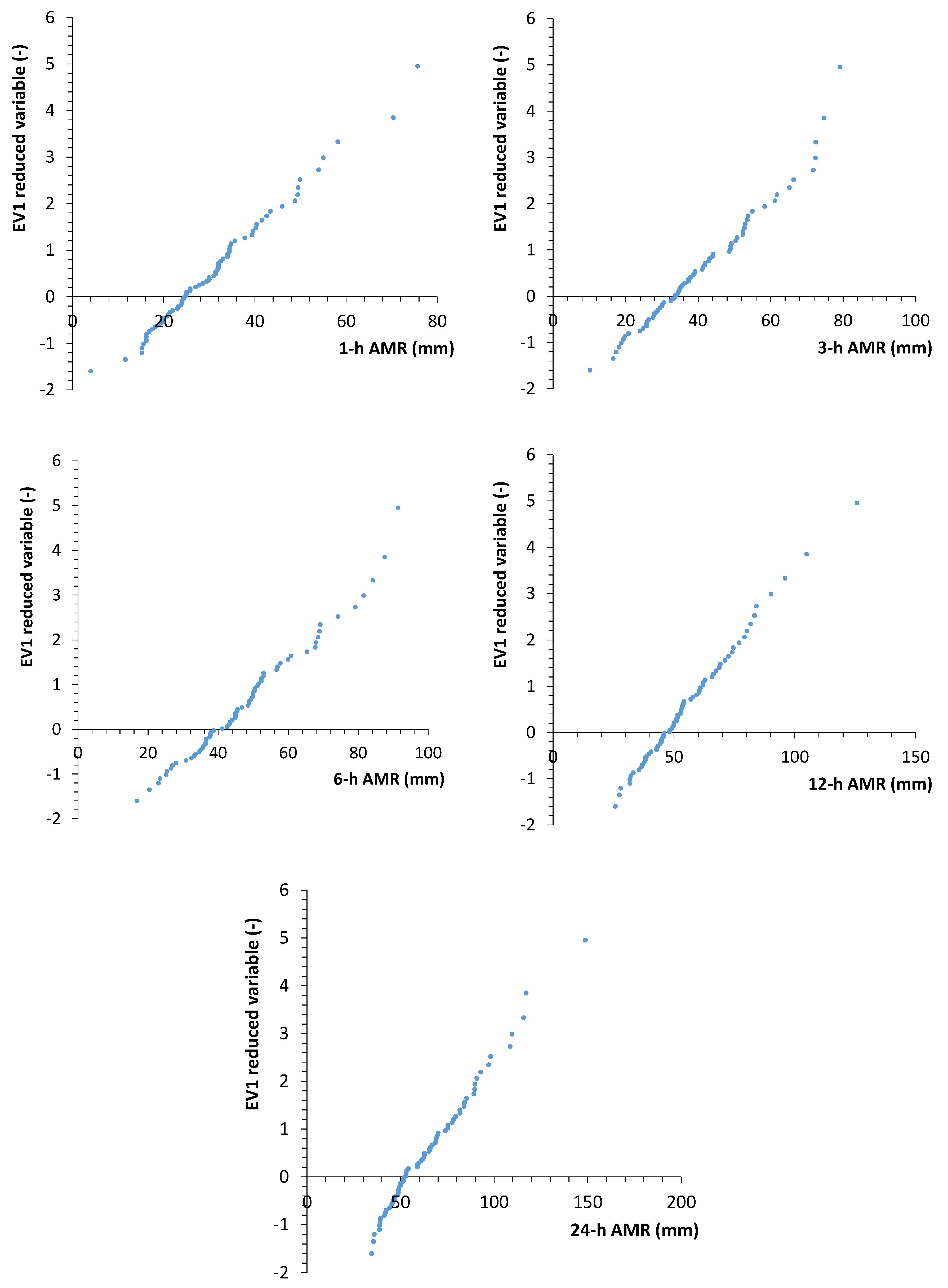
The EV1 probabilistic plots in
Figure 4 show the EV1 goodness-of-fit for the hourly AMR sample series, hence confirming the possibility to use the NSRP model.
As a second step, calibration of the stationary model was carried out as specified in
Section 2.2.1, and the results are shown in
Table 2. It can be noted that
assumes the value equal to π, which means that the mean waiting time 1/
λ(t) assumes the minimum value (
) when
t is very close to 0 and
Ty (i.e., in the winter period), while its maximum value occurs during the summer season. This result is coherent with the climatology of the Central and Southern Italy [
58].
The comparisons among average values for sample and NSRP AMR series (also including sub-hourly series, used for validation) and Annual Precipitation are reported in
Table 3.
Moreover, for validation, the comparisons among Amount–Duration–Frequency (ADF) curves obtained from the sample AMR series and those derived from the simulated continuous NSRP process were also carried out. Both sample and NSRP curves were calculated with the common two-parameters ADF formula:
where
AMRT(
d) is the annual maximum cumulative value for rainfall height (mm),
d is the rainfall duration (h), and
(mm/h) and
(-) are the ADF parameters related to return period
T, based on rain gauge observations.
Table 4 reports the estimates for
and
at prefixed values of return period
T for both cases. From
Figure 5 we can observe, by applying Equation (19) with parameters in
Table 4, a difference of about 2 mm for T = 20 years, about 0.9 mm for T = 50 years, about 0.1 mm per T = 100 years and about 0.6 mm for T = 200 years.
3.2. Results of Transient Version for the Proposed NSRP Model
As already mentioned in the Introduction, NSRP parameters are strongly related to finest scales, while RCM predictions are only available for coarser resolutions. Thus, some NSRP parameters trends were hypothesized, and the Authors considered those that provided compatible results with RCM scenarios, in terms of variation for maximum daily rainfall and annual precipitation. In detail, the adopted scenario combines the following hypotheses:
A linear increasing trend of 50% in 100 years concerning the mean value of Bursts Intensity (i.e., );
A linear decreasing trend of 25% in 100 years concerning the mean value of Bursts Duration (i.e., );
A linear increasing trend of 50% in 100 years concerning the mean waiting time between two consecutive storms (i.e., ).
These trends provided a marked variation, in terms of frequency distribution, for AMR series at finer resolutions (5 and 15 min) and for Annual Precipitation, while AMR series at coarser scales seem to be not so influenced by the imposed trends. Some comparisons are shown in
Figure 6, in which the frequency distributions for the initial year (t0) and the 25th (t25), the 50th (t50) and the 100th (t100) years are represented.
Focusing on Annual Precipitation (AP) and 24-h AMR series, the temporal evolution of their average values (calculated for each year from the correspondent 500 realizations), compatible with RCM projections, were characterized by the following (
Table 5):
A mean reduction of 82.5 mm in 100 years obtained for AP (well-matched with 71 mm in 90 years from RCP 8.5);
A slight increase for 24-h AMR, of about 4 mm in 100 years (the ensemble mean is, for both RCP 4.5 and RCP 8.5, up to 5–7 mm in 90 years, related to daily duration).
Moreover, from
Table 5, it can be noted that there is an increase in mean values of about 37% (5 min AMR), 28% (15 min AMR) and 17% (30 min AMR) in 100 years. These differences are lower and less evident for hourly timescales; indeed, the increase in average values is about 5–7% in 100 years.
The results can be justified from the assumed trend scenario:
An increase in burst intensity induces a clear marked effect (i.e., an expected increase in rainfall height) mainly for finer time resolutions (5–30 min), which are not so influenced by a contemporary reduction of burst duration.
On the contrary, for coarser resolutions (from 1 h), the simultaneous presence of an increase for intensity and of a reduction in bursts duration produces a sort of balance for rainfall heights, and then it is not possible to highlight a significant trend for AMR series.
The increase of the average waiting time between two consecutive storms mainly influences the reduction of annual precipitation, as expected from RCM projections.
This “scale effect”, i.e., that there are some particular time resolutions where the assumed temporal changes in parameters could be “hidden” when AMR series are studied, is also confirmed by analyzing the NSRP realizations with MK test.
The histograms in
Figure 7 indicate, for each investigated time resolution, the percentage of realizations with
Zs > 1.96. The percentages decrease, passing from a 5-min to 1-h time resolution, and are always less than 10% for hourly and multi-hourly AMR synthetic data. Concerning AP, the percentage with
Zs > 1.96 is about 30%.
The results from MK test highlight the importance of analysis with a SRG, and in particular with a large number of simulations. In fact, if a user would consider only one realization for all the investigated scales, he could obtain misleading assessments concerning the presence of trend or not for specific time resolutions. For example, if the considered 3-h AMR series belongs to the subset with Zs > 1.96, then the null hypothesis of no-trend is rejected; on the contrary, using a 15-min AMR series with Zs < 1.96 could imply the null hypothesis is not rejected. Similar considerations could be made if the application of MK test (or other similar tests) is carried out only on the observed series for a selected case study. Then, an overall analysis with a large number of simulations allows for a very in-depth investigation.
Concerning the variation of T-year percentiles and Hazard (
Section 2.4.2), the possibility of applying regression formulas for estimated EV1 parameters along the 100-year period was investigated. Coefficients for linear regressions are shown in
Table 6, together with the R
2 values, which are greater than 0.5, so that the obtained regressions can be considered as acceptable [
59]. As examples, the plots for 5- and 15-min EV1 parameters are illustrated in
Figure 8.
Then, the regression laws were used for quantifying the temporal variation of the following:
The 100-year and 200-year AMR quantiles with respect to the correspondent values
of the stationary process (
Figure 9);
Hazard (Equation (18)), by considering a 20-year moving time window (
Figure 10).
The increases are significant for finer resolutions, while they are relatively more limited, but still not negligible, for coarser scales. In details, increases for 24 h quantiles are 11–12% with respect to the stationary case, while they exceed 40% and 35% for the 5 and 15 min scales, respectively.
Hazard values, associated to a 20-year moving window and related to 100-year and 200-year quantiles of the stationary case, are as follows:
For finer scales (5–15 min), from 10% (T = 100 years) and 18% (T = 200 years) at the beginning of the investigated period, to 60% and 80%, respectively, at the end;
For 24 h resolutions, 20% (T = 100 years) and 35% (T = 200 years).
Thus, although variations for the investigated 24-h percentiles are relatively modest, the associated hazards at least double if compared with the values assumed at the beginning of the time horizon.
These results highlight the importance of investigation of several aspects before the choice of a stationary or a non-stationary model is made.
However, in a climate change context, it should be remarked the difference between the terms “stationarity” and “change”, and the fact that they are not mutually exclusive [
49]. Very popular “examples” can be mentioned [
49]. For instance, in the absence of an external force, the position of a body in motion changes in time but the velocity is unchanged (Newton’s first law). If a constant force is present, then the velocity changes but the acceleration is constant (Newton’s second law). If the force changes, e.g., the gravitational force with changing distance in planetary motion, the acceleration is no longer constant, but other invariant properties emerge, e.g., the angular momentum (Newton’s law of gravitation).
Non-stationarity is usually considered as synonymous with change, but change is a general notion applicable everywhere, including the real (material) world, while stationarity and non-stationarity are applied only to models, and not to the real world. Thus, environmental changes can be modeled also with stationary approaches [
60] and only in justified cases with non-stationary approaches.
In this specific case study, related to the Viterbo rain gauge in Central Italy, the imposed trends on
βI,
βD and
λ imply the need of using non stationary approaches for the finer time resolutions which are comparable with
βD and the annual aggregation (i.e., for MAP evaluation). This is true because a change on the inter-arrival time between two consecutive storms firstly influences monthly and yearly scales (
Figure 6).
On the contrary, a stationary modeling could be used for other investigated resolutions, as the temporal variation of the probability distributions seems not so significant. However, a complete analysis including the investigation of hazard and high percentiles makes the use of a non-stationary approach more plausible also for the coarser time resolutions.


