Article

Measuring on-Road Vehicle Hot Running NOx Emissions with a Combined Remote Sensing–Dynamometer Study

1
Department of Environment and Science, GPO Box 2454, Queensland Government, Brisbane, QLD 4001, Australia
2
Faculty of Engineering and Information Technology, University of Technology Sydney, Sydney, NSW 2007, Australia
3
Science and Engineering Faculty, Queensland University of Technology (QUT), Brisbane, QLD 4000, Australia
4
ARC Centre of Excellence for Mathematical and Statistical Frontiers (ACEMS), Queensland University of Technology (QUT), Brisbane, QLD 4000, Australia
*
Author to whom correspondence should be addressed.
Atmosphere 2020, 11(3), 294; https://doi.org/10.3390/atmos11030294
Submission received: 11 February 2020 / Revised: 4 March 2020 / Accepted: 10 March 2020 / Published: 16 March 2020
(This article belongs to the Special Issue Roadside Air Pollution)

Abstract

:
This study explores the correlation in measured hot running NO/CO2 ratios by a remote sensing device (RSD) and dynamometer testing. Two large diesel cars (E4/E5) are tested on the dynamometer in hot running conditions using a new drive cycle developed for this study and then driven multiple times past the RSD. A number of verification and correction steps are conducted for both the dynamometer and RSD data. A new time resolution adjustment of RSD acceleration values proves important. Comparison of RSD and dynamometer data consistently shows a strong weighted correlation varying from +0.89 to +0.95, despite the high level of variability observed in the RSD measurements. This provides further evidence that relative changes in mean NO/CO2 ratios as measured with the RSD should provide robust emissions data for trend analysis studies and as inputs for regional emissions models. However, a positive bias of approximately 25 ppm NO/% CO2 is observed for the RSD, and bias correction of RSD measurements should be considered pending further testing.

1. Introduction

Motor vehicles are a major source of air pollution and greenhouse gas (GHG) emissions in urban areas around the world. The close proximity of motor vehicles to the general population makes this a particularly relevant source from an exposure and health perspective [1].
Comprehensive measurement of vehicle emissions in urban networks is cost prohibitive due to the large number of on-road vehicles with different emission profiles, large spatial and temporal variability in vehicle activity and many real-world factors that influence emission levels. Instead, emission measurements are used to develop and validate vehicle emission (factor) models [2,3]. Models estimate emission loads at various scales, varying from local to global applications. Of particular interest is accurate quantification of on-road and real-world emissions. This information is essential for implementation of cost-effective measures to improve air quality in urban areas [4].
A range of methods is available to measure vehicle emissions. They include dynamometer and on-board emission measurements (PEMS), remote sensing, near-road air quality measurements and tunnel studies. However, all methods have their own strengths and weaknesses, and the weaknesses in particular must be clearly understood and explicitly considered in any subsequent use of emissions data, e.g., emission estimation and model validation [3].
The use of remote sensing to measure vehicle emissions is not new, dating back to 1971 [5]. Remote sensing devices (RSDs) have been used extensively for various purposes around the world including, but not limited to, identification of high-emitting vehicles, examination of on-road vehicle emissions distributions, trend analysis and model validation [5]. More recently, remote sensing has gained interest regarding measurement of real-world emissions and development of robust vehicle emission (e.g., [4,5,6,7,8]).
Given the increased use of remote sensing data and expansion of RSD data application, it is important to understand the level of association with other types of instrumentation. Strong correlation supports the combination of emission data sources, with or without correction for potential bias, whereas weak correlation suggests that further post-processing and correction may be required, if possible.
A recent study compared remote sensing with on-road air quality monitoring and found a weak (NO, nitrogen oxide) to significant (CO, carbon monoxide) weighted positive correlation in calm atmospheric conditions, and no significant correlation in other conditions [9]. Local dispersion and atmospheric chemistry processes, as well as urban background concentration levels, weakened the correlation between the RSD and air quality monitoring equipment. Following on, this paper examines the correlation between remote sensing and dynamometer NOx measurements for two recent technology diesel vehicles.
Previous RSD–dynamometer studies have reported different levels of correlation, varying from poor to good [4,10,11,12,13,14,15,16,17]. This variability is attributed to, e.g., differences in experimental design, differences in equipment used, different driving conditions, different levels of data aggregation and different assumptions.
Previous studies suggest that CO, HC (hydrocarbons) and NO RSD measurements generally follow the trends observed in dynamometer measurements, but that there is a substantial amount of scatter in the measurements. Substantial differences between remote sensing and laboratory measurements occur at the individual vehicle level, but aggregated emissions data is expected to yield reasonable agreement.
Older studies are likely less relevant, as remote sensing equipment has continued to evolve and improve over time. In addition, average fleet emissions have substantially reduced as time progressed, posing new challenges for remote sensing measurements. It is thus important to examine the correlation for modern vehicles.

2. Methods

2.1. Site Selection for the Remote Sensing Device

An on-road measurement campaign has been conducted at three locations in Brisbane, Australia [9,18,19]: a freeway on ramp (FWY, road gradient 2.9°), a heavily trafficked urban road (URB, road gradient 2.8°), and a commercial road in an industrial area (COM, road gradient 0.4°). The COM site (Figure 1) is selected for its different land use, fleet mix and driving conditions, but also because it is close to a dynamometer test facility. This allowed for a comparison between dynamometer testing and remote sensing measurement, which is the subject of this paper. The other sites are shown in Figure S1.1, Supporting Information.

2.2. Dynamometer Instruments and Procedures

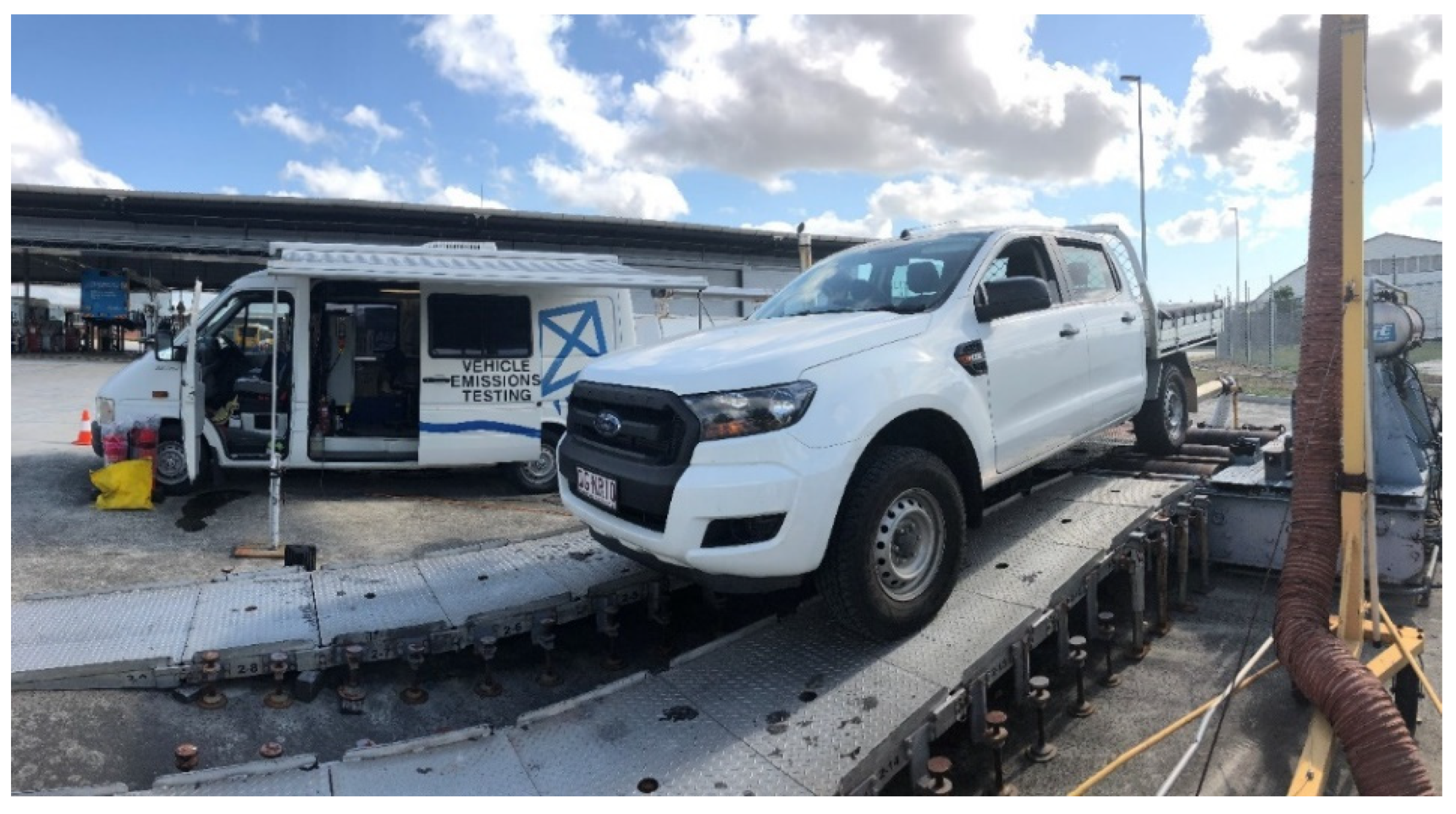
A chassis dynamometer is an instrument that simulates road loads according to a predefined speed–time profile (test or drive cycle) and load settings. During the test, exhaust concentration, the flow rate and the emission rate, as well as other variables such as speed, load and power, are measured and reported at a second-by-second time resolution. Figure 2 shows the dynamometer test set up with one of the test vehicles.
A portable transient vehicle dynamometer was used (Mustang Dynamometer, Model MD1000, Ohio, OH, USA). Dyno loading is achieved by two infinitely variable air-cooled Eddy current power absorbers, which are able to absorb power from the vehicle wheels up to 500 Hp (continuously) and 1200 Hp (peak). The Exhaust Gas Sampling and Analysis System (EGSAS) integrates laboratory grade instruments in one package. EGSAS includes a Horiba Model MEXA-720 (NOx), a California Analytical Instruments Model 602 (CO2, CH4) and a TSI DustTrak Aerosol Monitor Model 8250 (PM10). Ancillary equipment is included (Mid-West Instruments 301 Delta Tube Dilution Tunnel, Umwelt Technik Dilution Fan K52B and Schneider Electrical Microdrive Elite Variable Speed Drive or VSD).

2.3. Test Vehicles

Test vehicle 1 is a MY 2016 4WD Ford Ranger (Euro 4) with a 2.2 litre diesel engine, a diesel oxidation catalyst (DOC) and Exhaust Gas Recirculation (EGR). Test vehicle 2 is a MY 2017 4WD Ford Ranger (Euro 5) with a 3.2 litre diesel engine, a DOC, EGR and a diesel particulate filter (DPF). The vehicles are weighed on a weighing bridge before emission testing was conducted. It is noted that Euro 6 emission standards are not yet implemented in Australia, with a likely implementation year of 2027. Table 1 shows a summary of test vehicle specifications, as well as average dynamometer results, which will be discussed later.

2.4. Dynamometer Test Cycle

A dedicated test cycle is developed from Australian drive pattern data with the aim to create driving conditions that were similar to those encountered by a vehicle driving past the RSD. A number of Australian real-world drive cycles have been developed for passenger vehicles since the 1970s. The speed–time data for four light-duty vehicle drive cycles was combined to create an input file for the power-based PΔP simulation tool [20,21]. The drive cycles included were the Sydney Peak cycle [22], the Melbourne Peak Cycle [23], the Australian Urban Cycle [24] and the Composite Urban Emission Drive Cycle [25]. The speed–time data of the four cycles combined (n = 4359 s) was input to PΔP to examine the acceleration and predicted power distributions for both test vehicles. The data is visualised in Figure 3.
Both distributions appear realistic and include high power demand situations and strong accelerations in the full speed range (0–110 km/h) without exceeding rated engine power. The maximum acceleration and deceleration are +3.5 and −4.4 m/s2, respectively, and the maximum power demand 83% (vehicle 1) and 67% (vehicle 2) of rated engine power.
It is noted that the official rated engine power should be treated as an indicative value. Certification of rated engine power can be done following different protocols, e.g., they could reflect net or gross power ratings (i.e., fully equipped engine system test versus a basic engine system) or steady-state versus transient testing. In addition, certification requires specific operating and test conditions (engine temperature, specific test fuels, air density). Finally, actual maximum vehicle power can deviate from rated engine power for other reasons such as maintenance issues.
The combined drive cycle data was used to develop speed-dependent acceleration functions. This was done by first binning the speed/acceleration data into 5 km/h speed bins (n = 22), and then computing maximum acceleration, median acceleration and maximum deceleration values for each bin. Subsequently, non-linear regression was used to fit reverse sigmoid models to the three operational driving conditions, which are denoted as ‘strong acceleration’, ‘moderate acceleration’ and ‘strong deceleration’. The process is visualised in Figure 4.
Finally, R code was created to develop a test cycle. This was done by defining a range of operational conditions that are expected to be relevant for RSD measurements. These include i. a strong or moderate acceleration to 60 km/h, followed by a strong deceleration to 10 s of idle, ii. a strong acceleration to 45 s of varying constant cruise speeds (10 to 80 km/h, with 5 km/h increments), followed by a strong deceleration to 10 s of idle, and iii. repeat of i. but with different maximum speeds (50 and 40 km/h).
The sigmoid functions shown in Figure 4 were used in the cycle construction process. The functions predict speed-dependent acceleration and deceleration values. Effectively, the RSD cycle was built in second-by-second steps, where, for each subsequent time step, the previous speed value was used to compute acceleration, which was then used to compute the new speed value, etc., until a particular criterion was met (e.g., maximum speed of 60 km/h). Table S2.1 presents the second-by-second speed time data of the RSD test cycle. The RSD test cycle is 1764 s in duration (Figure 5).
Both test vehicles follow the drive cycle once before testing to ensure vehicles are in hot running conditions.

2.5. Dynamometer Time Alignment

A strong correlation exists between instantaneous positive engine power and fuel consumption rate, or, alternatively, the CO2 emission rate, for quality-controlled emissions data. This relationship is distorted by, e.g., incorrect time alignment in relation to transport delays in the measurement system and analyser response times. A linear (Pearson) correlation coefficient (r) of at least 0.90 between fuel consumption and positive instantaneous engine power is expected for laboratory grade dynamometer data [20], but has been relaxed for on-road (PEMS) emissions testing to r ≥ 0.85 [26].
A ‘window shifting’ procedure was applied to the test data to examine whether time shifting could improve the correlation between power and emission rates. The window shifting procedure shifts the estimated power trace 1 min (60 s) to either side of t = 0 in one second steps, and re-computes r using test data, where instantaneous power is > 0 kW. The procedure then computes the point with a maximum correlation value and determines the time offset value for this point. A negative offset value to means the speed, acceleration and barometer traces is shifted forward by to number of seconds. It is noted that this method is a simplification of more sophisticated dynamic correction methods (e.g., [27]). Nevertheless, it was found that shifting the CO2 emission trace with 3 s results in a satisfactory improvement in the correlation coefficient from 0.65/0.68 (vehicle 1/2) to 0.95 (both vehicles).

2.6. Power Use by the Air-Conditioning System

The use of air conditioning will impose an additional load on the engine, which is not measured by the dynamometer. Additional power demand due to air conditioning is estimated using the relationship between measured dynamometer power load and CO2 emission rates for each test vehicle with the air conditioning on and off using the RSD drive cycle (Figure 5). Linear (OLS) regression functions are fitted to each data set, as shown in Figure 6.
The functions are used to estimate the mean difference in the CO2 emission rate (ΔCO2, g/s) for each vehicle using mean dynamometer (engine) power as input. ΔCO2 is then divided by the slope (g CO2/kW.s) of the regression function with air conditioning off to estimate the additional power demand. This approach is valid as: i. the linear fit was satisfactory (R2 = 0.91 for all models), and ii. the slope was similar for each test vehicle in air conditioning off/on conditions, i.e., 0.23/0.25 g CO2/kW.s (vehicle 1) and 0.23/0.24 g CO2/kW.s (vehicle 2).
The analysis confirms that the air conditioning systems on the test vehicles impose a continuous and constant additional power demand on the engine of 5.0 kW (vehicle 1, 4.3% of rated engine power) and 3.4 kW (vehicle 2, 2.3% of rated engine power). These values are added to measured dynamometer power to account for additional engine power use by the air conditioning system.
A Bootstrap analysis suggests that the uncertainty in estimated additional power demand is small, i.e., 95% confidence intervals of 4.8–5.3 kW (vehicle 1) and 3.1–3.8 kW (vehicle 2). The bootstrap resampling algorithm [28] is a technique for estimating standard errors and confidence intervals of an estimate when an analytical sampling distribution is not available. Briefly, the bootstrap algorithm resamples the data with replacement and the estimate is calculated for this new resampled data set. This is repeated many times to form an approximate sampling distribution for the estimate, from which standard errors and confidence intervals can be calculated. The accuracy of the bootstrap increases as sample size increases and as the number of resamples increases, although, for the latter, a few thousand resamples is usually enough to reach close to the maximum accuracy possible, given the sample size. It is noted that fitting an alternative model for each vehicle using the full data set and adding air conditioning on/off as a predictor variable gave similar results.

2.7. On-Road Instruments and Procedures (RSD)

An Accuscan RSD4600 is used to measure vehicle emission concentrations of CO, NO, HC, ‘UV smoke’ and CO2, and includes a Source Detector Module (SDM), a speed/acceleration bar and a video camera to capture an image of the vehicle’s license plate (LPN) [29]. The remote sensing system uses the principle that the majority of gases will absorb light at particular wavelengths. It measures on-road emissions by absorbance of ultraviolet (UV) and infrared (IR) light across an open (optical) path using wave-length specific detectors for different air pollutants.
The two test vehicles are driven repeatedly past the RSD in hot running conditions following a predefined route with a total length of 600 m (Figure 1). A wide range of driving conditions are achieved, using three different drivers, varying from smooth constant speed driving at different speeds to moderate and strong accelerations at different speeds. A clear path is a requirement to prevent interference from other traffic. A total of 112 and 78 valid RSD samples were collected for test vehicle 1 and 2, respectively, with a high capture rate of 86% and 96% (total sample size: vehicle 1 = 130, vehicle 2 = 81). The following ambient conditions applied during the tests: ambient temperature varied between 32.6 and 35.4 °C, relative humidity varied between 43% and 53% and atmospheric pressure varied between 1004 and 1007 hPa.

2.8. On-Road Speed and Acceleration Measurement

Speed and acceleration affect vehicle emissions. Traffic situations that require high engine power (e.g., high speeds, strong accelerations) or generate a high level of speed variability (e.g., stop and go conditions, queuing) lead to elevated CO2 and NOx emissions [20].
Three sets of automatic pneumatic loop detectors were installed at the URB and FWY sites (Figure S1.1, Supporting Information), with the specific aim to compare speed/acceleration measurements with the RSD [19]. The loop pairs (i.e., two closely spaced loops) had a separation distance of 1 m and the distance between the loop pairs was 14 m (URB) and 19 m (FWY). The middle loop set was located as close to the RSD acceleration/speed bar as possible (approximately 2 m upstream).
Figure 7 shows the speed and acceleration distributions measured by both loop detectors and RSD at the urban and freeway site. The two-sample Kolmogorov–Smirnov test computes p values < 0.001 for both the speed and acceleration distributions, which means that the distributions measured with the RSD and loop detectors are significantly different.
Valid RSD accelerations vary between −6.0 and +4.0 m/s2, whereas the loop detectors have a narrower range and vary between −3.8 and +2.9 m/s2, as is shown by the ellipse-shaped cloud of data points. Note that the acceleration axis range in Figure 7 is capped at 3.5 m/s2 for readability purposes, but that 9% of the RSD data is not shown as a result.
At least to some extent, the difference between RSD and loop detector data is explained with the short distance of the RSD speed/acceleration bar (0.9 m) in comparison with the longer loop detector distances (14–19 m). For a travel speed of 50 km/h, it will take a vehicle approximately 0.05 s to pass the RSD bar and approximately 1.0–1.5 s to pass the loop detectors, providing a longer averaging times (and hence reduced variability) in the loop speed measurements.
Speed/acceleration (v/a) data is highly correlated in time, e.g., a high speed measured by the RSD would not suddenly change to a low speed an instant later. The same applies to acceleration over short time periods. In addition, it is unlikely that concentration ratios measured by the RSD are as stable as v/a measurements. RSD concentrations may therefore not always be accurately allocated to a particular instantaneous v/a measurement, due to, e.g., the level of real-world variability in plume dispersion. It appears therefore valid to adjust instantaneous RSD v/a data to obtain more robust and representative v/a values that have a similar time resolution as the dyno data (and modal emission models). Nevertheless, it is recommended that further independent v/a testing is done with the aim to establish agreed-upon generic correction factors for RSD measurements.
The time resolution of the loop detector speed and acceleration measurements is closer to the time resolution of the dynamometer data (1 Hz) for speeds above approximately 10 km/h. A correction of RSD speed and acceleration data ensures the data is comparable to the time resolution of the dynamometer emissions data. Figure 7 suggests there is tendency for the RSD to report speeds that are too low for speeds below 35 km/h. A linear model (OLS), shown as a black dotted line, was used to correct RSD speeds (R2 = 0.80):
νcorr = 3.54 + 0.91 νrsd.
The linear model to correct acceleration, however, has poor prediction performance (R2 = 0.05). The mean negative and positive accelerations for the RSD are –0.60 and +0.52 m/s2, whereas, for the loop detector measurements, they are –0.45 and +0.31 m/s2 (75% and 60% of RSD values, respectively). Therefore, a simple adjustment is applied to RSD acceleration values, i.e., multiplication with 0.75 and 0.60 for negative and positive accelerations, respectively. This factor is effectively a time resolution adjustment factor for RSD acceleration measurements.

2.9. Engine Power Measurement and Predictions

The dynamometer measures and reports load (N) and power (kW) exerted at the wheels, whereas the RSD reports vehicle specific power (VSP, kW) using measured speed, gradient and acceleration data. VSP is expressed as kW/tonne and is computed by the RSD using measured vehicle speed, acceleration and road gradient (e.g., [30]). VSP is expressed as kW through multiplication with vehicle test weight.
The power-delta-power or PΔP model predicts emissions, energy use and fuel consumption at a high resolution, and has been used in various studies in Australia [21,31], Europe [32] and Hong Kong [26]. The PΔP model uses a more comprehensive model formulation. PΔP specifically considers the use of air-conditioning and vehicle specific parameters such as rated engine power, tare weight, test weight, rolling resistance coefficients, frontal area and aerodynamic drag coefficient (Table 1).
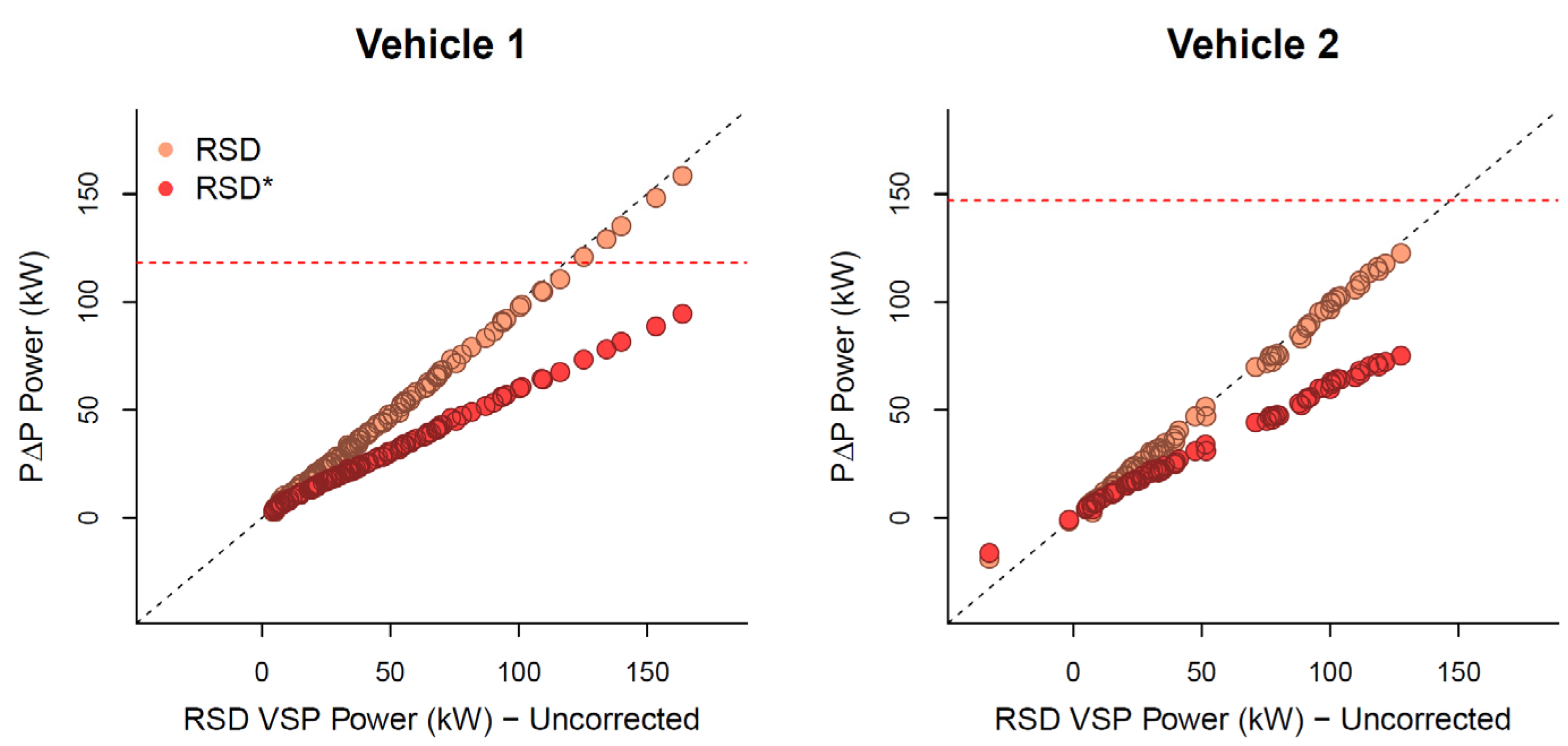
A comparison of VSP and and PΔP engine power shows similar results. Figure 8 compares VSP and PΔP engine power using RSD speed/acceleration gradient data. It also shows the corrected PΔP engine power using RSD acceleration values that were adjusted for time resolution.
Figure 8 shows that uncorrected VSP and PΔP engine power (denoted with RSD) are similar: data points are close to the dashed 45° line. Figure 8 shows that the uncorrected values exceed rated engine power (red dashed line) for vehicle 1. The PΔP engine power based on adjusted acceleration values achieves a realistic power range for both test vehicles and is used in further analysis.

2.10. RSD NO2 Emission Correction

Although NO2 measurement has recently become a feature of remote sensing [4], remote sensing studies have traditionally used RSDs that measure NO only, as is the case in this study. In contrast, dynamometer measurements relate to the sum of NO and NO2 (i.e., NOx, expressed as NO2 equivalents). Direct use of NO data from RSD would therefore result in an underestimation (bias) of RSD NOx emission rates.
Primary NO2-to-NOx ratios (fNO2) are critically dependent on type of emission control technology used. A review of the available evidence suggests that these ratios are significant for diesel E4 and E5 cars, varying between 25% to almost 80% in individual cases [19]. In addition, there is some evidence that larger (diesel) cars have higher NO2 emission rates [4], and that NO2-to-NOx ratios reduce as vehicles age [33]. There is limited information on the relationship between fNO2 and engine power. A few studies reported no discernible relationship between fNO2 and speed/acceleration or VSP [34,35,36]. The measured RSD NO concentration data was converted to NOx by computing NO/(1-fNO2), assuming an fNO2 value of 50% and 45% for the E4 and E5 test vehicle, respectively, based on a review of published data [19].

2.11. Humidity Correction

NOx emissions are a function of humidity, where an increase in ambient humidity lowers NOx emissions and vice versa (e.g., [37]). The RSD does not correct NO for humidity on NO emissions. Few remote sensing studies have actually measured humidity (e.g., [38]), or corrected remote sensing measurements for humidity [39].
In contrast, dynamometer NOx measurements report results in reference test conditions and use absolute humidity (g/kg dry air) to correct measured NOx within a specified temperature range (e.g., [40]). The aggregated humidity correction factor (KH factor) is reported for each dynamometer test. It varied between 1.10 and 1.15. Dividing the test results with the KH factor provides an estimate of uncorrected NOx emissions on the dynamometer. They are used in the next section.

3. Results and Discussion

3.1. Emission Measurement Results

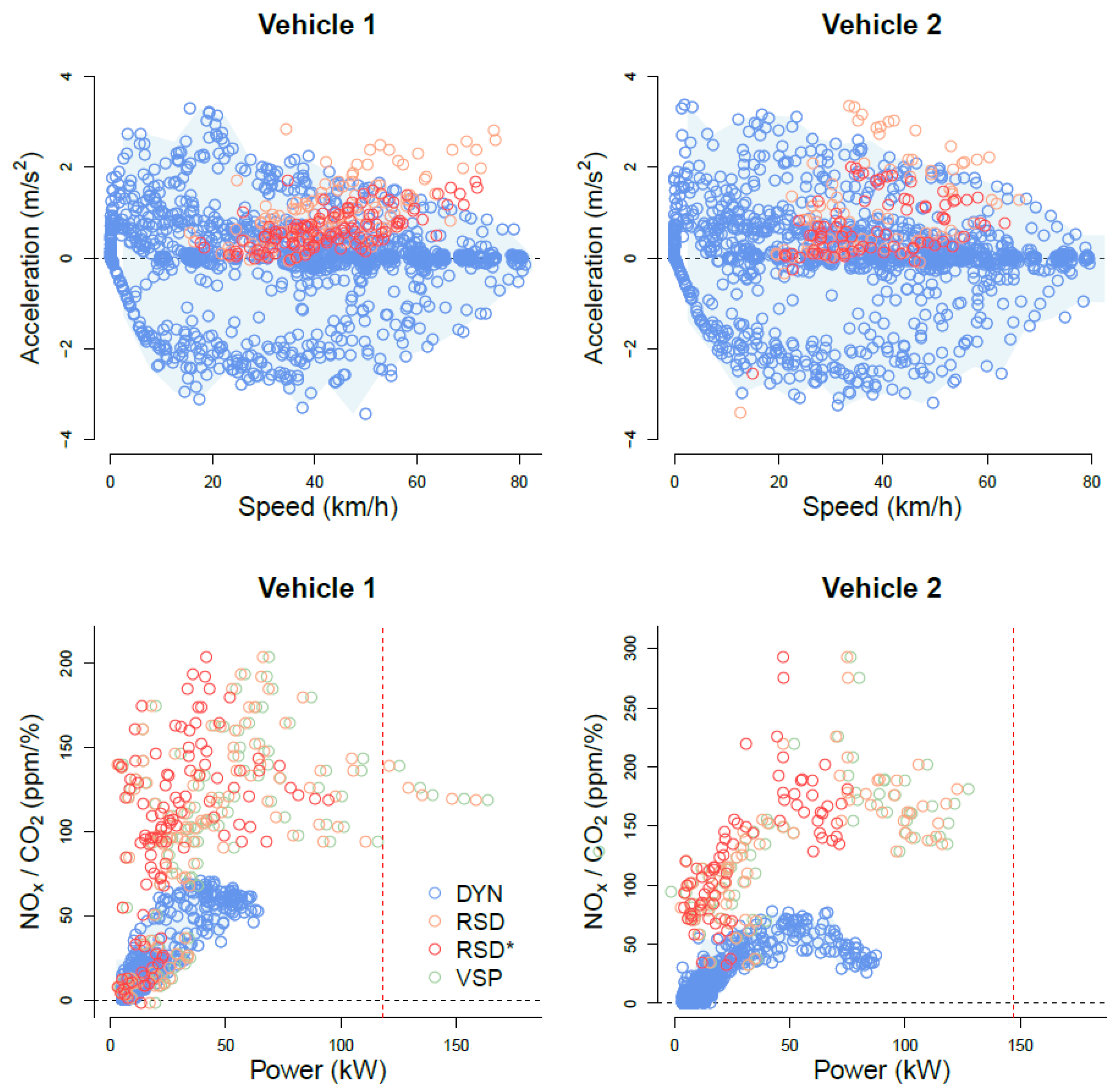
Figure 9 shows the combined results for the dynamometer (DYN) and RSD hot running emission measurements.
The scatter plots on the left show the speed/acceleration data for the dynamometer test and RSD measurements, either uncorrected (RSD) or corrected (RSD*). RSD* represents the corrected speed and acceleration values, as discussed in Section 2.8. The blue shaded area presents the dynamometer operational envelope. The shaded area was created by computing minimum and maximum acceleration values for incremental 5 km/h speed bins and applying cubic spline interpolation for missing data points.
It can be seen that the RSD operates in a small speed/acceleration area. The reason for this is that the RSD tends to automatically discard measurements in operating modes that generate relatively low emission levels (e.g., idling, deceleration, cruise). Corrected RSD speed/acceleration values fall within the operational area of the dynamometer test, which confirms that corrected values should be used in the equipment comparison.
The scatter plots on the right show the measured emissions and power data. The RSD reports concentration levels in the exhaust gas, i.e., CO2 (%), CO (%), HC (ppm) and NO (ppm), corrected for water and excess oxygen not used in the combustion process. However, the exhaust plume path length and the density of the observed plume are highly variable from vehicle to vehicle and are a function of the height of the vehicle’s exhaust pipe, wind direction and speed, and turbulence behind the vehicle, amongst other factors. The RSD can therefore only reliably measure ratios of CO, HC and NO to CO2. Emissions are therefore presented as measured NOx/CO2 ratios for both the dynamometer and RSD (ppm/%). Note that NOx and CO2 distance-based emission factors (dynamometer test) are presented in Table 1.
The two test vehicles were tested using the dedicated test cycle in two operating modes, air conditioning on and off. Figure 9 shows the emission measurement results for the two vehicles with air conditioning on. Figure 9 shows that a substantial power range is achieved, with the range increasing as speed increases. The maximum power for vehicle 1 and 2 is 64 kW (54% of rated engine power) and 87 kW (59% of rated engine power), respectively. The blue shaded area presents the dynamometer power-emission envelope. It is clear that uncorrected RSD power and VSP values are too high, significantly exceeding rated engine power in a few cases. The adjusted RSD power values fall within the dynamometer power-emission envelope.
Figure 9 shows that RSD NOx/CO2 ratios are significantly outside the range of observed NOx/CO2 ratios in the dynamometer tests. The ratio of maximum RSD to maximum DYN values is 2.9 for vehicle 1 (fNO2 = 0.50) and 3.8 for vehicle 2 (fNO2 = 0.45). However, a zero value for fNO2 for both vehicles brings the results in better agreement (Figure 10).
The discrepancy in measured NOx/CO2 ratios is likely caused by different factors, or a combination. First, it is unlikely that the fraction of NO2 in the exhaust (fNO2) is zero. Therefore, the dynamometer NOx sensor may not adequately measure NO2, thereby underestimating NOx. The Horiba MEXA 720 NOx analyser uses a zirconia oxide sensor, and although measuring NOx is specified, it may provide a limited response to NO2 [41].
Alternatively, the measured RSD NOx/CO2 ratios may be biased high, leading to overestimated ratios. As compared with the more controlled environment of dynamometer measurements, it is more challenging for remote sensing to measure vehicle emissions accurately. Exhaust emissions dilute rapidly, and the RSD needs to strike the right balance between measuring emissions from as many as possible vehicles and preventing incorrect or inaccurate measurements due to low signal-to-noise ratios.
RSD bias and associated offsets have been observed and discussed in the past (e.g., [16,42,43]). Optical misalignment and equipment vibration due to moving vehicles shaking the roadway or producing air pulses were reported as possible causes. Nevertheless, other studies have shown no significant bias issues with the low NO RSD emission measurements (e.g., [44]).
The correlation analysis in the next section assumes that the dynamometer has effectively measured NO and not NOx. As a consequence, for computational purposes, fNO2 is considered to be zero. The sensitivity of this assumption is verified later.

3.2. RSD–DYNO Correlation and Bias

To compare RSD and DYN emissions, emissions data is binned into 5 kW power bins and averaged (Figure 11). The relationship between power and NOx/CO2 ratio is hyperbolic with low NOx/CO2 ratios at low power levels and stable or reduced ratios at high power levels.
RSD data is naturally noisy and sufficiently large sample sizes are required to obtain significant results. This is reflected in the large confidence intervals in all power bins. The variability observed in the NOx/CO2 ratios measured by the dynamometer is significantly smaller. There are several data points where the confidence intervals for RSD and DYN do not overlap, in particular for vehicle 2, which indicates that there is generally a systematic difference in absolute measurements between the RSD and DYN. Figure 12 shows the mean observed NOx/CO2 ratios, including the 95% confidence intervals for the two emission measurement methods. The black dotted line represents the 45° line, whereas the red line represents a weighted least-squares regression (WLS) fit including 95% confidence intervals (red shaded polygon).
The weighted correlation coefficient rw was computed, where the effective variance in the binned remote sensing and dynamometer samples were used as weights [45,46].
Effective variance is a measure of the combined uncertainty when both the y- and x-values of an observation have measurement error. The standard variance (square of the standard error) of the y-value is added to the standard variance of the x-value multiplied by the slope, which is assumed to be 1. The weight for the observation is the inverse of the effective variance. Computation of rw for vehicle 1 and 2 showed a strong correlation between the dynamometer and RSD, i.e., +0.89 (vehicle 1) and +0.95 (vehicle 2).
Figure 12 also shows that there are significant positive intercepts for the fitted linear regression lines, i.e., vehicle 1 (21 ± 14 ppm/%) and vehicle 2 (30 ± 9 ppm/%) (mean ± 95% CI). This suggests that, in an absolute sense, low measured NO/CO2 ratios are not replicated in the remote sensing data. This bias is visible for both vehicles. For vehicle 1 the 95% confidence intervals are either close or overlap with the 45° line, which suggests that the differences may in fact not (always) be statistically significant, when considering the combined variability in the RSD and dynamometer data. It is unclear at this stage what causes the difference between the vehicles, but it could be related to different NO2 emission levels.
A second WLS model including ‘vehicle’ as a covariate is fitted to all data to examine this. The model has an intercept of 21 ppm/% (p < 0.01). The difference in intercepts between the two vehicles is 17 ppm/% and is statistically significant (p = 0.03). The interaction term was not significant (p = 0.91). This suggest that a constant bias correction between 21 and 30 ppm/% (e.g., 25 ppm/%) may be applicable to the RSD measurements, assuming that the DYNO measurements are more accurate.
Nevertheless, it is recommended that further dynamometer testing be conducted, preferably with an RSD and dynamometer facility that measure both NO and NO2. If a systematic and consistent bias is observed for multiple vehicles, a correction final function for RSD NO/CO2 ratios could be implemented, which could be either a constant offset value, or a linear function (offset, slope). It would be interesting to examine whether different vehicle types with different emission profiles (petrol car, diesel truck, motorcycle) will produce similar results. The evidence presented in this study may not be sufficient to develop robust correction functions for RSD4600 NO/CO2 ratio measurements, if indeed they are required pending further research. However, the analysis shows that the correlation between the RSD and dynamometer is strong, despite the high level of variability observed in the RSD measurements.

3.3. Sensitivity Analysis

A number of assumptions are made in this research. First, the RSD4600 does not measure NOx, but only NO. Therefore, an assumption is made regarding the proportion of direct NO2 in order to convert measured NO to NOx. Second, the use of 5 kW increments to define power bins appears to strike a reasonable balance between sample size and granularity but it is arbitrary. Third, the impact of including or excluding a humidity correction for NOx is of interest. Finally, given the widespread use of VSP in RSD studies, it is of interest to assess the impact of using VSP as reported by the RSD instead of simulated (PΔP) engine power. The sensitivity of the correlation between RSD and DYN to the assumptions used in this study have been quantified by varying the assumptions one-at-the-time (OAT) within a plausible range, while other settings are held constant [47]. The results are presented in Table 2.
Table 2 shows that the use of original RSD speed/acceleration or VSP data results in significant reductions in correlation. Correction of speed and acceleration (time resolution adjustment), and recalculation of VSP or other power estimation methods, is important. This is a relevant finding for emission factor development and model validation studies. The definition of power bin increments also has a substantial impact. An increase in the size of power bin increments may slightly improve the correlation, whereas a decrease in power bin increments can lead to a substantial reduction. This is due to the averaging effect of bin size on the total number of (mean) data points and the impact on ‘within-bin’ sample size, and consequently standard deviation, which are used as weights.
The plausible range in fNO2 values correction hardly impact on correlation. This is expected, as fNO2 adds a constant offset to the RSD and is assumed to be independent of engine power. The assumption of a constant fNO2 appears reasonable based on the available literature. Similarly, humidity hardly affects the correlation as it scales all emissions data using the KH factor. The use of different fNO2 values and humidity correction factors do impact on RSD bias correction. It is recommended that the correlation is further examined with an RSD that is capable of measuring both NO and NO2.

4. Conclusions

This study explores the correlation between a remote sensing device (RSD) and dynamometer testing. Two diesel cars were tested on the dynamometer and driven multiple times past the RSD in hot running conditions. A new dynamometer drive cycle was developed with the aim to replicate a range of typical driving behaviour that is expected to be observed in remote sensing studies, consisting of moderate to strong accelerations with different end speed points. A number of verification and correction steps were conducted for both the dynamometer and RSD data.
Dynamometer CO2 emissions were time aligned to ensure that good correlation between the emission rate and positive engine power was achieved. Additional power use by the air-conditioning systems was quantified through statistical analysis of dynamometer tests with air conditioning on and off. The humidity correction for NOx was reversed as RSD does not correct for humidity.
A time resolution adjustment factor was developed for RSD acceleration measurements after analysis of speed and acceleration data collected with automatic pneumatic loop detectors at two RSD sites. The adjustment factor creates more realistic acceleration and power estimates. The RSD NO emissions data is also converted to NOx by adding a plausible range of NO2 emissions.
Comparison of RSD and dynamometer data consistently shows a strong weighted correlation varying from +0.89 to +0.95, despite the high level of variability observed in the RSD measurements. This provides further evidence that relative changes in mean NO/CO2 ratios as measured with the RSD should provide robust emissions data for trend analysis. The correlation was not sensitive to humidity correction or assumptions regarding additional NO2 emissions. The correlation was sensitive to application of the acceleration adjustment factor and power bin definition.
In an absolute sense, discrepancies were observed where measured mean NOx/CO2 ratios with the RSD were significantly and systematically higher as compared with the dynamometer tests. To some extent, this may be caused by the dynamometer NOx sensor, which may not adequately measure NO2 emissions. Further testing is recommended for at least two test vehicles, preferably with an RSD and dynamometer facility that measure both NO and NO2.
If a systematic and consistent bias was then observed for multiple vehicles, a correction function for RSD NO/CO2 ratios could be considered. The evidence presented in this study does not provide sufficient data to develop robust correction functions for RSD4600 NO/CO2 ratio measurements, but the evidence suggests that a significant positive bias may be present in RSD data.

Supplementary Materials

The following are available online at https://www.mdpi.com/2073-4433/11/3/294/s1.

Author Contributions

Conceptualisation, R.S.; methodology, R.S. and D.K.; formal analysis, R.S.; investigation, R.S.; writing—original draft preparation, R.S.; writing, R.S., visualisation, R.S.; supervision, R.S.; project administration, R.S. All authors have read and agreed to the published version of the manuscript.

Funding

This research received no external funding.

Acknowledgments

The authors are grateful for the dynamometer testing conducted by Rod Chippendale of Brisbane City Council/Transport for Brisbane and additional information provided by Gareth Jones of the NSW Department of Planning, Industry and Environment. WA DER is acknowledged for kindly loaning the RSD equipment to the Department of Environment and Science (DES) for 6 months. Scott Bainbridge of the Western Australia Department of Water and Environmental Regulation (WA DWER, Australia), Barbara Downs and Abbie Brooke of Brisbane City Council (Australia), Elizabeth Somervell of NIWA (New Zealand) and Ray Wilson of the Department of Transport and Main Roads (DTMR, Australia) are acknowledged for their contributions to the on-road campaign.

Conflicts of Interest

The authors declare no conflict of interest.

References

  1. Caiazzo, F.; Ashok, A.; Waitz, I.A.; Yim, S.H.L.; Barrett, S.R.H. Air pollution and early deaths in the United States. Part I: Quantifying the impact of major sectors in 2005. Atmos. Environ. 2013, 79, 198–208. [Google Scholar] [CrossRef]
  2. Smit, R.; Brown, A.L.; Chan, Y.C. Do air pollution emissions and fuel consumption models for roadways include the effects of congestion in the roadway traffic flow? Environ. Model. Softw. 2008, 23, 1262–1270. [Google Scholar] [CrossRef]
  3. Smit, R.; Ntziachristos, L.; Boulter, P. Validation of road vehicle and traffic emission models—A review and meta-analysis. Atmos. Environ. 2010, 44, 2943–2953. [Google Scholar] [CrossRef]
  4. Sjödin, Å.; Borken-Kleefeld, J.; Carslaw, D.; Tate, J.; Alt, G.-M.; De la Fuente, J.; Bernard, Y. Comparing Emission Rates Derived from Remote Sensing with PEMS and Chassis Dynamometer Tests—CONOX Task 1 Report; Commissioned by Federal Office for the Environment: Switzerland; IVL Swedish Environmental Research Institute: Stockholm, Sweden, 2018; ISBN 978-91-88787-28-6. [Google Scholar]
  5. Smit, R.; Somervell, E. The Use of Remote Sensing to Enhance Motor Vehicle Emission Modelling in New Zealand; National Institute of Water & Atmospheric Research: Auckland, New Zealand, 2015. [Google Scholar]
  6. Smit, R.; Bluett, J. A new method to compare vehicle emissions measured by remote sensing and laboratory testing: High-emitters and potential implications for emission inventories. Sci. Total Environ. 2011, 409, 2626–2634. [Google Scholar] [CrossRef] [PubMed]
  7. Chen, Y.; Borken-Kleefeld, J. Real-Driving Emissions from Cars and Light Commercial Vehicles—Results from 13 Years Remote Sensing at Zurich/CH. Atmos. Environ. 2014, 88, 157–164. [Google Scholar] [CrossRef]
  8. Bernard, Y.; Tietge, U.; German, J.; Muncrief, R. Determination of Real-World Emissions from Passenger Vehicles Using Remote Sensing Data. The Real Urban Emissions Initiative (TRUE). 2018. Available online: https://www.trueinitiative.org/data/publications/determination-of-real-world-emissions-from-passenger-vehicles-using-remote-sensing-data (accessed on 15 August 2019).
  9. Smit, R.; Kingston, P.; Neale, D.W.; Brown, M.K.; Verran, B.; Nolan, T. Monitoring on-road air quality and measuring vehicle emissions with remote sensing in an urban area. Atmos. Environ. 2019, 218, 116978. [Google Scholar] [CrossRef]
  10. Bishop, G.A.; Starkey, J.R.; Ihlenfeldt, A.; Williams, W.J.; Stedman, D.H. IR long-path photometry: A remote sensing tool for automobile emissions. Anal. Chem. 1989, 61, 671–677. [Google Scholar] [CrossRef]
  11. Sjödin, Å.; Andréasson, K.; Wallin, M.; Lenner, M.; Wilhelmsson, H. Identification of high-emitting catalyst cars on the road by means of remote sensing. Int. J. Veh. Des. 1997, 18, 326–339. [Google Scholar]
  12. TRL. The Inspection of In-Use Cars in Order to Attain Minimum Emissions of Pollutants and Optimum Energy Efficiency—Remote Sensing; TRL: Crowthorne, UK, 1998. [Google Scholar]
  13. Pokharel, S.S.; Stedman, D.H.; Bishop, G.A. RSD Versus IM240 Fleet Average Correlations. In Proceedings of the 10th CRC On-Road Vehicle Emissions Workshop, San Diego, CA, USA, 27–29 March 2000. [Google Scholar]
  14. Yanowitz, J.; McCormick, R.L.; Graboski, M.S. In-use emissions from heavy-duty diesel vehicles. Environ. Sci. Technol. 2000, 34, 729–740. [Google Scholar] [CrossRef] [Green Version]
  15. Elder, S.; Graham, M.; Jones, K.; Raine, R. Vehicle Emissions Remote Sensing Campaign: Control Vehicle Study; UniServices Report 30793.001; University of Auckland: Auckland, New Zealand, 2011. [Google Scholar]
  16. Mazzoleni, C.; Moosmüller, H.; Kuhns, H.D.; Keislar, R.E.; Barber, P.W.; Nikolic, D.; Nussbaum, N.J.; Watson, J.G. Correlation between automotive CO, HC, NO, and PM emission factors from on-road remote sensing: Implications for Inspection and Maintenance Programs. Transp. Res. Part D Transp. Environ. 2004, 9, 477–496. [Google Scholar] [CrossRef]
  17. Rhys-Tyler, G.A.; Bell, M.C. Toward reconciling instantenous roadside measurements of light-duty vehicle exhaust emissions with type approval drive cycles. Environ. Sci. Technol. 2012, 46, 10532–10538. [Google Scholar] [CrossRef] [PubMed] [Green Version]
  18. Smit, R.; Kingston, P. Detecting cold start vehicles in the on-road fleet. Air Qual. Clim. Chang. 2019, 53, 22–26. [Google Scholar]
  19. Smit, R.; Kingston, P. Measuring on-road vehicle emissions with multiple instruments including remote sensing. Atmosphere 2019, 10, 516. [Google Scholar] [CrossRef] [Green Version]
  20. Smit, R. Development and performance of a new vehicle emissions and fuel consumption software (PΔP) with a high resolution in time and space. Atmos. Pollut. Res. 2013, 4, 336–345. [Google Scholar] [CrossRef] [Green Version]
  21. Smit, R. PΔP: A simulation tool for vehicle emissions and fuel consumption software with a high resolution in time and space. Veh. Technol. Eng. 2014, 2014, 17–21. [Google Scholar]
  22. Kent, J.H.; Allen, G.H.; Rule, G. A driving cycle for Sydney. Transp. Res. 1978, 12, 147–152. [Google Scholar] [CrossRef]
  23. Watson, H.C.; Milkins, E.E.; Braunsteins, J. The development of the Melbourne Peak Cycle. In Proceedings of the SAE-A/ARRB 2nd Conference on Traffic Energy and Emissions, Melbourne, Australia, 19–20 May 1982. [Google Scholar]
  24. DTRS. Comparative Vehicle Emissions Study; Commonwealth Department of Transport and Regional Services: Canberra, Australia, 2001; ISBN 0 642 45684 4. [Google Scholar]
  25. Orbital. NISE 2—Contract 2 Drive Cycle and Short Test Development; Orbital Australia Pty Ltd.: Balcatta, Australia, 2005. [Google Scholar]
  26. Wong, C.K.L.; Lo, T.S.; Wong, H.L.A.; Lam, K.L.; Frey, H.C.; Smit, R.; Hausberger, S.; Weller, K.; Ntziachristos, L. Microscale Vehicle Emission Modelling in Hong Kong. In Proceedings of the 23rd Transport and Air Pollution Conference 2019, Thessaloniki, Greece, 15–17 May 2019. [Google Scholar]
  27. Atjay, D.; Weilenmann, M.; Soltic, P. Towards accurate instantaneous emission models. Atmos. Environ. 2015, 39, 2443–2449. [Google Scholar]
  28. Efron, B. Bootstrap methods: Another look at the jackknife. Ann. Stat. 1979, 7, 1–26. [Google Scholar] [CrossRef]
  29. ESP. RSD4600 NextGen Operator’s Manual, 2nd ed.; Environmental Systems Products Holdings Inc.: Tucson, AZ, USA, 2006. [Google Scholar]
  30. Kuhns, H.D.; Mazzoleni, C.; Moosmuller, H.; Nikolic, D.; Keislar, R.E.; Barber, P.W.; Li, Z.; Etyemezian, V.; Watson, J.G. Remote sensing of PM, NO, CO and HC emission factors for on-road gasoline and diesel engine vehicles in Las Vegas, NV. Sci. Total Environ. 2004, 322, 123–137. [Google Scholar] [CrossRef]
  31. Smit, R.; Kingston, P.; Wainwright, D.; Tooker, R. A tunnel study to validate motor vehicle emission prediction software in Australia. Atmos. Environ. 2017, 151, 188–199. [Google Scholar] [CrossRef] [Green Version]
  32. Quaassdorff, C.; Smit, R.; Borge, R.; Hickman, M. Comparison of Microscale Traffic Emision Models for Urban Networks. In Proceedings of the CASANZ 2017 Conference, Brisbane, Australia, 15–18 October 2017. [Google Scholar]
  33. Carslaw, D.C.; Murrells, T.P.; Andersson, J.; Keenan, M. Have vehicle emissions of primary NO2 peaked? Faraday Discuss 2016, 189, 439–454. [Google Scholar] [CrossRef] [PubMed]
  34. Jimenez-Palacios, J.C. Understanding and Quantifying Motor Vehicle Emissions with Vehicle Specific Power and TILDAS Remote Sensing. Ph.D. Thesis, Department of Mechanical Engineering, Massachusetts Institute of Technology, Cambridge, MA, USA, February 1999. [Google Scholar]
  35. Carlsaw, D.C.; Rhys-Tyler, G. Remote Sensing of NO2 Exhaust Emissions from Road Vehicles; DEFRA Project Reference: 332c2011 (City of London Corporation); 334c2011 (London Borough of Ealing); City of London Corporation: London, UK, 16 July 2013. [Google Scholar]
  36. Moody, A.; Tate, J. In service CO2 and NOx emissions of Euro 6/VI cars, light- and heavy-duty goods vehicles in real London driving: Taking the road into the laboratory. J. Earth Sci. Geotech. Eng. 2017, 7, 51–62. [Google Scholar]
  37. Pekula, N.; Kuritz, B.; Hearne, J.; Marchese, A.J.; Hesketh, R.P. The Effect of Ambient Temperature, Humidity, and Engine Speed on Idling Emissions from Heavy-Duty Diesel Trucks. SAE Tech. Pap. Ser. 2003, 112, 148–158. [Google Scholar]
  38. Burgard, D.A.; Bishop, G.A.; Stedman, D.H.; Gessner, V.H.; Daeschlein, C. Remote sensing of in-use heavy-duty diesel trucks. Environ. Sci. Technol. 2006, 40, 6938–6942. [Google Scholar] [CrossRef] [PubMed]
  39. Bishop, G.A.; Morris, J.A.; Stedman, D.H.; Cohen, L.H.; Countess, R.J.; Countess, S.J.; Maly, P.; Scherer, S. The effect of altitude on heavy-duty diesel truck on-road emissions. Environ. Sci. Technol. 2001, 35, 1574–1578. [Google Scholar] [CrossRef]
  40. Lindhjem, C.; Chan, L.; Pollack, A.; Kite, C. Applying Humidity and Temperature Corrections to on and Off-Road Mobile Source Emissions. In Proceedings of the EPA 13th International Emission Inventory Conference: Working for Clean Air in Clearwater, Clearwater, FL, USA, 8–10 June 2004. [Google Scholar]
  41. Horiba, Introduction to HORIBA “On Board” System for PEMS Project. December 2014. Available online: https://circabc.europa.eu/webdav/CircaBC/GROW/pems/Library/pems_meetings_2004-2005/brussels_13-14th/P2_HORIBA_OBS_PEMS_13-12-04.pdf (accessed on 15 August 2019).
  42. Stephens, R.D.; Cadle, S.H. Remote sensing measurements of carbon monoxide emissions from on-road vehicles. J. Air Waste Manag. Assoc. 1991, 41, 39–46. [Google Scholar] [CrossRef]
  43. Bishop, G.A.; Stedman, D.H. Measuring the emissions of passing cars. Acc. Chem. Res. 1996, 29, 489–495. [Google Scholar] [CrossRef]
  44. Kraan, T.C.; Baarbe, H.L.; Eijk, A.R.A.; Stelwagen, U.; Vonk, W.A. Consistency Tests of Remote Sensing for Vehicle Exhaust Emissions. In Proceedings of the 19th Transport and Air Pollution Conference, Thessaloniki, Greece, 26–27 November 2012. [Google Scholar]
  45. Tellinghuisen, J. Least-squares analysis of data with uncertainty in X and Y: A Monte Carlo methods comparison. Chemom. Intell. Lab. Syst. 2010, 103, 160–169. [Google Scholar] [CrossRef]
  46. Revelle, W. Psych: Procedures for Personality and Psychological Research, version 1.8.12; North Western University: Evanston, IL, USA, 2018. [Google Scholar]
  47. Saltelli, A.; Chan, K.; Scott, E.M. Sensitivity Analysis; John Wiley & Sons Ltd.: Chichester, UK, 2000. [Google Scholar]
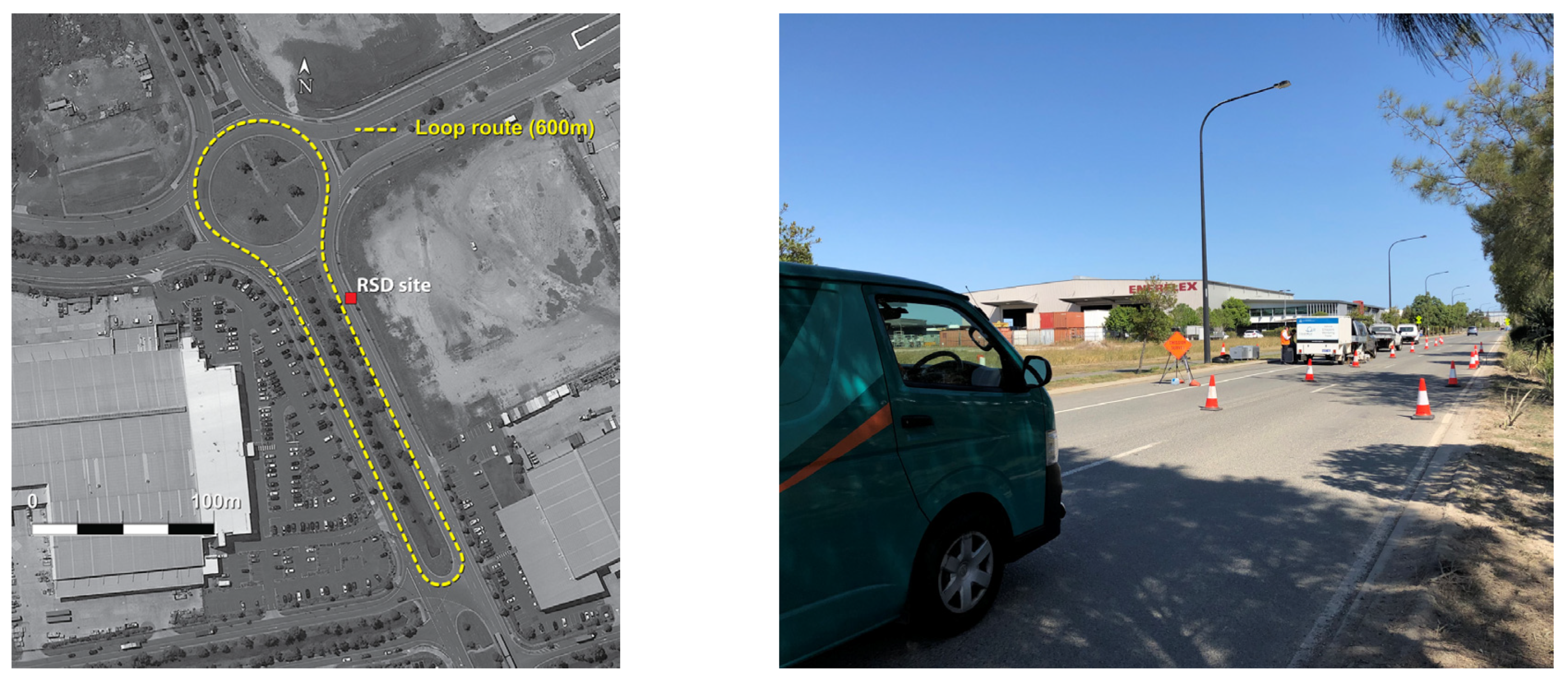
Figure 1. Remote sensing device (RSD) test route at the commercial RSD site.
Atmosphere 11 00294 g001
Figure 2. Transient vehicle dynamometer setup.
Atmosphere 11 00294 g002
Figure 3. Simulation of test vehicles over Australian drive cycles. Red lines in left side plots show the binned (5 km/h bins) maximum acceleration values, red lines in centre plots show zero speed, and red lines in right side plots show rated engine power.
Atmosphere 11 00294 g003
Figure 4. Developing speed/acceleration functions from real-world drive cycles; red, green and blue solid dot points show the binned (5 km/h bins) maximum, median and minimum acceleration values; the corresponding coloured lines show the sigmoid models fitted to these points.
Atmosphere 11 00294 g004
Figure 5. Drive cycle for RSD–dynamometer comparison.
Atmosphere 11 00294 g005
Figure 6. Measured CO2 and dynamometer power with air conditioning on and off.
Atmosphere 11 00294 g006
Figure 7. Speed and acceleration data measured with two devices at the urban and freeway test sites.
Atmosphere 11 00294 g007
Figure 8. Estimates of engine power using RSD data for the two test vehicles (RSD = original measured acceleration, RSD* = adjusted acceleration).
Atmosphere 11 00294 g008
Figure 9. Dynamometer and RSD speed, power and hot running emissions data (rated engine power is dashed red line).
Atmosphere 11 00294 g009
Figure 10. Dynamometer and RSD speed, power and hot running emissions data (assuming fNO2 is zero).
Atmosphere 11 00294 g010
Figure 11. Mean hot running emission ratios versus power, including 95% confidence intervals. The open dot points represent data with a single observation.
Atmosphere 11 00294 g011
Figure 12. RSD and DYN mean hot running emission ratios, including 95% confidence interval.
Atmosphere 11 00294 g012
Table 1. Test vehicle specifications and selected dynamometer test results.
Design Parameter/Test VariableVehicle 1Vehicle 2
Model/MakeFord RangerFord Ranger
Model year20162017
Emission standardEuro 4Euro 5
Engine capacity (litres)2.23.2
Emission control technologyDOC, EGRDOC, EGR, DPF
Tare weight (kg)19382135
Test weight (kg)22402700
Vehicle loading (%)60%53%
Gross vehicle weight (kg)32003200
Rated engine power (kW)118147
CdA (m2) *0.720.70
RSD test cycle average speed (km/h)3029
RSD test cycle average NOx emission factor (g/km)1.11.3
RSD test cycle average CO2 emission factor (g/km)458506
* CdA is the product of the aerodynamic drag coefficient and the frontal area. DOC, diesel oxidation catalyst; EGR, Exhaust Gas Recirculation; DPF, diesel particulate filter.
Table 2. Weighted correlation coefficients for different scenarios.
Scenario DescriptionScenario DefinitionVehicle 1Vehicle 2
Base casefNO2 (Veh 1) = 0, fNO2 (Veh 2) = 00.890.95
RSD acceleration = adjusted
RSD power definition = PΔP engine power
Power bin increment = 5 kW
Humidity correction = excluded
Original RSD Base case, but RSD acceleration = original0.830.62
Original RSD VSPBase case, but RSD VSP = original0.730.64
Minimum power binBase case, but Power bin increment = 1 kW0.390.85
Maximum power binBase case, but Power bin increment = 10 kW0.930.94
Minimum fNO2Base case, but fNO2 (Vehicle 1/2) = 0.28/0.250.880.95
Maximum fNO2Base case, but fNO2 (Vehicle 1/2) = 0.77/0.700.880.94
Humidity correctionBase case, but humidity correction applied0.890.94