Probabilistic Forecast of Low Level Wind Shear of Gimpo, Gimhae, Incheon and Jeju International Airports Using Ensemble Model Output Statistics

Abstract

Wind shear can occur at all flight levels; however, it is particularly dangerous at low levels, from the ground up to approximately 2000 feet. If this phenomenon can occur during the take-off and landing of an aircraft, it may interfere with the normal altitude change of the aircraft, causing delay and cancellation of the aircraft, as well as economic damage. In this paper, to estimate the probabilistic forecasts of low-level wind shear at Gimpo, Gimhae, Incheon and Jeju International Airports, an Ensemble Model Output Statistics (EMOS) model based on a left-truncated normal distribution with a cutoff zero was applied. Observations were obtained from Gimpo, Gimhae, Incheon and Jeju International Airports and 13 ensemble member forecasts generated from the Limited-Area Ensemble Prediction System (LENS), for the period December 2018 to February 2020. Prior to applying to EMOS models, statistical consistency was analyzed by using a rank histogram and kernel density estimation to identify the uniformity of ensembles with corresponding observations. Performances were evaluated by mean absolute error, continuous ranked probability score and probability integral transform. The results showed that probabilistic forecasts obtained from the EMOS model exhibited better prediction skills when compared to the raw ensembles.

1. Introduction

Due to dangerous weather events related to wind, such as wind storm, wind shear and turbulence, users’ complaints and economic damage caused by flight delays and cancellations are continuously occurring [1]. In order to reduce the damage, it is necessary to develop technologies to improve the accuracy of forecasts and warnings for dangerous weather events occurring at airports.

The Low-Level Wind Shear (LLWS) is defined as a vector difference that is composed of wind speed and wind direction between two wind velocities in the lower levels below 2000 feet of the surface. It signifies vertical wind shear that is determined by means of two points at different heights in this study. The sudden LLWS can severely impact airplanes, especially within 2000 feet above ground level because of limited vertical airspace for recovery (ICAO, 2005). Therefore, preparing for the LLWS through wind shear forecasts at lower levels is very important for safe operations of aircrafts.

Ensemble forecasts have the features and advantages that can provide a variety of information, such as forecast range, diversity, probability distribution and uncertainty in both the data and model. Therefore, the probabilistic information from the ensemble forecasts may help to improve the safeness of aircraft operations. The Met office has developed an ensemble forecast system by using the Met Office Global and Regional Ensemble Prediction System (MOGREPS) to produce a probabilistic indicator of wind shear and convectively induced turbulence [2]. The National Centers for Environmental Prediction (NCEP) of National Oceanic and Atmospheric Administration (NOAA) has been making efforts to provide probabilistic information of aviation-related ensemble products, including LLWS, using the Short Range Ensemble Forecast (SREF) system [3]. Moreover, the ensemble forecast of LLWS has tried to verify and evaluate by using the NCEP forecast verification system [4]. Furthermore, the NCEP Very Short Range Ensemble Forecast (VSREF) was developed to forecast aviation-weather-related products, including LLWS, every 1 h [5]. Recently, Lee et al. [6] conducted a reliability analysis and evaluation to verify LLWS ensemble member forecasts and local data assimilation and prediction system analyses data based on grid points over the Jeju area.

Estimating low-level wind shear by using ensemble member forecasts generated from Limited-Area Ensemble Prediction System (LENS) cannot guarantee accuracy of predictions because of the inherent bias and variability within the system itself [7]. Therefore, various statistical postprocessing techniques have been applied to calibrate the bias and variability inherent in the ensemble models [8,9,10]. Among these statistical postprocessing methods, one of the most popular methods is a probabilistic forecast that can provide probability information by estimating a fully probability density function for the future weather event [11,12,13,14,15,16].

In this study, Ensemble Model Output Statistics (EMOS) was applied to low-level wind shear in Gimpo, Gimhae, Incheon and Jeju International Airports to provide detailed weather information and corresponding ensemble forecasts required to generate probabilistic forecasts and to compare the prediction skills. The EMOS model for ensemble forecasts was suggested by Gneiting et al. (2005). They used a single normal distribution, where the mean is an affine function of the ensemble members, and the variance is an affine function of the ensemble variable. Since only non-negative values and a skewed distribution are allowed for low-level wind shear, we used a left-truncated normal distribution with a cutoff at zero for low-level wind shear. Prior to applying EMOS model, statistical consistency was analyzed to evaluate the reliability of the LLWS ensembles. Moreover, the prediction skills of the probabilistic forecasts were assessed in terms of mean absolute error (MAE), continuous ranked probability score (CRPS) and probability integral transform (PIT).

The rest of paper is organized as follows: the datasets used for the analysis and analytic method are briefly described in Section 2 and Section 3, respectively. The reliability analysis of the raw ensembles and its corresponding analysis, prediction skills of ensemble forecasts and probability that occur at a specific event through the estimation of the predictive probability density function are presented in Section 4. Finally, conclusions are given in Section 5.

2. Data

For this study, the high-resolution Limited-Area Ensemble Prediction System (LENS) is used based on the Korea Meteorological Administration (KMA) Unified Model (UM) to conduct probability forecasting of LLWS. The LENS was developed and operational in 2015 and considered of a control member with 12 perturbed members. It has horizontal resolution of 2.2 km with a rotated equatorial latitude–longitude coordinate system and 70 vertical levels with a top at approximately 40 km. The global Ensemble Prediction System (EPS) of the KMA uses Ensemble Transform Kalman Filter (ETKF) to produce 24 members, including the control member [17,18,19]. Among these global ensemble members, 12 perturbed members are randomly selected from global ensemble members and used as the initial and boundary conditions for LENS [20]. The LENS ran twice a day at 00 UTC and 12 UTC out to a lead time of 72 h (3 days) over the Korea Peninsula [16].

The LLWS is defined as the difference between two winds at different levels and assumed as linear wind shear at low level. Therefore, the ensemble forecasts of wind components at each grid point are interpolated at interval of 100 feet from 100 to 2000 feet. The LLWS ensemble forecasts are calculated at 19 levels.

The definition of LLWS is as follows:

$$\mathrm{LLWS}=\sqrt{{\left(\frac{\partial u}{\partial z}\right)}^2+{\left(\frac{\partial v}{\partial z}\right)}^2}$$

(1)

where ∂z is interval of vertical level which means 100 feet. The u and v are zonal and meridional component of wind, respectively. The unit of LLWS is knots/100 feet.

The Aircraft Meteorological Data Relay (AMDAR) data include wind and temperature from surface to upper-level corresponding to the location of the aircraft [21]. Therefore, the LLWS is available to obtain by using the wind data of AMDAR. For this study, LLWS of AMDAR data obtained from the domestic aircraft for four main international airports (Gimhae, Gimpo, Incheon, Jeju) in Republic of Korea were used as observed data to verify the probability forecasts of LLWS. The data are calculated in the same way as LLWS forecasts below 2000 feet during the aircraft landing.

For this study, the probability forecasts of LLWS were produced by using the ensemble forecast data of LENS from 3 to 24 h (1 day) and analyzed with LLWS of AMDAR at each airport, from December 2018 to February 2020. Prior to analysis, the missing values of the ensemble forecasts and their corresponding observations for the entire period were checked, and if either was absent, both were removed from the datasets.

First, the characteristics of the empirical distribution of ensemble member forecasts and its corresponding observations were examined at Gimpo, Gimhae, Incheon and Jeju International Airports for the entire period. Moreover, the reliability analysis for each international airport was conducted by using a rank histogram and reliability index to identify the statistical consistency of ensemble member forecasts and corresponding observations.

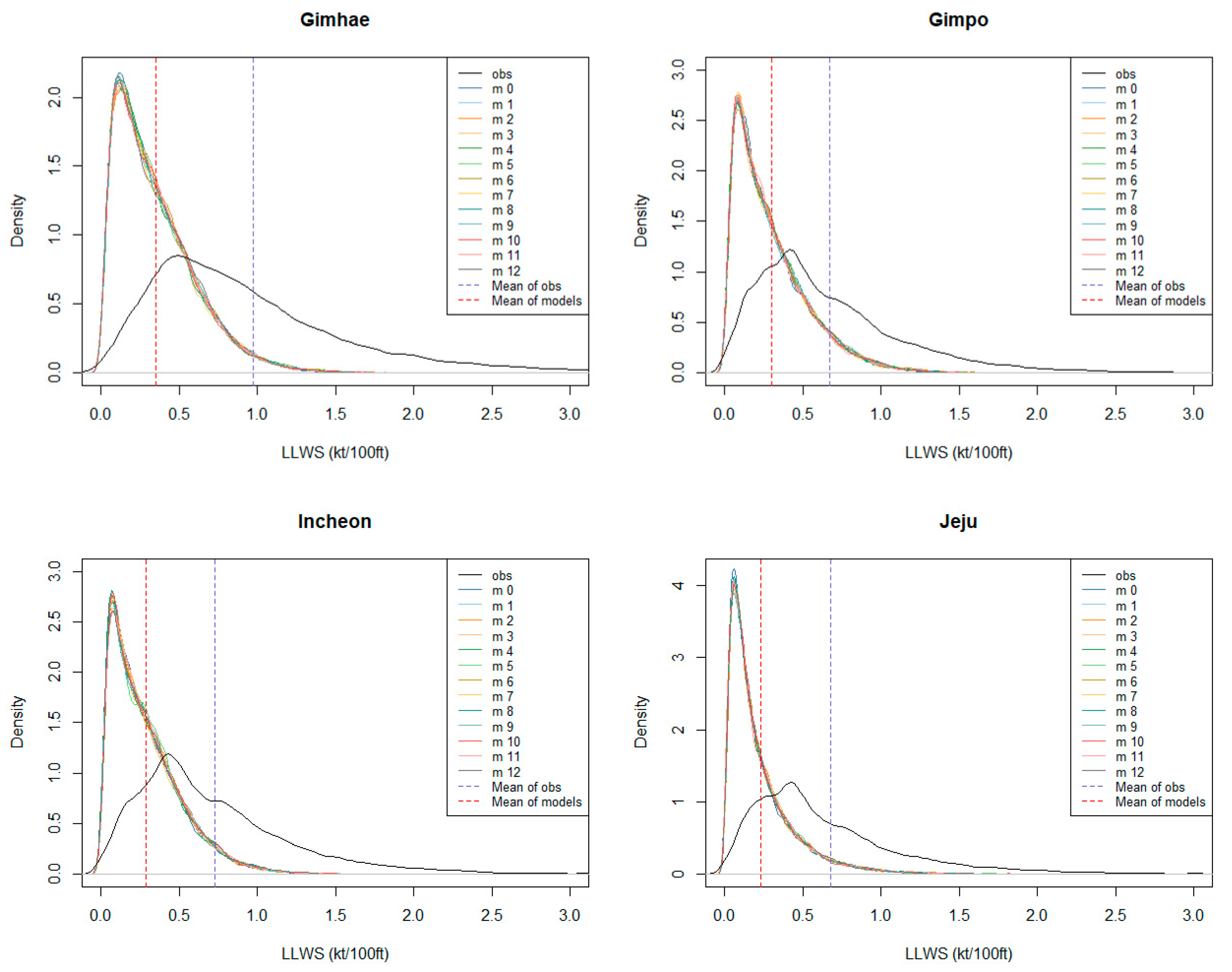
In Figure 1, the distributions of the ensembles and observations were estimated by using a kernel density estimation technique to examine the distributional characteristics of LLWS for each airport. The solid black line denotes the distribution of the observed LLWS, and the remaining colored lines denote the distributions of the 13 ensemble member forecasts, respectively. The red dotted line represents the average of the ensembles, and the blue dotted line represents the mean of observations.

For Gimhae airport, the distributions among the ensemble member forecasts are very similar. On the other hand, it can be seen that the distribution of the ensembles has relatively small variability compared to the observed LLWS distribution. It is also shown that the ensembles are underestimated on average compared to the corresponding observations. This implies that the ensemble member forecasts have negative biases on average compared to observations and have under-dispersion. It also has a value greater than 0, due to the nature of wind, and has asymmetric and left-skewed distribution. In the case of other airports, there is a slight difference in the distribution, but it shows the same pattern as indicated in the Gimhae airport, which shows underestimation and under-dispersion.

A rank histogram (RH) [22,23] was used to assess the reliability of LLWS of ensemble forecasts and their corresponding observations at each airport. The RH is a very useful visual tool for evaluating the reliability of ensembles and for identifying errors related to their mean and spread.

The RH for 13 ensembles and the corresponding observed LLWS are presented in Figure 2. In general, the RHs show similar trends and dispersions for each airport. For all airports, RHs with high counts near the right extreme and low frequency counts near the left extreme represents asymmetric errors in the data of the ensembles, implying ensemble forecasts have a strong negative bias, which indicates an underestimation. Moreover, RH has a U-shaped pattern, indicating a weak under-dispersion.

The reliability index [24] was used to quantify the deviation of the rank histogram from uniformity. If the ensemble forecasts and observations were obtained from the same distribution, the reliability index should be zero. The reliability index for each airport in Figure 2 is listed in

Table 1. Reliability index for airports.

	Gimhae	Gimpo	Incheon	Jeju
Reliability Index	1.2245	1.0418	1.1680	1.2322

, and their values show they are far from uniformity.

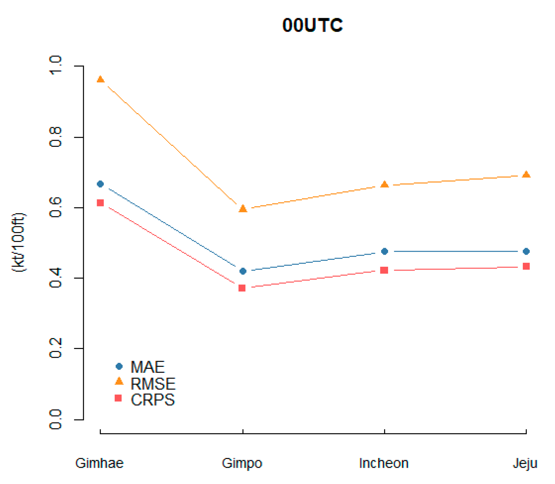
The prediction performance was analyzed in terms of mean absolute error (MAE), root mean square error (RMSE) and continuous ranked probability score (CRPS), using the ensemble mean obtained from the ensemble member forecasts. The prediction skills of the ensemble mean for each airport are given in Figure 3 and

Table 2. MAE, RMSE of ensemble mean and CRPS of ensemble forecasts.

Airport (00UTC)	Ensemble Mean		Ensemble
	MAE	RMSE	CRPS
Gimhae	0.668	0.961	0.612
Gimpo	0.420	0.594	0.372
Incheon	0.475	0.662	0.422
Jeju	0.477	0.691	0.433

. It can be seen that the performance of the prediction error in Gimpo airport is better than that of the other airports; the Gimhae airport consistently shows the worst performance. The prediction error for the ensemble mean was obtained to be small in terms of three measurements, because both ensembles and observations were small. Even if these values are small, they cannot be said to have good prediction performance.

3. Methodology

As 13 ensemble member forecasts simulated from LENS have negative bias and weak under-dispersion, the statistical postprocessing method was applied to calibrate them. Among the statistical postprocessing techniques, the most widely applied method is a probabilistic forecast that estimates a fully probability density function for future weather quantity and provides probability information by using it.

There are various methods for probabilistic prediction techniques, but among them, the Ensemble Model Output Statistics (EMOS) model was applied in order to take into account the LLWS. Since only non-negative values and a skewed distribution are allowed for LLWS, we use a left-truncated normal distribution with a cutoff zero for LLWS. Let a random variable, $\mathrm{y}$, have a normal distribution left-truncated at zero with location, $\mathsf{\mu }$, and standard deviation, $\mathsf{\sigma }$, denoted by $\mathrm{Y}~\mathrm{TN}\left(\mathsf{\mu },{\sigma }^2\right),$

$$\mathrm{h}\left(\mathrm{y}|\mathsf{\mu },{\sigma }^2\right)=\frac{1}{\sqrt{2\pi {\sigma }^2}}\frac{1}{\mathrm{\Phi }\left(\frac{\mu }{\sigma }\right)}exp\left(-\frac{{\left(y-\mu \right)}^2}{2{\sigma }^2}\right), y>0$$

(2)

where $\mathrm{\Phi }(·)$ is the cumulative distribution function (cdf) of the standard normal distribution.

Let $f_k$ denote the $k^{\mathrm{th}}$ ensemble member forecast of LLWS and $S_i^2=1/\left(M-1\right){\sum }_{j=1}^M{(f_{ij}-\overline{f_i})}^2$ denote the $i^{\mathrm{th}}$ sample variance of ensemble member forecasts. Gneiting et al. [9] suggested a heterogeneous regression model in which the variance of the error term is a linear function of the ensemble variance as follows:

$$\mathrm{Var}\left({\epsilon }_i\right)=c+d{S}_I^2$$

(3)

where $c$ and $d$ are positive variance coefficients. Variance coefficients $c$ and $d$ can be analyzed in terms of ensemble spread and skill of the ensemble mean. Under the same conditions, a spread-skill correlation is strong if the $d$ is high. On the contrary, when the spread and skill are independent of each other, it is estimated that d is low enough to be ignored.

The predictive distribution of EMOS model for LLWS is as follows:

$$\begin{array}{l}\mathrm{h}\left({\mathrm{y}}_i|b_0+b_1{f}_{i,1}+\cdots +b_{13}{f}_{i,13},\mathrm{c}+\mathrm{d}{S}_i^2\right)\\ \hspace{1em}\hspace{1em}\hspace{1em}\hspace{1em}\hspace{1em}\hspace{1em}\hspace{1em}=\frac{1}{\sqrt{2\pi \left(c+d{S}_i^2\right)}}\frac{1}{\mathrm{\Phi }\left(\frac{\mu b_0+b_1{f}_{i,1}+\cdots +b_{13}{f}_{i,13}}{\sqrt{\mathrm{c}+\mathrm{d}{S}_i^2}}\right)}exp\left(-\frac{{\left(y-b_0-b_1{f}_{i,1}-\cdots -b_{13}{f}_{i,13}\right)}^2}{2\left(\mathrm{c}+\mathrm{d}{S}_i^2\right)}\right), y>0\end{array}$$

(4)

where $b_k$ denotes the regression coefficients of ensemble member forecasts, and c and d are the nonnegative variance coefficients.

The CRPS (Continuous Ranked Probability Score) [23,25] estimation is used to estimate the regression coefficients and variance coefficients based on the training datasets. The CRPS is defined as follows.

$$\mathrm{crps}\left(\mathrm{F},\mathrm{y}\right)={{\displaystyle \int }}_{-\infty }^{\infty }{\left[F\left(t\right)-H\left(t-y\right)\right]}^{2}dt$$

(5)

where $\mathrm{H}(·)$ is the Heaviside function, which is 1 if the argument is positive and zero otherwise. Thorarinsdottir and Gneiting [11] showed the closed form of CRPS in Equation (5) for the truncated normal distribution, $\mathrm{TN}\left(\mathsf{\mu },{\sigma }^2\right)$. In this case, we tried to estimate regression and variance coefficients that minimize the CRPS:

$$mi{n}_{b_0,b_1,\cdots ,b_{13}, c, d}\frac{1}{n}{\sum }_{i=1}^n\sqrt{c+d{S}_i^2}\mathrm{\Phi }{\left(v_i\right)}^{-2}\left[Z_i\mathrm{\Phi }\left(Z_i\right)\left\{2\mathrm{\Phi }\left(Z_i\right)+\mathrm{\Phi }\left(v_i\right)-2\right\}+2\varphi \left(Z_i\right)\mathrm{\Phi }\left(v_i\right)-\frac{1}{\sqrt{\pi }}\mathrm{\Phi }\left(\sqrt{2}{v}_i\right)\right]$$

(6)

where $v_i=\frac{b_0-b_1{f}_{i,1}+\cdots +b_{13}{f}_{i,13}}{\sqrt{c+d{S}_i^2}}$, $Z_i=\frac{y_i-b_0-b_1{f}_{i,1}+\cdots +b_{13}{f}_{i,13}}{\sqrt{c+d{S}_i^2}}$, and $\varphi (·)\mathrm{and}\mathrm{\Phi }(·)$ are the probability density function and the cumulative distribution function of the standard normal distribution, respectively.

Since the estimated regression coefficients can be said to reflect general prediction skill on ensemble members compared with other ensemble members during the training period, they were estimated to be non-negative regression coefficients. For the computation optimization, we used the Broyden–Fletcher–Goldfarb–Shanno algorithm as implemented in R [26].

4. Results

A training period should be chosen to estimate the regression and variance coefficients of homogeneous and non-homogeneous regression (or EMOS) models, respectively. Since the wind characteristics are affected by the season, we tried to predict the low-level wind shear for each season to take this into account. The training and test periods for each season are given in

Table 3. Training and test periods for each season.

2018	2019												2020
12	1	2	3	4	5	6	7	8	9	10	11	12	1	2
train		test	train		test	train		test	train		test	train		test
2018/2019 DJF			2019 MAM			2019 JJA			2019 SON			2019/2020 DJF

. In order to estimate the regression and variance coefficients from the predictive probability density function for each season, we set two months as the training period, and the remaining is used as the test period.

Prior to applying the probabilistic forecast model, reliability (or statistical consistency) of the ensemble forecasts was examined by using rank histogram and reliability index to identify the ensemble and the corresponding observations. If the rank histogram is consistent with a uniform distribution, then we may conclude that the observation and the ensemble forecasts could have derived from the same distribution.

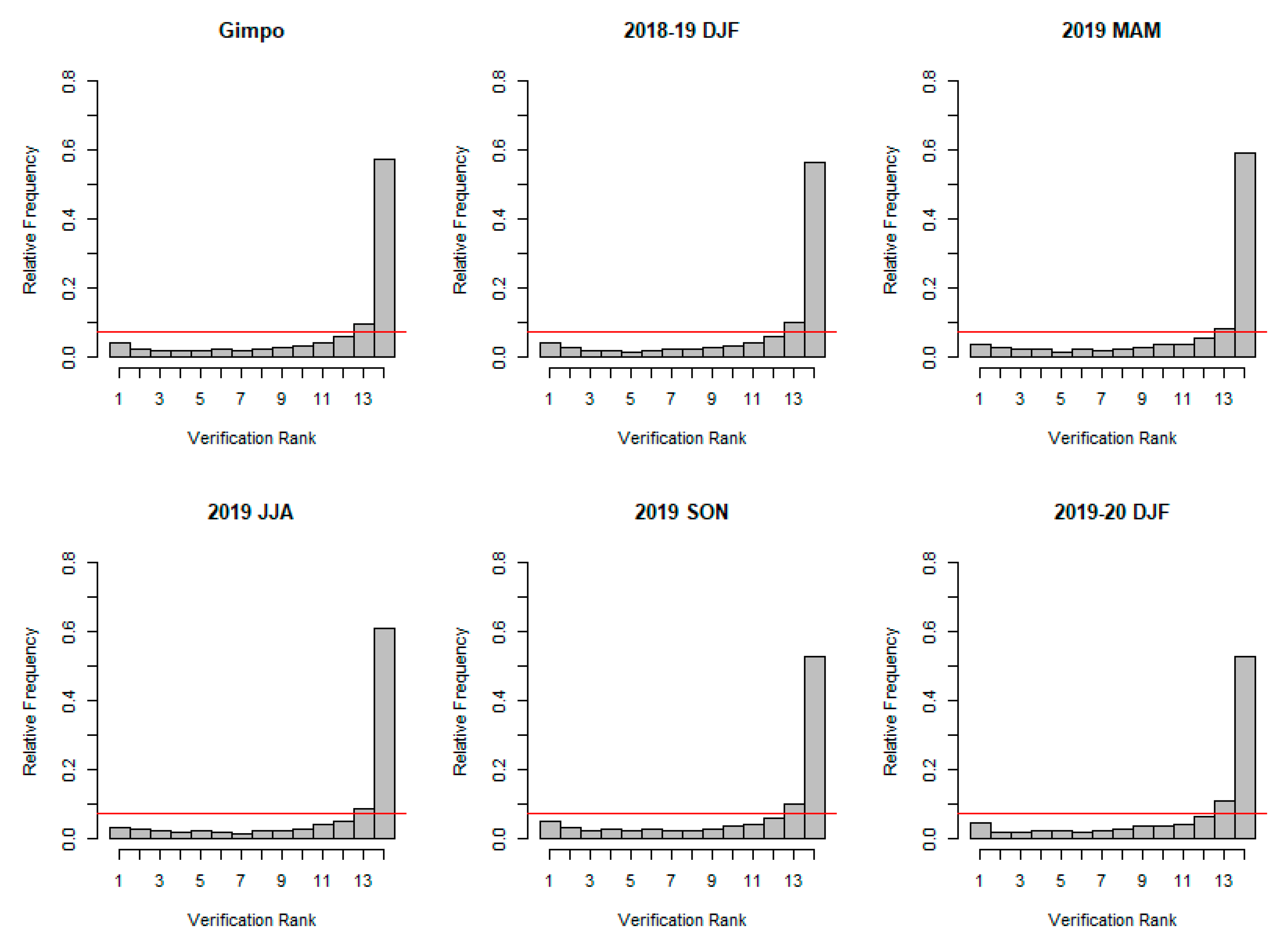
The verification rank histogram and reliability index by season at Gimhae airport are given in Figure 4 and

Table 4. Reliability index for Gimhae airport.

Gimhae	Entire Period	2018–19 DJF	2019 MAM	2019 JJA	2019 SON	2019–20 DJF
Reliability Index	1.2245	1.1335	1.2642	1.3649	1.1718	1.1658

, respectively. In Figure 4, the first figure is the rank histogram for the entire period of Gimhae airport, and the remaining five figures are the rank histograms for each season. It can be seen that the rank histogram for entire period and rank histogram for each season have similar patterns. The rank histogram shows that the ensemble forecast has a consistent negative bias, which implies an underestimation, such that the ensembles are generally less than observations. Moreover, the rank histogram is U-shaped, thus verifying that ensemble forecasts have under-dispersion, which indicates that the dispersion of ensembles is less than that of the corresponding observations.

The reliability index is used to quantify the deviation of the rank histogram from uniformity. The reliability index is defined by the average of the absolute difference of the observed relative frequency and true relative frequency in each bin. If the ensemble forecasts and the corresponding observations may have the same distribution, the reliability index should be zero. The reliability indexes for Figure 4 are presented in Table 4. From Table 4, it can be seen that they are almost the same values, and it is far from uniformity. Therefore, it would need to require statistical post-processing to calibrate the ensembles.

The verification rank histogram and reliability index by season at Gimpo airport are given in Figure 5 and

Table 5. Reliability index for Gimpo airport.

Gimpo	Entire Period	2018–19 DJF	2019 MAM	2019 JJA	2019 SON	2019–20 DJF
Reliability Index	1.0418	1.0386	1.0585	1.0971	0.9700	0.9811

, respectively.

The verification rank histogram and reliability index by season at Incheon airport are given in Figure 6 and

Table 6. Reliability index for Incheon airport.

Incheon	Entire Period	2018–19 DJF	2019 MAM	2019 JJA	2019 SON	2019–20 DJF
Reliability Index	1.1680	1.2167	1.1266	1.1472	1.1836	1.1690

, respectively.

The verification rank histogram and reliability index by season at Jeju airport are given in Figure 7 and

Table 7. Reliability index for Jeju airport.

Jeju	Entire Period	2018–19 DJF	2019 MAM	2019 JJA	2019 SON	2019–20 DJF
Reliability Index	1.2322	1.3720	1.1487	1.1014	1.2787	1.2940

, respectively. The rank histogram and reliability index at Gimpo, Incheon and Jeju airports show similar results to those mentioned at Gimhae airport, although the degree varies per airport and season. As previously mentioned, negative bias and under-dispersion were found in all airports and seasons. Therefore, a statistical post-processing method based on a non-homogeneous regression model (or EMOS) was applied to adjust and correct the biases in the Ensemble Prediction System.

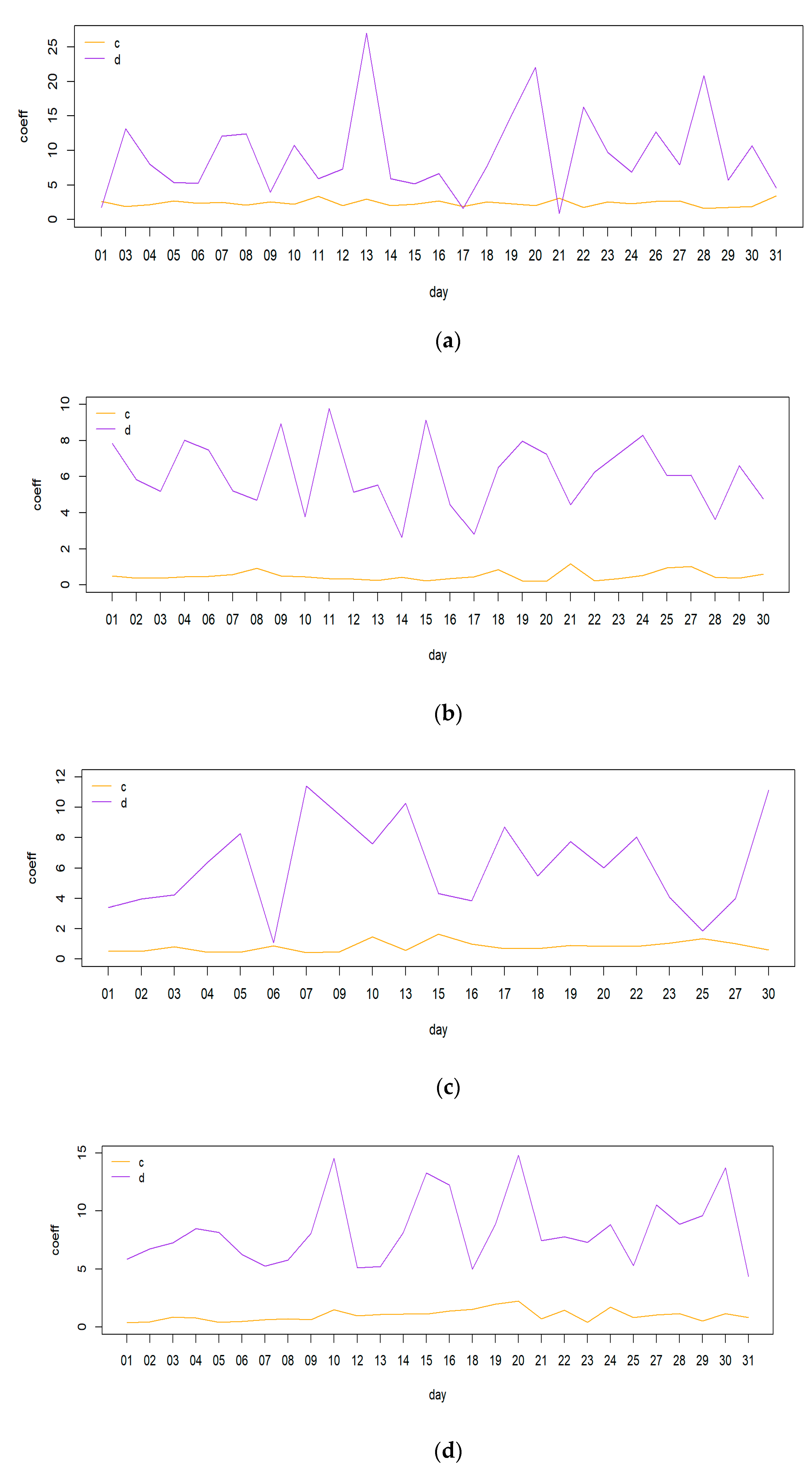
First, we compared the estimated variance coefficients to see if the EMOS model for LLWS is appropriate. Figure 8 gives time series of estimated variance coefficients, $\mathrm{c}\mathrm{and}\mathrm{d}$, for the same season (2019 MAM) and projection time at each airport. In Figure 8, the yellow line and purple line are the estimate c and d for projection time, respectively. As shown in the figure, it can be seen that the d values are relatively large compared to c values, implying that the non-homogeneous regression model or EMOS model is more suitable than the homogeneous regression model. For different seasons and projection times, the results were similar to those mentioned above.

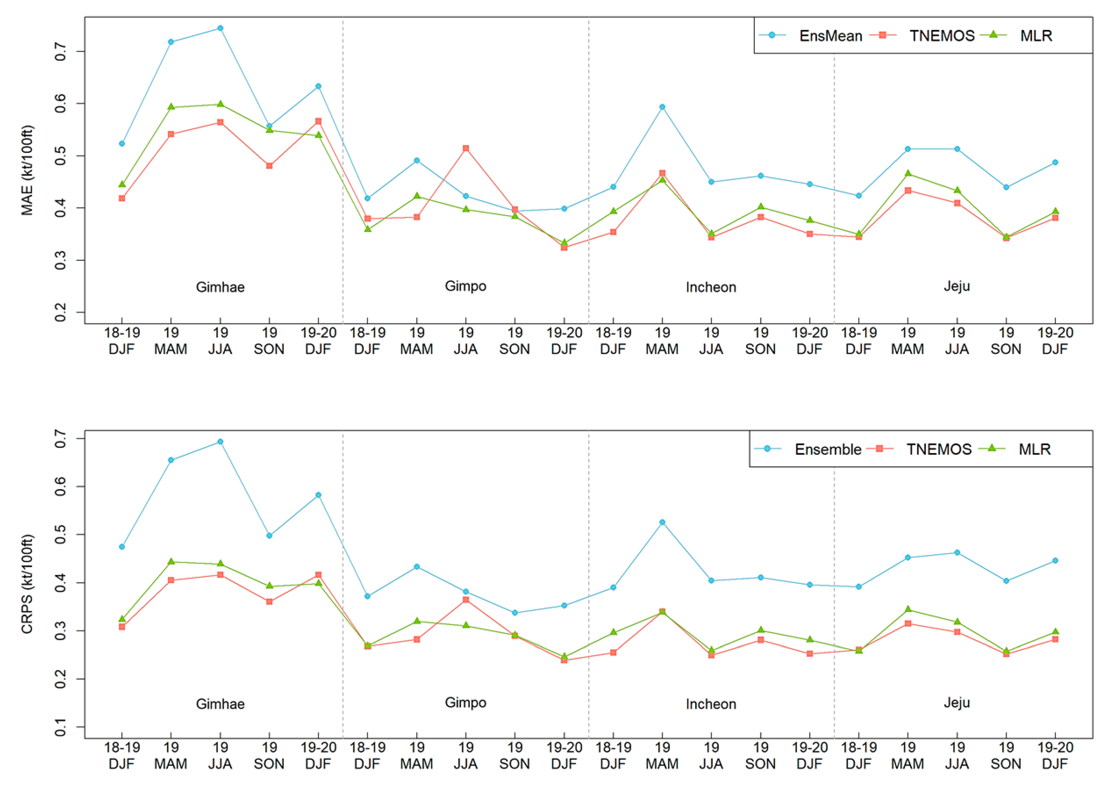
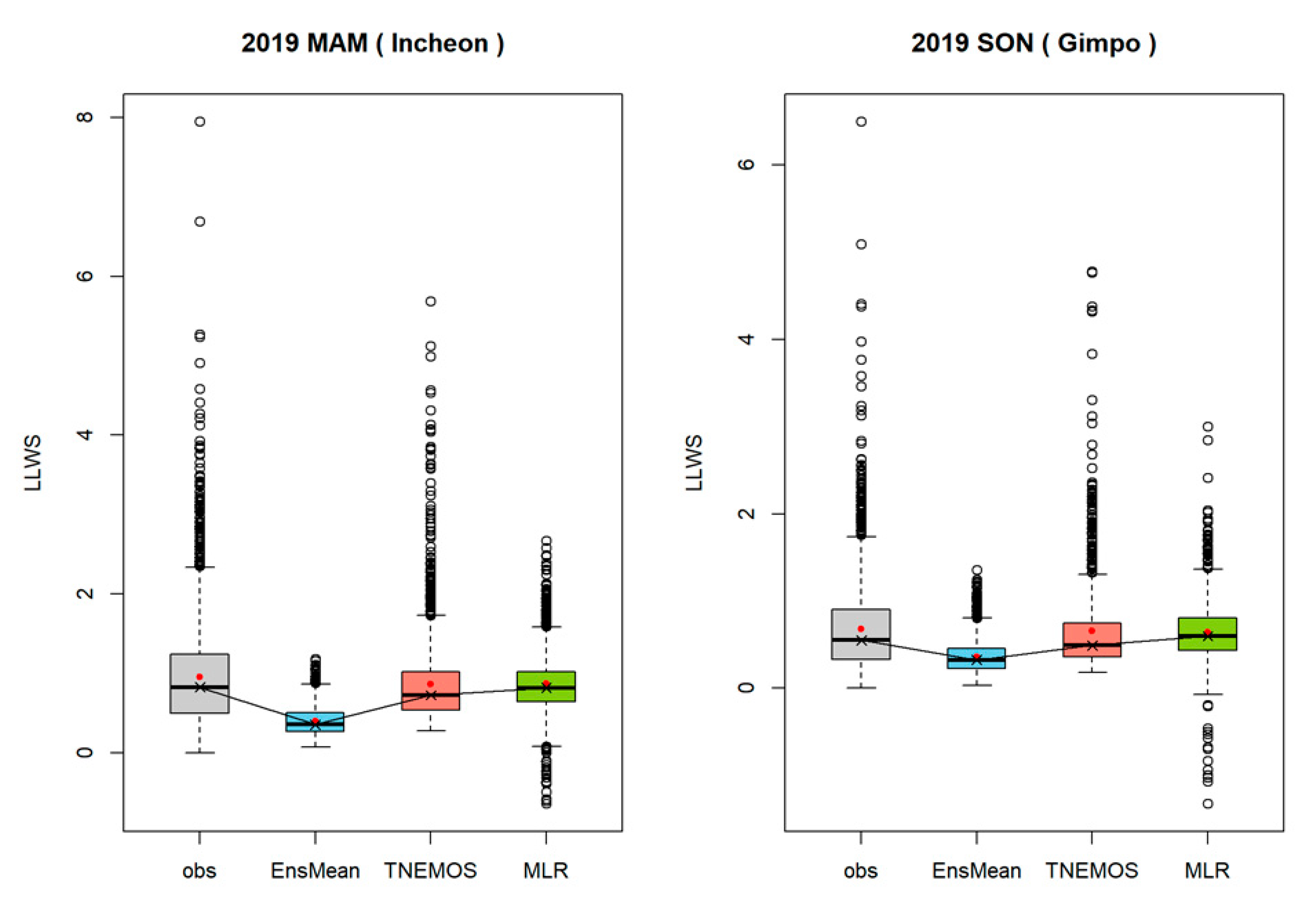
The prediction skills of the ensemble mean, multiple linear regression (MLR) and EMOS with a truncated normal distribution (TNEMOS) were compared in terms of MAE and CRPS, according to each season. The prediction errors of the ensemble mean, MLR and TNEMOS forecasts based on test datasets are given in Figure 9. It is seen that the prediction errors of MLR and TNEMOS forecasts have improved compared to the ensemble mean, although they are slightly different depending on the seasons and the airports. In addition, TNEMOS forecasts show better overall prediction performance than MLR in terms of MAE and CRPS. MLR forecasts can be estimated negative values due to the nature of the multiple regression model. These characteristics are illustrated by a box plot of the MLR given in Figure 10. In Figure 10, it can be seen that some of the estimates obtained by using MLR have values less than zero. When estimating probabilistic forecasts for weather variables with positive values, such as LLWS, it is not desirable to apply the multiple linear regression (MLR) model as it is. This is because the theoretical properties allow for the estimation of the real (or negative) values. Therefore, it shows that it is important to apply a model that reflects the characteristics of the data when applying a probabilistic forecast model.

For 2019 MAM of IIA and 2019 SON of GIA in Figure 10, it can be seen that TNEMOS forecasts are generally expected to be similar on average, but the variability is slightly smaller than the observations. In particular, since a number of outliers are occurring in the observations, predicting these outliers is one of the most important issues. If it is not possible to predict the case of high wind, the damage is bound to increase. Therefore, it can be seen that there is a limit to estimating these outliers, because the ensembles are too underestimated to predict such extreme values. However, it can be seen that outliers are estimated by the TNEMOS model and can provide very useful information compared to ensemble mean for predicting extreme values. It can also be seen that correcting for variability is more difficult than correcting bias. As shown in the figure, we can see that the ensembles are estimated to be relatively small compared to the observations and differ from the distributional characteristics of observations in general. On the other hand, TNEMOS forecasts tend to follow the distributional pattern of observations to some extent, albeit somewhat difference from observations, showing overall improved prediction performance over ensembles. Other airports and seasons showed similar patterns.

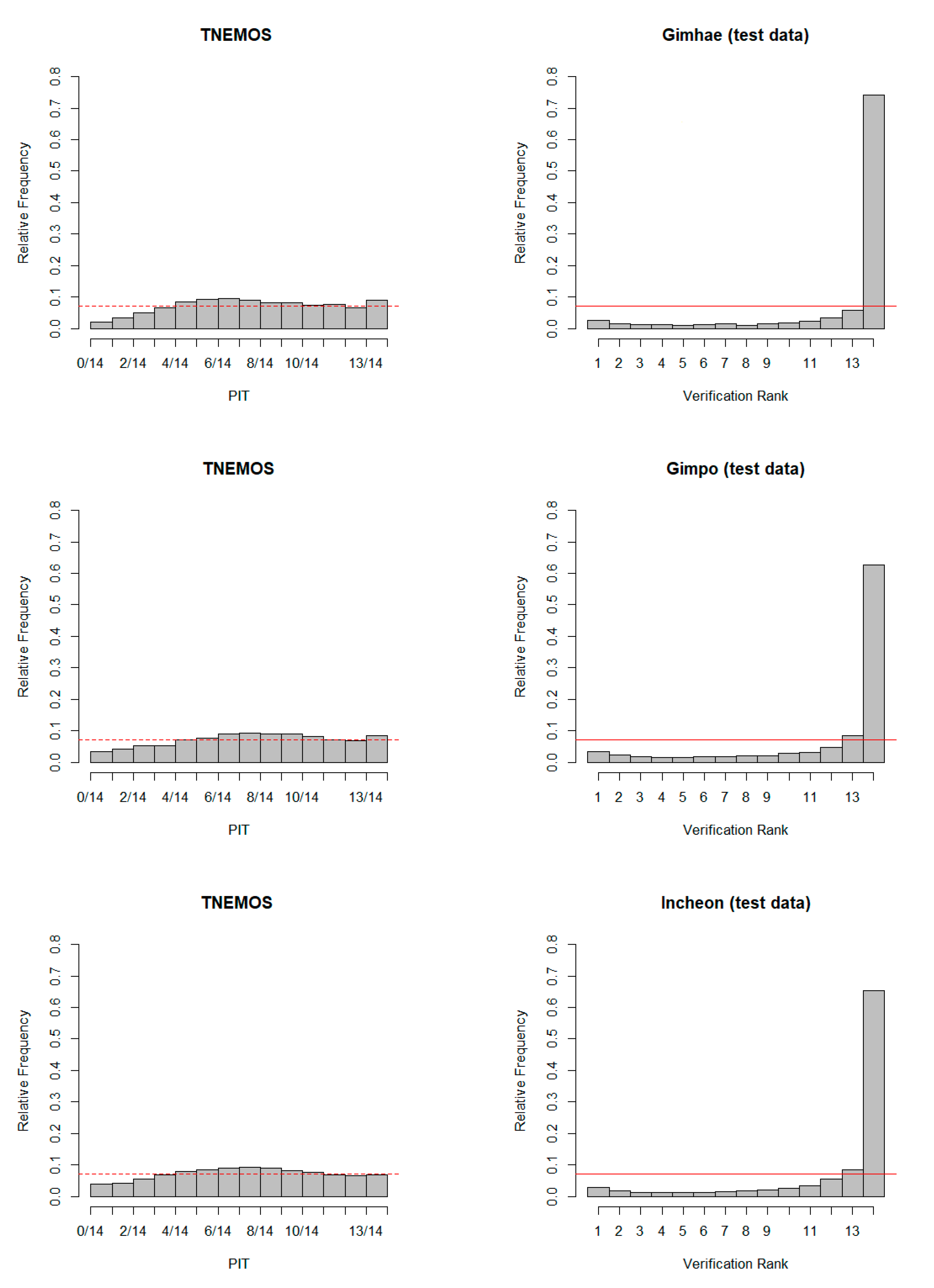
One of the visual tools for examining how well probabilistic forecasts are estimated is PIT (Probability Integral Transformation). PIT is a continuous random variable transformed by its own cumulative distribution function, which always has a standard uniform distribution. That is, the probabilistic forecasts estimated from the predictive probability density function have a good degree of prediction when the values transformed through the prediction cumulative probability distribution have a standard uniform distribution.

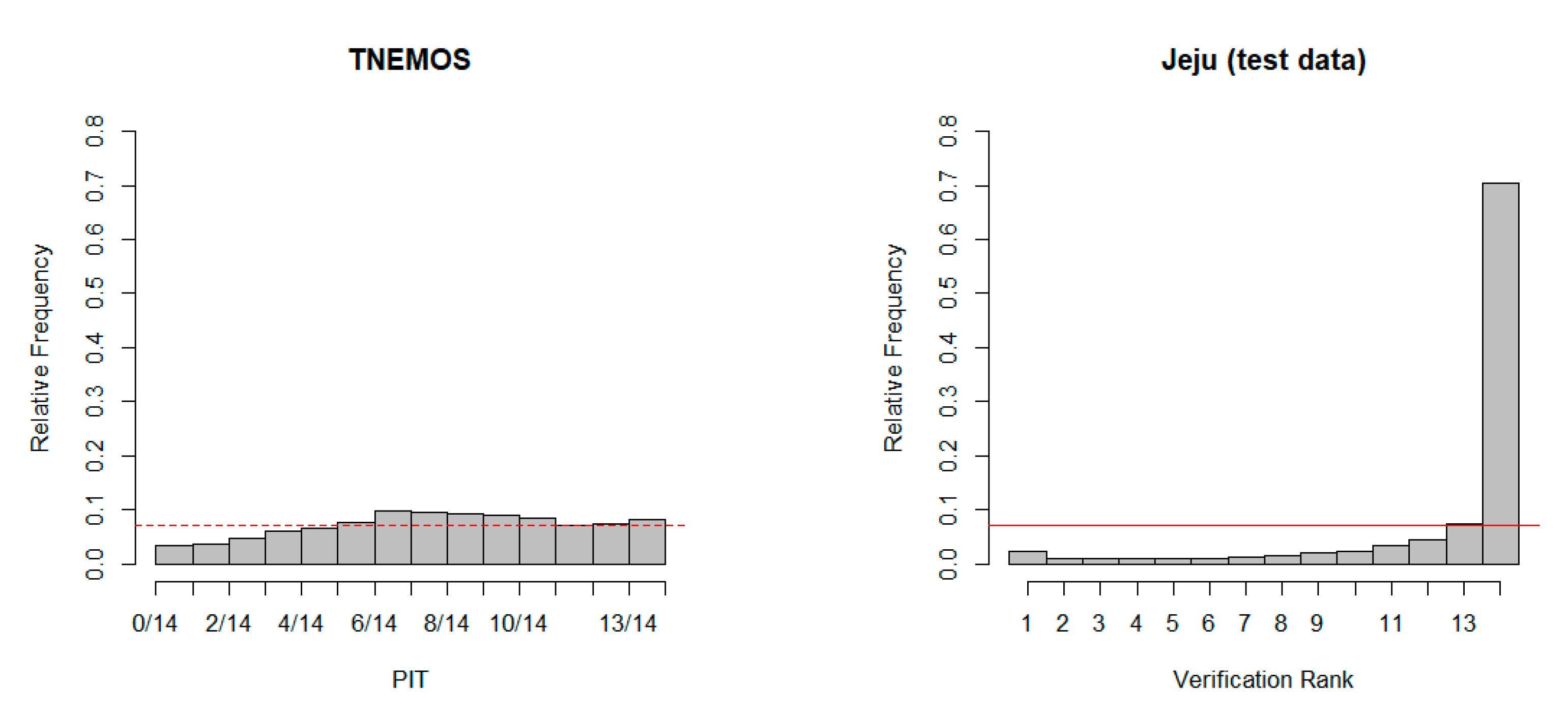
At each airport, a rank histogram for all data before applying a probabilistic forecast technique for a given verification period and a PIT histogram for all forecasts after applying TNEMOS are given to Figure 11. First, in the case of the rank histogram of Gimhae International Airport, it has a strong negative bias and shows a weak under-dispersion. The probabilistic forecast technique allows us to examine how much this trend and variability have improved through the PIT histogram. The PIT histogram of the estimated forecasts from the TNEMOS model shows that, although it does not have a completely uniform pattern, the trend and variability are generally calibrated rather than the rank histogram of the test period. In Gimpo, Incheon and Jeju International Airports, although somewhat different depending on airports, PIT histograms show generally even patterns, showing improved prediction performance over ensembles, and the probabilistic forecast technique provides useful ways to improve the accuracy and reliability of aviation variables.

Probabilistic forecast has an advantage of providing information about uncertainty, as it provides a way to quantify and predict the risk associated with weather prediction. That is, probabilistic forecasts are provided in the form of a predictive probability density functions for future weather quantities or events, so that the degree of occurrence of events of interest can be provided through the information of probability.

From the probabilistic forecast model for LLWS, we can estimate the predictive probability density function through Equation (3) for a given training period. From the estimated predictive probability density function, the probability of occurrence of a specific event of interest and 80% credible intervals are used to investigate a degree of prediction.

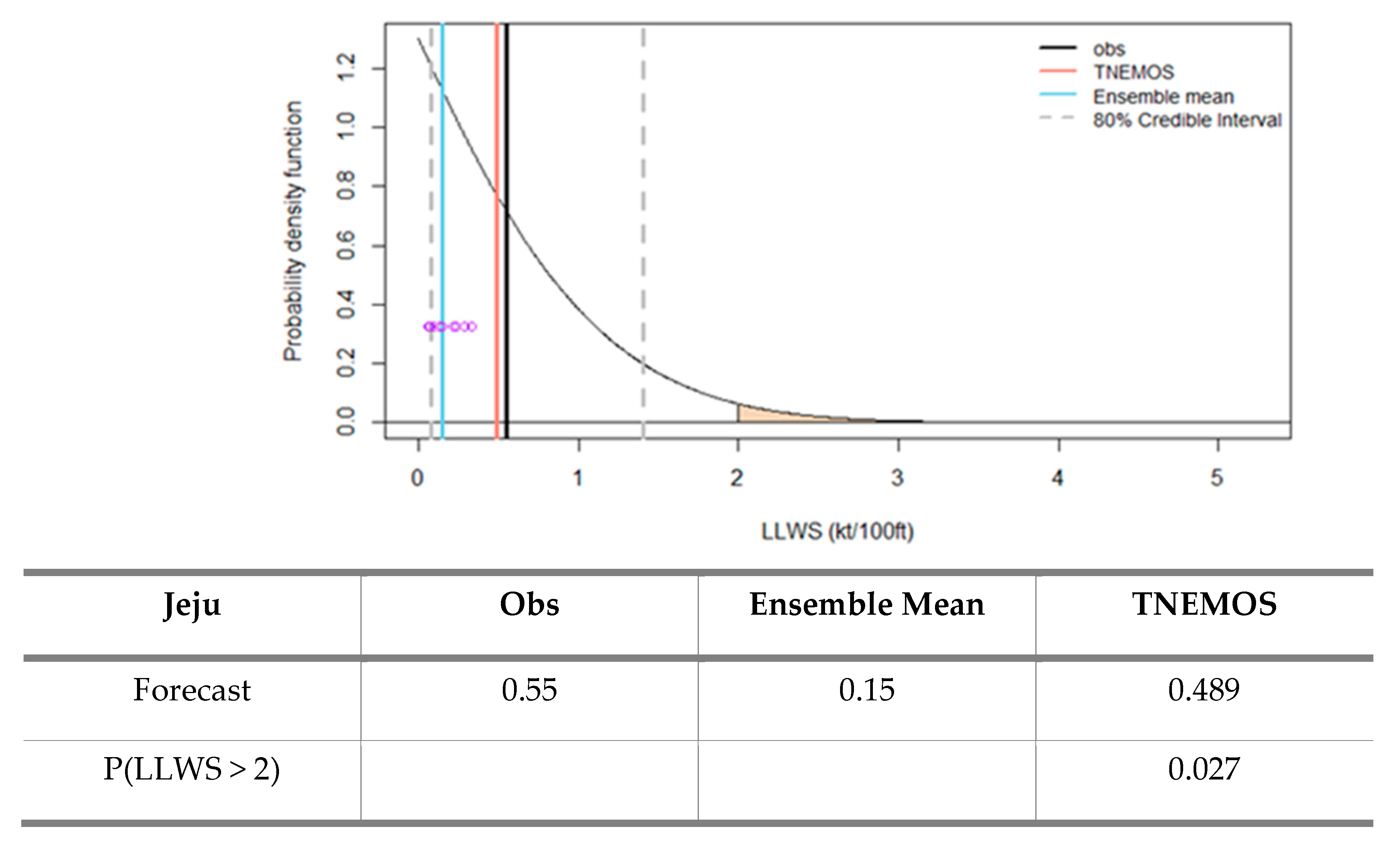
In Figure 12, the predictive PDF and 80% credible intervals for the projection time 5 h on 17 February 2020, at Jeju International Airport are given. The thin curve is the predictive PDF of LLWS, and the dots represent the ensemble member forecasts. The black vertical line is the verifying observation, the blue vertical line is the ensemble mean, the red vertical line is the TNEMOS forecast and the gray dotted lines are 80% credible intervals. The purple dots represent the ensemble member forecasts. As shown in the figure, the ensemble mean is included in the lower bound of 80% credible intervals, but it can be seen that the ensemble mean is predicted to be smaller than the observation. However, we can see that the TNEMOS forecast is predicted to similar to the observation. The yellow area of the predictive PDF shows how likely it is that a specific intensity of the LLWS will occur. In the figure, the probability of LLWS being more than 2 knots is 2.7%, indicating that this is unlikely to happen.

The predictive PDF and 80% credible intervals for the projection time 3 h on 22 February 2020 at Gimhae International Airport are given in Figure 13. In the figure, it can be seen that the ensemble member forecasts (purple dots) were simulated very small from LENS, and due to this effect, the ensemble mean was estimated to be 0.725. On the other hand, the observed LLWS was 3.86, showing a considerable difference. In this case, ensemble member forecasts were underestimated, and there is a limit to predicting LLWS by using the ensemble mean. Both the observation and probabilistic forecast of LLWS are contained in the 80% credible intervals, but the ensemble mean is located outside the lower bound of the credible intervals, which means that the degree of prediction is poor. The probability that the predicted LLWS is more than a certain threshold of 2 knots is 75.3%, which is highly likely to occur.

Since the probability information that occurs above a certain threshold from the predictive PDF is provided together with the forecast, it can explain to what extent or scale the prediction occurs, thus providing more available information to forecasters and users who utilize it.

As noted above, probability information obtained from the predictive PDF can account for uncertainty by providing additional information about the probability of occurrence compared to deterministic forecasts, thus providing useful information for aircraft operation and management.

5. Conclusions

The prediction of LLWS of Gimpo, Gimhae, Incheon and Jeju International Airports, using ensemble member forecasts generated from LENS, showed that the degree of performance was undesirable, due to the bias and dispersion inherent in the system. Therefore, statistical postprocessing techniques are needed to calibrate them.

In this study, we applied the EMOS model, which is one of the statistical postprocessing methods, and it provides a fully predictive density probability function for LLWS to reduce bias and dispersion. Since the non-negative values and an asymmetric distribution are allowed for LLWS, we used a left-truncated normal distribution with a cutoff at zero for LLWS as the predictive probability density function. In addition, since the properties or patterns of wind change according to the seasons, the probabilistic forecasts according to the seasons were estimated.

The results of the comparisons between the raw ensembles and probabilistic forecasts revealed that probabilistic forecasts exhibited better prediction skills in terms of MAE, CRPS and PIT for all seasons. Therefore, the system error and dispersion owing to the limitations and the uncertainty of its model can be reduced significantly by applying the EMOS model. Moreover, probability information obtained from the predictive PDF can account for uncertainty by providing additional information about the probability of occurrence compared to deterministic forecasts, thus providing useful information for aircraft operation and management.

The bias and uncertainty were quantified by estimating probabilistic forecasts to provide more reliable and accurate information of LLWS according to the seasons. However, it can be seen that the prediction skills have room for improvement, due to the training period, seasons, ensemble models, etc. Although this study focused only on EMOS with a left-truncated normal distribution, further improvements in ensemble calibration can be provided by comparative study of models reflecting various other distributions or other techniques.