Numerical Investigation of Track and Intensity Evolution of Typhoon Doksuri (2023)

Abstract

This study utilized the WRF model to investigate the track evolution and rapid intensification (RI) of Typhoon Doksuri (2023) as it moved across the Luzon Strait and through the South China Sea (SCS). The simulation results indicate that Doksuri has a smaller track sensitivity to the use of different physics schemes, while having a greater intensity sensitivity. Sensitivity numerical experiments with different physics schemes can well capture its northwestward movement in the first two days, but they predict less westward track deflection as the typhoon moves across the Luzon Strait and through the SCS. Moreover, all the experiments successfully simulated Doksuri’s RI, albeit with quite different rates and a time lag of 12 h. Among different combinations of physics schemes, there exists an optimal set of cumulus parameterization and cloud microphysics schemes for track and intensity predictions. Doksuri’s track changes as the typhoon moved across the Luzon Strait and through the SCS were influenced by the topographic effects of the terrain of the Philippines and Taiwan, to different extents. The track changes of Doksuri are explained by the wavenumber-one potential vorticity (PV) tendency budget from different physical processes, highlighting that the horizontal PV advection dominates the PV tendency throughout most of the simulation time due to the offset of vertical PV advection and differential diabatic heating. In addition, this study applies the extended Sawyer–Eliassen (SE) equation to compare the transverse circulations of the typhoon induced by various forcing sources. The SE solution indicates that radial inflow was largely driven in the lower-tropospheric vortex by strong diabatic heating, while being significantly enhanced in the lower boundary layer due to turbulent friction. All other physical forcing terms were relatively insignificant for the induced transverse circulation. The coordinated radial inflow at low levels may have led to the eyewall development in unbalanced dynamics. Intense diabatic heating thus was vital to the severe RI of Doksuri under a weak vertical wind shear.

1. Introduction

Tropical cyclones (TCs) are low-pressure systems that form over warm tropical oceans. They are natural disasters that inflict substantial property damage and human casualties over expansive regions in a relatively brief period due to strong winds and heavy rainfall. Thus, accurate track and intensity forecasting, thorough preparedness, and timely responses are essential for reducing property damage and preventing casualties caused by TCs. The reliability of numerical weather prediction (NWP) models plays a pivotal role in forecasting and guiding decision-making during TC events. With ongoing advancements in modeling techniques, the accuracy of TC predictions has markedly improved in recent decades. Emanuel et al. [1] highlighted notable progress in TC track forecasting over the past thirty years. Cangialosi et al. [2] reported that the forecast error for 72 h decreased from an average of about 240 km (from 1990 to 1999) to 150 km (from 2000 to 2009), and then to 100 km (from 2010 to 2019). They also indicated that for 120 h, the forecast error decreased from an average of about 265 km (from 2000 to 2009) to 185 km (from 2010 to 2019). Furthermore, there have been consistent enhancements in 24 h forecast accuracy for typhoon tracks, with errors reduced to approximately 50 km [3,4]. In addition to significant advancements in forecasting TC tracks, there have also been improvements in intensity forecasts. Recently, there has been a significant reduction in forecast errors for TC intensity and an improvement in intensity forecasting accuracy [2]. However, accurately predicting the intensity of TCs remains a formidable challenge [2,5,6], particularly for TCs undergoing rapid intensification (RI). RI is characterized by a central sea-level pressure drop greater than 42 hPa per day for TCs over the western North Pacific (WNP) [7], or a maximum 10 m wind speed increase of 30 kt in one day for TCs over the Atlantic [8].

The Weather Research and Forecasting (WRF) model has integrated numerous alternative physical parameterization schemes to capture various atmospheric processes, making it an important tool for numerical weather prediction. Additionally, the model allows for the flexible integration of schemes representing different physical processes, enabling a comprehensive representation of atmospheric dynamics. Li et al. [9] investigated the effects of different cumulus physics schemes on WRF’s representation of typhoon precipitation. Additionally, several other investigations have explored the impact of combining schemes for cloud microphysics and the planetary boundary layer on track forecasts of TCs [10,11]. Moreover, combinations of schemes from all three physics components, namely cumulus, microphysics, and the planetary boundary layer, have been explored [5,12].

The simulated track and intensity of TCs can change considerably when using different combinations of physics parameterization schemes in the model [13,14,15,16]. Cloud microphysics, cumulus parameterization, and the planetary boundary layer have a greater influence on simulated TC track and intensity compared to other parameterizations [12,13]. The cumulus parameterization scheme (CPS) addresses the subgrid-scale effects of convective and/or shallow clouds by incorporating vertical fluxes generated by unresolved updrafts and downdrafts, along with compensatory motions occurring outside of clouds. Conversely, the microphysics parameterization scheme (MPS) explicitly integrates resolved processes concerning water vapor, cloud formation, and precipitation. Enhancing the understanding of these physical parameters will result in improved predictions of TC track and intensity.

TC track prediction is influenced by the complex interaction between the large-scale environmental circulation and the vortex circulation itself. The primary concept in the theory and forecasting of TC motion is “steering” by the environmental flow. However, this movement is modified by the Coriolis force (the beta effect) and the horizontal vorticity gradient of the surrounding flow [17]. As a TC approaches terrain, its track becomes more complex [18,19,20,21,22]. Additionally, the relationship between TC motion and sea surface temperature (SST) has been studied, revealing that SST variations also impact TC track and intensity [23,24,25,26].

To deepen the understanding of the influence of physical processes on TC motion, Wu and Wang [27] introduced a new dynamical framework of potential vorticity (PV) tendency. They showed that TCs tend to move towards regions where the azimuthal wavenumber-one component reaches its peak. Additionally, Tang et al. [18] used the PV tendency budget and found that the differential diabatic heating term becomes comparable to horizontal PV advection. Li and Huang [20] pointed out that the southward deflection of Typhoon Megi during landfall resulted from the southeastward movement of the diabatic heating effect. Meanwhile, Hsu et al. [28] applied the PV tendency budget to examine the impacts of horizontal and vertical PV advection alongside diabatic heating, revealing that the leftward turn of typhoons near landfall is predominantly influenced by vertical PV advection and diabatic heating.

The Sawyer–Eliassen (SE) equation, a linear partial differential equation, is widely used to analyze the transverse circulation and intensification processes of simulated TCs under different forcing sources [29,30,31,32,33]. Generally, the SE equation exists in two primary forms: the original SE equation [29,31], which rests upon thermal wind balance, and the extended SE equation [32,33], which relaxes the thermal wind balance. Ji and Qiao [32] demonstrated that the unbalanced solution of the extended SE equation captures the transverse circulation and boundary layer inflow more accurately than the balanced solution [29,31,34] and pseudo-balanced solution [30] for the original SE equation. In addition, Nguyen and Huang [33] utilized the extended SE equation, as introduced by Ji and Qiao [32], to investigate the effects of residual terms on the induced transverse circulation associated with a real super-intense typhoon. They found that incorporating these residual terms resulted in an induced transverse circulation that closely resembled the nonlinear simulation.

Typhoon Doksuri first appeared as a low-pressure area in the Philippine Sea, far off the eastern coast of Mindanao, on 19 July 2023. The system intensified into a tropical storm on 21 July and slightly intensified as it moved northwestward on the following day. At 0900 UTC on 23 July, Doksuri began to rapidly intensify, reaching typhoon status over the Philippine Sea. According to the International Best Track Archive for Climate Stewardship (IBTrACS), its maximum sustained wind speeds increased by approximately 20 m s⁻¹ over 24 h, from 1200 UTC on 23 July to 0600 UTC on 24 July, eventually peaking at 65 m s⁻¹ at 0600 UTC on 24 July. As Doksuri approached the northernmost part of the Philippines, it significantly slowed down. By around 1200 UTC on 25 July, the storm was located just off the coast northwest of Cagayan, moving westward through the Luzon Strait. Doksuri left the Philippine Area of Responsibility at around 0200 UTC on 27 July, resuming its northwestward to north-northwestward movement. It ultimately made landfall in Fujian, China, on 28 July.

Doksuri took a northwestward to more northward movement northeast and north of the Philippines to the southwest of Taiwan, illustrating a curved track with an intermediate RI worthy of dynamic investigation. The asymmetric structure of the PV tendency budget is used to examine the dynamic processes involved in the track changes of Doksuri. Additionally, we have solved the extended SE equation to explore the contributions of different forcing sources to the induced transverse circulation of the primary mean vortex for Typhoon Doksuri during the RI period. Section 2 introduces the WRF model and sensitivity experiments for Doksuri. In Section 3, simulation results of sensitivity experiments with different cumulus parameterizations and cloud microphysics schemes are explored, identifying the optimal combination of schemes for further analysis. Section 4 analyzes the vortex dynamics to understand the mechanisms associated with track changes. In Section 5, we focus on the mechanisms for vortex intensification during the RI period. Finally, conclusions are presented in Section 6.

2. Model Configuration and Numerical Experiments

2.1. Model Settings

The Weather Research and Forecasting (WRF) model version 4.2.1 [35] was used to simulate Typhoon Doksuri. WRF is currently utilized operationally at the National Centers for Environmental Prediction (NCEP) and other national meteorological centers, as well as in real-time forecasting setups at laboratories, universities, and companies. In this study, the model simulations utilized two nested domains with horizontal resolutions of 15 km (617 × 514 grid points) and 3 km (956 × 881 grid points), respectively (Figure 1). A two-way nesting approach was adopted, allowing the finer domain’s solution to update the coarser domain’s solution within their overlapping region. Both domains included 52 vertical levels, with the model top set at 20 hPa. The initial and boundary conditions for the WRF simulation were obtained from the NCEP Global Data Assimilation System (GDAS) Final Analysis, which has a horizontal resolution of 0.25° × 0.25° and a temporal resolution of 6 h. Doksuri traveled over a region of warm SSTs around 29–30 °C along its track. The SST remained unchanged in all the simulations.

2.2. Sensitivity Experiments

The simulation period for Doksuri was from 1200 UTC 23 July to 1200 UTC 28 July 2023 for a total of 120 h. To investigate the sensitivity of typhoon simulations to CPS, four different CPSs, including the Kain–Fritsch (KF), Grell–Freitas Ensemble (GF), Grell 3D Ensemble (GD), and New Tiedtke schemes, were compared. Meanwhile, fifteen MPSs, including Lin, WRF single-moment three-class (WSM3), WRF single-moment five-class (WSM5), WRF single-moment six-class (WSM6), Goddard, Thompson, Milbrandt–Yau double-moment (Milbrandt-Yau), Morrison two-moment (Morrison 2), Stony Brook University (Stony-Brook), WRF double-moment five-class (WDM5), WRF double-moment six-class (WDM6), National Severe Storms Laboratory two-moment (NSSL2), National Severe Storms Laboratory one-moment (NSSL1), and Predicted Particle Properties (P3) schemes, were used to investigate the sensitivity of the model simulations to MPS. More details about the options of the physics schemes for numerical simulations are listed in

Table 1. The options of physics schemes for numerical simulations.

Physics Options	Schemes
Microphysics parameterization scheme (MPS)	Lin [38]
	WSM3 [39]
	WSM5 [39]
	WSM6 [40]
	Goddard [41]
	Thompson [42]
	Eta [43]
	Milbrandt-Yau [44]
	Morrison 2 [45]
	Stony-Brook [46]
	WDM5 [47]
	WDM6 [47]
	NSSL2 [48]
	NSSL1 [49]
	P3 [50]
Cumulus parameterization scheme (CPS)	KF [51]
	GF [52]
	GD [53]
	New Tiedtke [54]
Planetary boundary layer (PBL) physics scheme	Yonsei University [55]
Shortwave scheme	Dudhia [56]
Longwave scheme	RRTM [57]

. Note that the CPSs and MPSs used in this study are the popular physics schemes in the WRF model and have been extensively applied in numerous prior studies for TC simulations [15,36,37]. The first was a combination of six different MPSs (Lin, WSM6, Goddard, Thompson, NSSL2, and P3) with four different CPSs to select the best CPS for the track and intensity simulations. Later on, we used the best CPS combined with the other nine MPSs to choose the best MPS for track and intensity. Our treatment without a complete sampling was mainly to reduce the computational cost. Thus, the best choice among the experiments for CPS and MPS was determined to be the “optimal” scheme combination for the simulation of Typhoon Doksuri. Herein, it was not intended for a predictability problem, but rather suited to an investigation of dynamic mechanisms with reasonably simulated track and intensity.

3. Simulation Results of Sensitivity Experiments

3.1. Simulation Sensitivity to Cumulus Parameterization Schemes

To investigate the impacts of different physics schemes on the prediction of typhoon track and intensity for Typhoon Doksuri, we conducted several experiments with different cloud microphysics schemes (including Lin, WSM6, Goddard, Thompson, NSSL2, and P3) and CPSs (including KF, GF, GD, and New Tiedtke). The details of the physics schemes are listed in Table 1. Figure 2 shows the simulated tracks and intensities for these sensitivity experiments using a combination of the four different CPSs and the six different MPSs above; the best tracks from IBTrACS and JMA for Typhoon Doksuri are also included for comparison. During the simulation period from 1200 UTC 23 July to 1200 UTC 28 July 2023, Typhoon Doksuri initially moves northwestward across the Philippine Sea, then proceeds westward through the Luzon Strait, and eventually shifts northwestward to north-northwestward across the South China Sea (SCS) near Taiwan. It was evident that the physics schemes had a relatively small influence on the track simulations for Doksuri. All the experiments reasonably simulated the track of Doksuri in the first two days; however, they exhibited northward deviations thereafter. Notably, the GF cumulus scheme (Figure 2b) depicted Doksuri’s track slightly better than the other CPSs (Figure 2a,c,d), showing reduced northward deviation in the last three days of the forecast. Among the tests, the experiment using the GF cumulus scheme with the NSSL2 microphysics scheme (highlighted in red in Figure 2) showed a relatively better track forecast on the third day with the smallest northward deviation. In conclusion, the GF cumulus scheme, particularly when combined with the NSSL2 microphysics scheme, produced track forecasts that agree better with the best track data for Typhoon Doksuri.

In contrast to the track simulations, the intensity simulations for Doksuri exhibited greater sensitivity to different physics schemes (Figure 2e–h). The time evolution of the typhoon intensity showed that all the experiments successfully captured the RI in the first 36 h but with a time lag of 12 h, and they failed to capture the re-intensification process from 84 to 96 h over the SCS. Note that the RI ceases as the typhoon nears the north of the Philippines to deflect further northward. For the cloud microphysics schemes, the value of the 10 m maximum wind speed (V_max) for the Lin, WSM6, and Thompson schemes was significantly smaller than the best track value from IBTrACS during the RI period. Conversely, the value of V_max for the Goddard, NSSL2, and P3 schemes closely matched the best track value from IBTrACS, except for when combined with the GD cumulus scheme (Figure 2g). Indeed, the KF, GF, and New Tiedtke cumulus schemes gave a better performance of V_max than the GD scheme, closer to IBTrACS data during the first 36 h. Therefore, Typhoon Doksuri shows relatively less track sensitivity to the use of different physics schemes but a greater sensitivity for the intensity prediction, similar to supertyphoon Mangkhut (2018) [58]. The cloud microphysics scheme NSSL2, in general, gave the strongest intensity with a reasonable prediction of V_max. Thus, the GF cumulus scheme stood out as the best-performing CPS for both track and intensity simulations. We also tested the deactivation of the CPS and found that the overestimation due to the cumulus effect in the inner domain was not prominent for this case. With the CPS activated, the model successfully captured the RI of Doksuri without over-prediction.

3.2. Simulation Sensitivity to Cloud Microphysics Schemes

To further investigate the performances of MCPs in simulations, Figure 3a,b present the simulated tracks and intensities from the sensitivity experiments using the combination of the GF cumulus scheme and the other nine MPSs (including WSM3, WSM5, Eta, Milbrandt, Morrion, StonyBrook, WDM5, WDM6, and NSSL1, see Table 1). The simulated tracks of Doksuri for all the sensitivity experiments compare well with the best track from IBTrACS, except for the last day of the forecast (Figure 3a). Indeed, the model reasonably captures the translating directions of Typhoon Doksuri, but with a slightly northward deviation. For typhoon intensity, most of the sensitivity experiments showed significantly smaller magnitudes of V_max than the best track data from IBTrACS during the RI period and also could not capture the re-intensification of typhoon over the SCS (Figure 3b).

Figure 3c shows the simulated track errors from the sensitivity experiments combining the GF cumulus scheme with all the fifteen different MPSs, as in Table 1. The simulated track errors were primarily caused by differences in the forecasted translation speeds of Doksuri, which moved faster than observed, particularly after 48 h. The findings highlight that the NSSL2 microphysics scheme produced the best result, with a smaller track error than other schemes, except for the Eta scheme. However, as evident in Figure 3b, the Eta scheme obtained a rather poor intensity forecast compared to the IBTrACS intensity. For the simulated results of track and intensity, the combination of the GF cumulus and NSSL2 microphysics scheme not only could capture the RI during the first two days but also provided better track simulation compared to others. Thus, the NSSL2 scheme was superior compared to the fourteen other schemes. This combination experiment was selected as the control run (CTL) for further analysis. Note that the sensitivities of both TC track and intensity forecasts to various cumulus and cloud microphysics schemes have been explored by many papers for various TCs. Our interest, however, was on the curved track and RI of Typhoon Doksuri when the typhoon moves across the Luzon Strait and through the SCS. Therefore, we concentrate on the CTL experiment in the following sections.

The NSSL2 microphysics scheme given by Mansell et al. [48] uses a double-moment approach similar to WDM6. This is a bulk scheme that predicts the mass mixing ratio and number concentrations of cloud droplets, rain, ice crystals, snow, and graupel. It provides a more accurate representation of the size distribution and number concentration.

3.3. Simulated Precipitation

CTL well captured the translation direction of Doksuri in the first two days, as seen in Figure 2f. It is of great interest to show the simulated rainfall of the typhoon to reveal the activity of cloud convection. Figure 4 shows the simulated hourly accumulated rainfall of CTL from 12 to 48 h at intervals of 12 h. The rainfall observation available for verification is the hourly rainfall from the multi-satellite precipitation product from Jaxa (GSMaP) during the same simulation times. In general, the rainfall areas of GSMaP and CTL were similar and consistent with satellite images (figures not shown). However, the simulated precipitation from CTL was higher than that observed by GSMaP, particularly around the inner typhoon. The simulated heavy rainfall from CTL at 36 and 48 h over the northern Philippines was similar to GSMaP when the typhoon flow was impacted by the orographic lifting of the Philippines terrain, thus with increasing convection in this area (Figure 4c,d,g,h). The simulated accumulated rainfall also highlighted the primary region of latent heating associated with the typhoon across the Luzon Strait and through the SCS. Although the simulated convection associated with the intense typhoon was considerably stronger than the satellite observations (normally underestimated), their overall features (e.g., the eye, eyewall, and spiral clouds) were similar, except for some weakened convection over the north Philippines at 48 h.

4. Analysis for Track Deflection

4.1. Circulation Structure

The evolution of the simulated horizontal wind and vertical velocity illustrates the typhoon’s translation and convection. Figure 5 shows that the simulated typhoon circulations averaged from 1 to 8 km at 36, 48, 60, and 72 h for CTL. As the simulated typhoon track shifts from west-northwestward to westward movement between 36 and 48 h, a stronger easterly wind develops north-northeast of the typhoon center (Figure 5a,b), accompanied by relatively more symmetrical vertical motions (Figure 5e,f). When Doksuri moves across the Luzon Strait, the vertical motions are influenced by the terrain. At 60 h, the east-southeasterly wind north-northeast of the typhoon center weakens compared to 48 h (Figure 5c). At this stage, while the horizontal wind is relatively more symmetric, the vertical motions exhibit a more asymmetric structure (Figure 5g), with stronger upward motions primarily in the west and east quadrants of the inner vortex. As the typhoon moves across the SCS, high-wind-speed zones again occur in the northeast of the inner vortex to induce a more northwestward component (Figure 5d). However, the upward motions now remain concentrated strongly in the west and east quadrants of the inner vortex (Figure 5h). The induced flow asymmetry, driven by the enhanced southeasterly wind, tends to steer the typhoon more northwestward.

To illustrate the relation between the typhoon circulation and track evolution for Doksuri, Figure 6 shows the time evolutions of the simulated horizontal velocity, vertical velocity, and diabatic heating in the inner core concerning azimuthal variations from 0 to 96 h. Before 48 h, when the typhoon has a northwestward movement, stronger wind speeds are observed primarily northeast of the typhoon center (Figure 6a), accompanied by relatively symmetrical upward motions and diabatic heating (Figure 6b,c). When the typhoon moves across the Luzon Strait, the stronger horizontal wind speed rotates counterclockwise to the north of the typhoon center, and the wind speed weakens (Figure 6a), which tends to steer the typhoon more westward. During this period, the upward motions and diabatic heating remain a relatively more symmetric structure (Figure 6b,c). As the typhoon moves across the SCS (from 60 to 84 h), the horizontal velocity becomes stronger east of the typhoon center in response to its northwestward movement in concordance with Figure 5c,d. At this time, the stronger upward motions and diabatic heating are in phase and rotate counterclockwise from the northwest (at 60 h) to the south (at 84 h) of the typhoon center. Therefore, significant differences exist in the flow asymmetry and convection of Doksuri as it moves across the Philippine Sea, Luzon Strait, and the SCS.

4.2. Dynamics of Track Evolution

The asymmetric structure of the PV tendency budget can be used to examine the dynamic processes involved in the track changes of a typhoon [20,58]. The equation for the PV budgets is following [58]. To further understand the contributions of different physical processes to the vortex translation throughout the entire forecast time, Figure 7 shows the time evolutions of their induced translations, inferred from the net wavenumber-one (WN-1) PV tendency budget, for Doksuri during its simulation period. These induced translations agree well with the actual movement of CTL shown earlier. Throughout most of the simulation time before 72 h, the horizontal PV advection roughly dominates the PV tendency when the contributions from vertical PV advection and differential diabatic heating are not significant. Indeed, the northwestward translation of Doksuri before 48 h and the subsequent westward translation after 48 h are largely driven by the strongest horizontal PV advection. After 72 h, vertical PV advection and differential diabatic heating somewhat contribute to the typhoon’s movement, but both effects nearly cancel out. Consequently, the northwestward translation of Doksuri as it moves farther from Luzon Island remains primarily determined by the strongest horizontal PV advection, consistent with previous studies [58]. Note that both environmental flow and inner vortex core provide a steering of the vortex. For WN-1 components, the environmental flow is the basic flow embedding the vortex. Herein, the asymmetry of the inner core includes both flow components, thereby reflecting the fact that horizontal PV advection is more important for the vortex translation. In summary, the translation of CTL is essentially driven by horizontal PV advection at most of the time. This is due to the insignificant contributions of vertical PV advection and differential diabatic heating before 72 h, and their offsetting effects after 72 h.

4.3. Track Forecast without Terrain

As Typhoon Doksuri approached the terrain of the Philippines and Taiwan, its track underwent significant changes. Initially, it moved northwestward across the Philippine Sea, then shifted westward through the Luzon Strait, and eventually took a northwestward to north-northwestward path across the SCS near Taiwan. Thus, it was of great interest for us to underline the relative impacts of both terrains on the track evolution of Doksuri at different stages in this study by conducting terrain sensitivity experiments. In the NoTW (without Taiwan terrain), NoPhi (without Philippines terrain), and NoPhi-TW (without Philippines and Taiwan terrain) experiments, the terrain of the entire Philippines or Taiwan, or both, was reset to a plain. Figure 8 shows the simulated tracks for CTL, NoPhi, NoTW, NoPhi-TW, and the best track data from IBTrACS. The track changes of all the sensitivity experiments after 48 h indicated that the track of Doksuri was somewhat sensitive to the Philippines and Taiwan terrains. Indeed, compared to CTL, NoTW slightly increased the northward deviation offshore of the northern Philippines before 72 h. In addition, NoPhi also resulted in a more northward deviation than CTL, leading Doksuri to make landfall in Taiwan before reaching South China. When both the Philippines and Taiwan were set to plain, the typhoon consistently maintained a northwestward translation most of the time. This suggests that the changes in Doksuri’s direction as it traversed the Luzon Strait and moved through the SCS near Taiwan were also influenced by the terrain at these oceanic regions.

Similar to Figure 7, Figure 9 shows the contributions of different physical processes to the vortex translation of NoPhi and NoTW throughout the entire forecast times. Similar to CTL, the induced translations of NoTW and NoPhi agreed with their actual movements. For NoTW, the contribution of differential diabatic heating to the typhoon’s movement was more significant than in CTL (Figure 9a). NoTW failed to capture the westward translation during 48–60 h period (see Figure 7) that was mainly due to a northward to northeastward movement induced by the differential diabatic heating. Additionally, NoTW did not capture the north-northwestward movement on the last day, which was primarily due to northwestward movement contributed by horizontal PV advection. Resetting the Philippines terrain to a plain had only small impacts on vertical PV advection. For NoPhi, the contributions from vertical PV advection and differential diabatic heating were almost insignificant to the typhoon’s movement during most of the forecast times (Figure 9b). Therefore, the northward deflection of the typhoon after 48 h was mainly due to the contribution from horizontal PV advection. Notably, differential diabatic heating became more important for the northwestward movement of the typhoon during 24 to 48 h, contributing to a northward track. When the terrain of the entire Philippines or Taiwan was reset to a plain, it affected TC by altering their interactions with surrounding atmospheric conditions. Different terrains influence a TC circulation through various factors, including surface characteristics, moisture availability, wind patterns, and atmospheric dynamics. These factors modify the heating and cooling processes, which subsequently impact the structure, track, and intensity of the TC. As a result, diabatic heating, horizontal PV advection, and vertical PV advection are changed with different terrains. The terrain sensitivity experiments highlighted the typhoon track evolution in relation to PV dynamics that was not illustrated for similar typhoons by other published papers.

5. Dynamics on Typhoon Intensity

The simulated intensity evolution for CTL clearly shows that Doksuri underwent a fast intensification during the first two days. Specifically, the simulated intensity of Doksuri increased by 27 m s⁻¹ within the first 24 h (from 0 to 24 h) and experienced a further intensification of about 15 m s⁻¹ within 12 h (from 36 to 48 h) as a severe RI. In the next section, we will focus on our investigation of the RI process of Doksuri during the first two days of the CTL experiment.

5.1. Thermodynamic Conditions

Figure 10 shows the LHF at different times from 3 to 48 h for CTL, overlapped with their VWS. At 3 h, the higher LHF is only concentrated in a small region in the northwest quadrant of the typhoon center with a maximum value of about 900 W m⁻² (Figure 10a). As RI is in progress, the LHF becomes more circularly shaped and stronger. (Figure 10b–f). Indeed, the LHF can reach a maximum value of over 1200 W m⁻² at 48 h when the typhoon intensity becomes strongest, covering nearly all the areas surrounding the typhoon center (Figure 10f). Throughout the RI process, the LHF is predominantly concentrated within a radius of 100 km from the typhoon center. The large release of LHF from 24 to 48 h coincides with an increase in vertical vorticity, indicating that strong upward motions with the abundant release of LHF can further strengthen the transverse circulation. Additionally, vertical wind shear (VWS), represented by vectors in each figure, remains relatively small during this period, mostly below 4.7 m s⁻¹. This low VWS is a favorable condition for the intensification of Doksuri.

The transverse circulation can be largely driven by the effect of diabatic heating in the developing typhoon. Figure 11 shows the evolution of diabatic heating and tangential wind in the height-radius section for CTL. At 3 h, the diabatic heating is predominantly concentrated within a radius ranging from 0.4 to 2.0 degrees from the typhoon center (Figure 11a). The maximum diabatic heating peaks at approximately 22 K h⁻¹ within a narrow radius of 0.6–0.65 degrees. Tangential wind velocities show two peaks around 40 m s⁻¹, located at radii of about 0.6 and 0.9 degrees at this time. From 12 to 36 h, diabatic heating intensifies slightly, reaching a maximum magnitude of 30 K h⁻¹, while tangential velocities increase significantly from 48 m s⁻¹ at 12 h to 65 m s⁻¹ at 36 h, with a single peak around a radius of 0.6 degrees from the typhoon center (Figure 11b–e). At 48 h, diabatic heating developed much stronger with a maximum magnitude above 30 K h⁻¹ (Figure 11f). The great strengthening of diabatic heating leads to the fastest typhoon intensification by this time. Additionally, the tangential wind also steadily increases with an outward broadening during this period. From 12 h to 48 h, its strengthening has developed up to 12 km height, leading to an increase in the transverse circulation and resulting in stronger mean tangential wind velocity over 75 m s⁻¹. This result is consistent with the findings of [59], who suggested that an enhancement of the primary circulation in the mid-to-upper troposphere is a critical factor for RI.

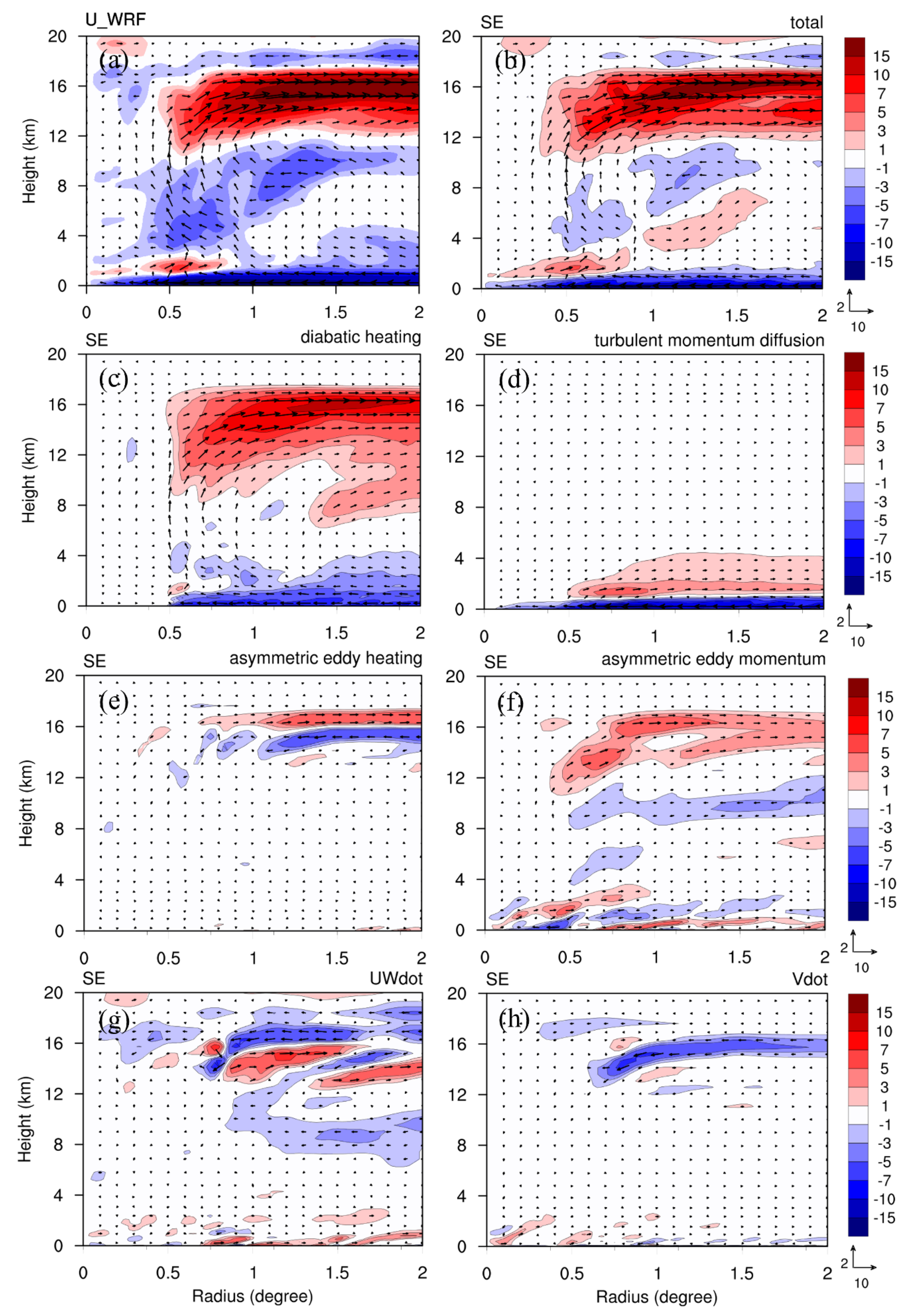
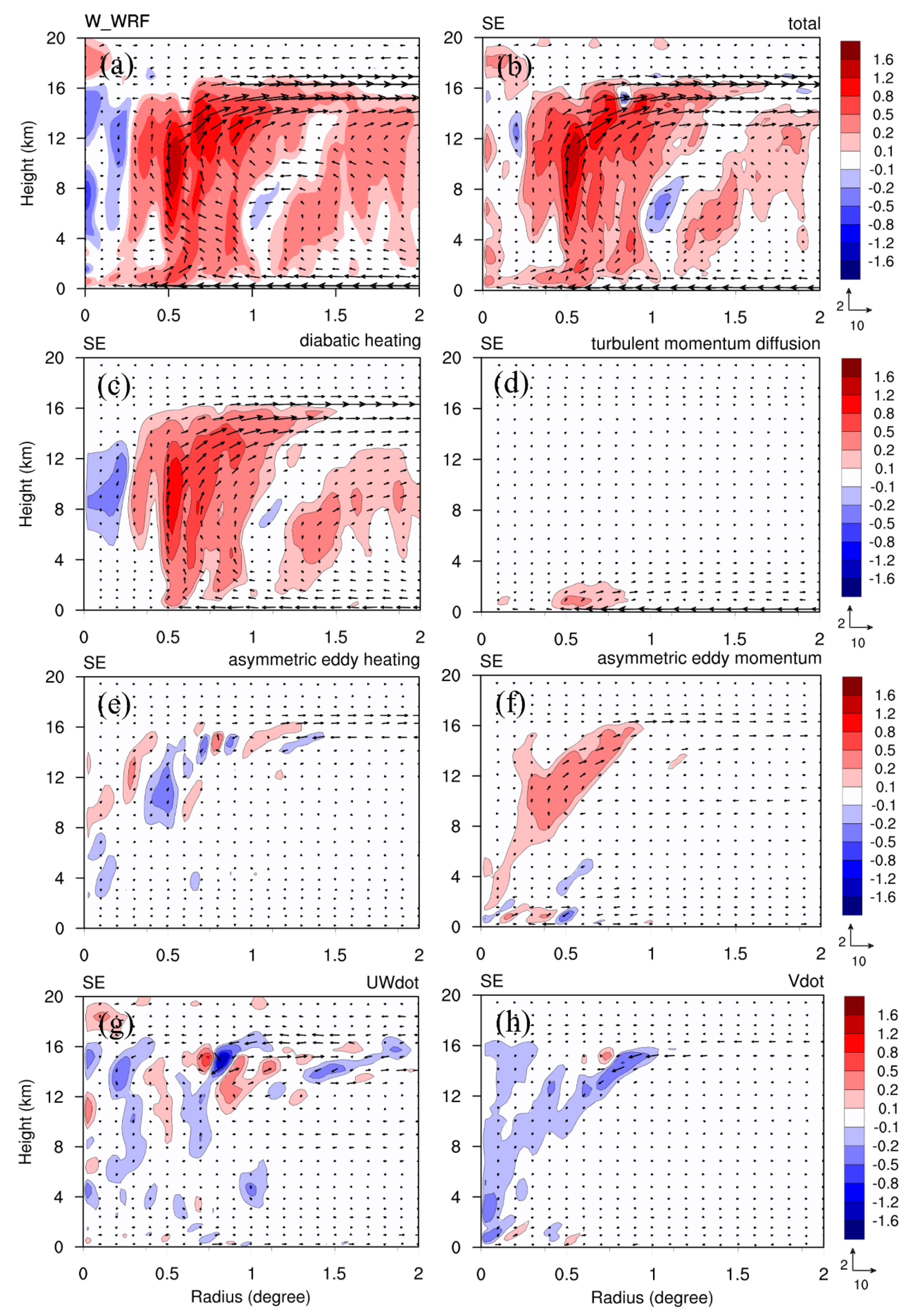
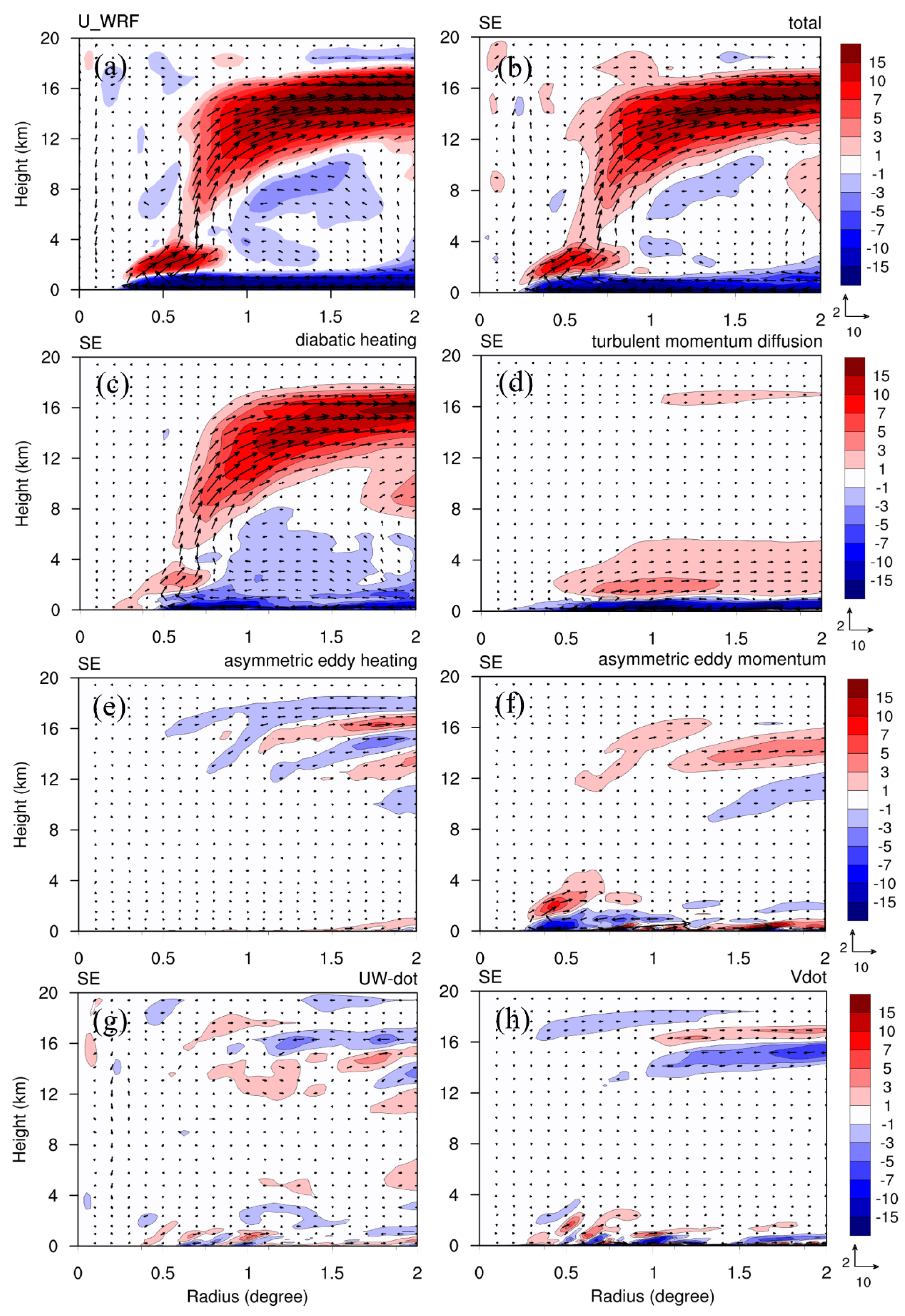
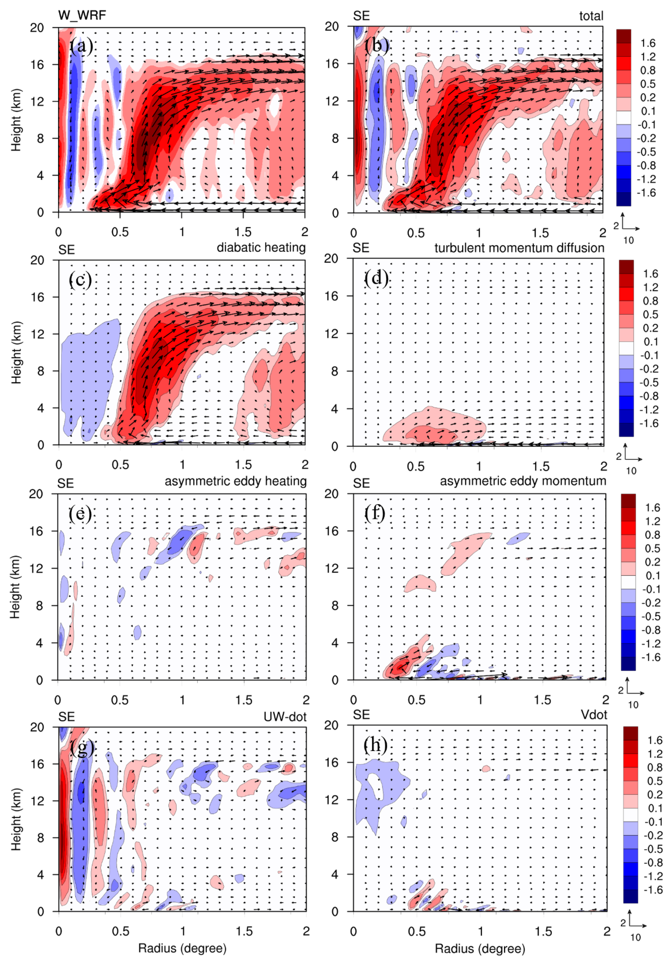
5.2. Evolutions of Secondary Circulation

We solved the extended SE equation to explore the contributions of different forcing sources to the induced transverse circulation of the primary mean vortex for Typhoon Doksuri during the RI period. More details about the formulations and limitations of the SE equation and the application of the SE solution to spinup dynamics of an intense vortex can be found in [33]. Following [33], the forcing sources involved in the unbalanced vortex include symmetric diabatic heating, asymmetric eddy momentum and heating, turbulent momentum and heat diffusion, as well as the unbalanced dynamics of the radial wind tendency equation (departing from gradient-wind balance, $\dot{U}$), the non-hydrostatic equation (departing from hydrostatic balance, $\dot{W}$), and the residue from the tangential velocity tendency equation ($\dot{V}$). The numerical domain used for solving the SE equation is 0–3 degrees in the radial with a resolution of 0.025 degree and 51 vertical levels of the vertical coordinate of the WRF model.

Figure 12 shows the radial velocity from the nonlinear simulation WRF for CTL and the radial velocity induced by the SE with total forcing sources and constituents (symmetric diabatic heating, turbulent momentum diffusion, asymmetric eddy momentum and heating, and the residual terms) at 24 h. The results show that the SE solution (Figure 12b) gives consistent radial velocity compared well with the nonlinear model results (Figure 12a), except for the underestimated upper-level outflow near 16 km height and the radial inflow in the mid-upper troposphere at 3–11 km height at a radius of 0.3–1.5 degrees. These comparisons indicate that the unbalanced SE solution may reasonably depict the developed transverse circulation of nonlinear simulation, even in the boundary layer.

The effect of diabatic heating induces most of the transverse circulation below 17 km height. The symmetric diabatic heating notably induced considerable radial inflow in the boundary layer below 4 km and prominent mid-to-upper radial outflow between 8 and 17 km height (Figure 12c). Turbulent momentum diffusion induces intense radial inflow below 1 km and some weak radial outflow above and up to 4 km (Figure 12d). Asymmetric eddy heating primarily affects upper levels, specifically between 14 and 17 km height, with coupled radial inflow and outflow below and above 16 km, respectively (Figure 12e). Conversely, the impact of asymmetric eddy momentum is slightly smaller and spans from the boundary layer to the upper troposphere (Figure 12f). The contribution of $\dot{U}$ and $\dot{W}$ to the radial velocity are mainly concentrated in the upper level above 12 km height (Figure 11g). The $\dot{V}$ has contributed to some radial outflow in the upper level at about 14 km height (Figure 12h), which may be offset by the radial inflow induced by the asymmetric eddy momentum (Figure 12f). In summary, the radial velocity at this time is mainly induced by the symmetric diabatic heating, consistent with previous studies [30,32].

Similar to Figure 12, Figure 13 shows the azimuthal-mean vertical velocity from the nonlinear simulation and induced by the SE solutions at 24 h. The SE solution with total forcing sources also effectively captures the vertical motions, but with the weaker downdraft inside of the eyewall (Figure 13a,b). The vertical updraft is mainly induced by the symmetric diabatic heating in the primary eyewall and the outer weaker eyewall (from a radius of 1.1 degrees) (Figure 13c). Turbulent momentum diffusion and asymmetric eddy momentum induced small vertical updrafts: turbulent momentum diffusion induces vertical updrafts in the boundary layer below 2 km within the eyewall (Figure 13d), while asymmetric eddy momentum induces vertical updrafts inside the eye from 8 to 16 km height (Figure 13f). Note that the contribution of asymmetric eddy momentum to vertical velocity is insignificant (Figure 13e). The contribution from the sum of $\dot{U}$ and $\dot{W}$ to the vertical velocity is mainly concentrated between 8 and 16 km height (Figure 13g), while $\dot{V}$ contributes small downward motions near the eye and upper eyewall outflow (Figure 13h).

The transverse circulation intensifies notably in the nonlinear simulation at 48 h as the RI becomes severe (Figure 14a), compared to that at 24 h (Figure 12a). At 48 h, the SE solution (Figure 14b) gives consistent radial velocity compared well with the nonlinear simulation (Figure 14a), except for the slightly underestimated radial inflow in the mid-troposphere outside the eyewall. The boundary-layer inflow and the radial upper-level outflow at 24 h are much more enhanced at 48 h, resulting from the stronger radial velocity induced by the symmetric diabatic heating (Figure 14c). The strong inflow in the upper boundary layer in the eyewall is mainly induced by the symmetric diabatic heating (Figure 14c) and the asymmetric eddy momentum (Figure 14f). In the lower boundary layer, the turbulent diffusion is a vital contributor of the intense radial inflow. Contributions from other terms remain generally consistent with those observed at 24 h. Asymmetric eddy heating primarily impacts to the radial velocity at upper levels (Figure 14e), while residual terms ($\dot{U}$, $\dot{V}$, and $\dot{W}$) minimally contribute to induced transverse circulation outside the eyewall, predominantly manifesting as weak inflow and outflow above 12 km height and within the boundary layer (Figure 14g,h).

The SE solution (Figure 15a) effectively captures the vertical updrafts in the primary eyewall and further outward outer eyewall, as well as the updrafts and downdrafts within the eye, closely following the nonlinear simulation (Figure 15a) at 48 h. In the major eyewall, vertical updrafts are primarily induced from symmetric diabatic heating, whereas within the eye, both updrafts and downdrafts are induced from the combined effects of $\dot{U}$ and $\dot{W}$ (Figure 15g). This highlights the fact that the vortex dynamics are neither in gradient balance nor in hydrostatic balance, suggesting the importance of nonhydrostatic unbalanced dynamics in the inner eyewall and eye at this stage. Turbulent momentum diffusion induces minor updrafts in the eyewall below 3 km height (Figure 15d), while contributions from asymmetric eddy heating and $\dot{V}$ to vertical velocity are negligible (Figure 15e,h). Using the SE equation to analyze different periods during typhoon intensification indicates that the SE equation can effectively quantify the contributions of different forcing components to the development of the secondary circulation and thus the vortex spinup, and the total heating source turns out to provide the most significant contribution. The momentum sources (both turbulent momentum diffusion and asymmetric eddy momentum) in general provide smaller contributions than the total heating source (all symmetric diabatic heating, turbulent heat diffusion and asymmetric eddy heating), except in the boundary layer that the induced radial inflow is more comparable or even stronger due to the turbulent diffusion in unbalanced dynamics. The symmetric diabatic heating is significant for the induced transverse circulation of the typhoon with enhanced upward motions and strong inflow and outflow, thus responsible for speeding up the vortex intensification. On the other hand, eddy temperature transport only contributes slightly, mainly at 8–18 km height. The contribution of turbulent heat diffusion to secondary circulation is also insignificant.

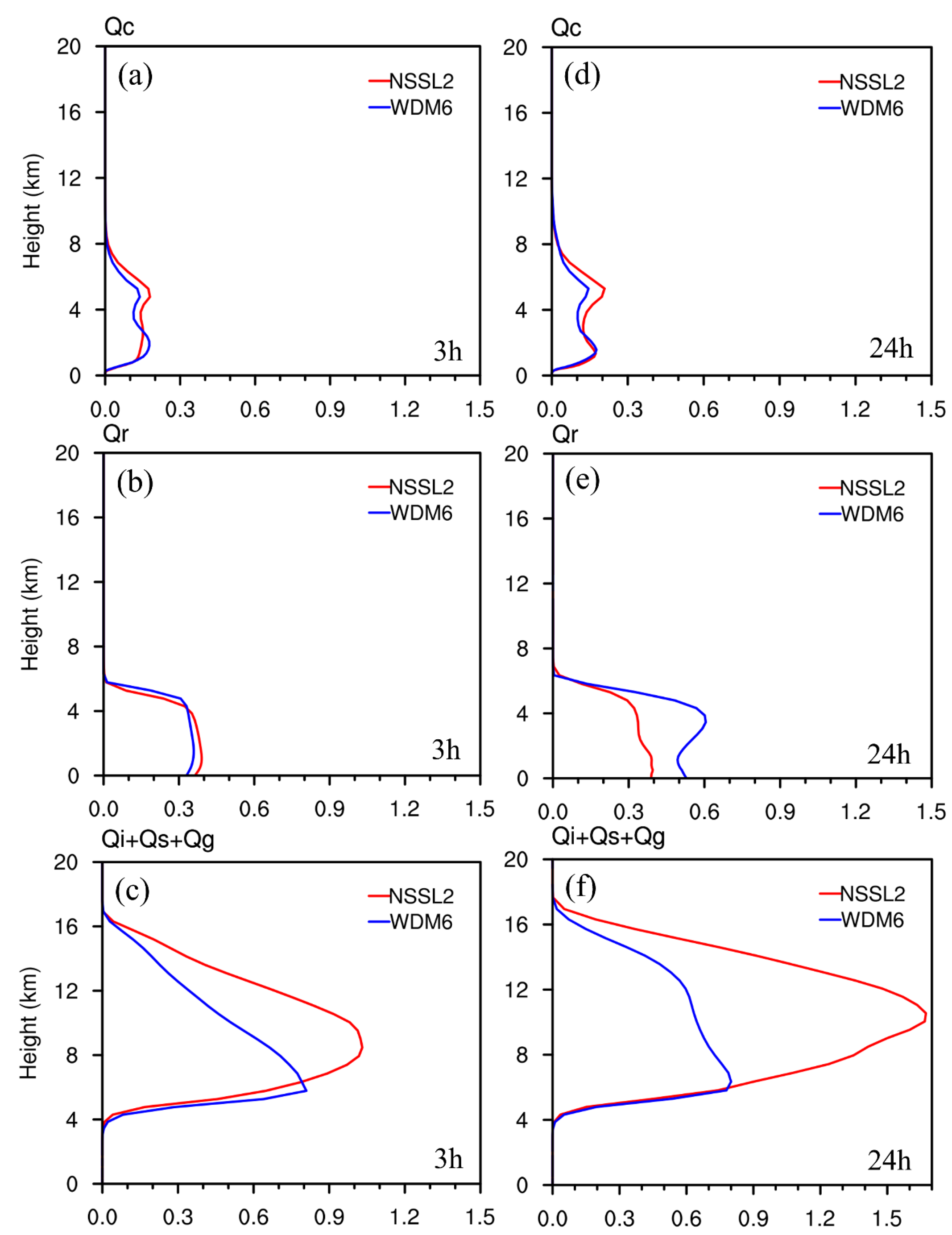
5.3. Cloud Microphysical Impacts

The combination of the GF cumulus scheme and NSSL2 microphysics scheme simulated the strongest typhoon intensity (Figure 2f) among all 15 MPSs used in this study, while the combination with the WDM6 scheme resulted in the weakest intensity (Figure 3b). Therefore, in this section, we focus on these two double-moment MPSs (NSSL2 and WDM6) to compare their influences on the prediction of Typhoon Doksuri’s intensity. This comparison aims to provide a comprehensive understanding of the cloud microphysical impacts on typhoon intensity simulation.

Figure 16 shows the contoured frequency by altitude diagrams (CFAD) for vertical velocity within a radius of 150 km from the vortex center at 3 h and 24 h for WDM6 and NSSL2. CFAD provides a statistical measure of the convection associated with a developing TC (Yuter and Houze 1995). At 3 h, when the simulated typhoon intensity is approximately 35 m s⁻¹ for both experiments, there is no significant difference in moderate updrafts in the lower and upper troposphere between the two experiments (Figure 16a,b). However, strong updrafts (w > 7 m s⁻¹) develop to higher levels for WDM6, reaching heights of 10–16 km, while for NSSL2 they remain below 10 km height. Therefore, the vertical velocity for WDM6 at this time is slightly stronger than that for NSSL2 in the upper troposphere. At 24 h, the upward motions of NSSL2 and WDM6 (Figure 16c,d) increase significantly compared to 3 h. At 24 h, the V_max for NSSL2 is about 58 m s⁻¹, much stronger than 48 m s⁻¹ for WDM6. Moderate updrafts (w < 5 m s⁻¹) are found at all levels above the boundary layer up to a 14 km height for both experiments. However, moderately strong vertical motions (5 m s⁻¹ < w < 10 m s⁻¹) develop to a higher level for WDM6 than for NSSL2, while stronger vertical updrafts (w > 10 m s⁻¹) develop to higher levels for NSSL2 than for WDM6. At 48 h, NSSL2 produces much stronger and higher updrafts than WDM6 (figures not shown). The strong updrafts are coincident with the vertical intense cloud heating as shown in Figure 6. This indicates that NSSL2 exhibits stronger upward motions that reach higher into the upper troposphere than WDM6, leading to stronger intensification.

To gain a further understanding of the differences in the cloud microphysical processes, the distributions of cloud hydrometeors were considered. Figure 17 shows the vertical profiles of averaged mixing ratios within a radius of 200 km from the typhoon center for cloud water (Q_c), rainwater (Q_r), as well as the sum of ice (Q_i), snow (Q_s), and graupel (Q_g) at 3 and 24 h for WDM6 and NSSL2. Q_c is mainly concentrated at heights of 1–6 km for both experiments (Figure 17a,d). At 24 h, Q_c for both NSSL2 and WDM6 develops at slightly higher levels but maintains the same magnitude compared to 3 h. In general, Q_c above 3 km height is slightly stronger for NSSL2 at both 3 h and 24 h. Q_r is primarily concentrated below 6 km height for both experiments, with the Q_r values being almost similar at all levels at 3 h, while it is considerably larger for WDM6 at 24 h (Figure 17d,e). At 3 h, the total mixing ratios of ice-phase hydrometeors (Q_i + Q_s + Q_g) for NSSL2 are considerably larger than those for WDM6 (Figure 17c). The peak value of the total mixing ratio (Q_i + Q_s + Q_g) is about 0.7 kg kg⁻¹ and occurs at 5 km height for WDM6, while for NSSL2, it is about 1.0 kg kg⁻¹ and occurs at a higher level of around 8 km. At 24 h, the mixing ratios for both experiments increase and develop to higher levels compared to 3 h (Figure 17f). We note that both Q_i and Q_s for NSSL2 are much larger than WDM6, while the associated Q_g is considerably smaller (figures not shown). The larger ice-phase hydrometeors for NSSL2 can be attributed to the developed higher and stronger vertical updrafts in Figure 16. The findings indicate that the mixing ratios produced by the stronger experiment (NSSL2) are larger than those of the weaker experiment (WDM6). Additionally, the convective activity in NSSL2 is greater than in WDM6, resulting in a more vigorous intensification of the typhoon. Thus, more accurately simulating the ice-phase hydrometeors is vital to the upper vortex development at the RI stage as shown for NSSL2 in Figure 16.

6. Conclusions

Typhoon Doksuri (2023) originated from an area of low pressure near the east of southeastern Luzon. The typhoon underwent RI and headed northwestward toward the northern Philippines. For the majority of its existence, the typhoon primarily moved northwestward. However, as it approached the northern part of Luzon Island, the typhoon changed mainly to a westward movement and made landfall on Bau Island, and then took a more northward track southwest of Taiwan. In this study, the WRF model was used to simulate the evolution of Typhoon Doksuri as it approached the eastern coast of the northern Philippines and moved near Taiwan, as well as to investigate its RI process over the open ocean.

Sensitivity experiments were conducted using different cloud microphysics and cumulus parameterization schemes. The results indicate that Doksuri exhibited lower sensitivity to the use of different physics parameterizations for track prediction, but greater sensitivity for intensity prediction. All the experiments well captured the observed northwestward movement in the first two days; however, they failed to capture the movement of Doksuri after the first two days when the typhoon approached the northern part of Luzon Island and crossed the Bashi Channel, regardless of the combination of physics schemes. All the experiments could capture the RI of Doksuri, but with different intensification rates and a time lag of 12 h. The combination of the GF cumulus scheme and the NSSL2 microphysics scheme was determined to be optimal (denoted by CTL) for reproducing Typhoon Doksuri.

Dynamic processes in the track changes of Doksuri were analyzed based on the CTL simulation. Regions with stronger wind speeds predominantly occurred in the north (east) of the typhoon center, which could be part of the reason why Doksuri moved westward (northwestward) when it approached (moved farther from) the northern part of the Philippines. The upward motions and diabatic heating showed greater symmetry as the typhoon approached the northern part of Luzon. As the typhoon moved farther from the northern part of the Philippines, it exhibited a counterclockwise phase rotation from northwest (at 60 h) to south (at 84 h). By using the WN-1 PV tendency budget, we found that the vertical PV advection and differential diabatic heating somewhat contributed to the typhoon’s movement after 72 h, but their effects nearly cancelled out with each other. In general, the horizontal PV advection primarily governed the PV tendency throughout most of the simulation period. The terrain sensitivity experiments showed that the track changes of CTL before and after approaching the northern part of Luzon Island and as it neared Taiwan were not largely sensitive to the whole Philippines and Taiwan terrain. When both the Philippines and Taiwan were set to plain, the typhoon, however, consistently maintained a northwestward translation most of the time.

During the RI period of Typhoon Doksuri, the latent heat flux increased steadily and became more symmetrically organized. The strong latent heat released from 24 to 48 h coincided with increased vertical velocity and diabatic heating. This indicates that strong upward motions, releasing latent heat within the inner core, could further strengthen the transverse circulation and rapidly spin up the vortex. Throughout the RI period, Doksuri experienced low VWS, which was conducive to its intensification. In this study, the extended SE equation, as used in [32], was solved to investigate the induced transverse circulation from different forcing sources for CTL at different intensification stages. The forcing sources used for the extended SE equation include mean diabatic heating, asymmetric eddy transport, turbulent diffusion, and the forcing terms associated with the unbalanced dynamics for the radial-wind equation and hydrostatic equation, accounting for agradient and nonhydrostatics, respectively, as well as the residue from the tangential velocity tendency equation. The solution of the extended SE equation agreed well with the nonlinear simulation at different stages. The results show that the transverse circulation was primarily driven by mean diabatic heating in Doksuri. Increased mean diabatic heating led to enhanced upward motions, stronger boundary-layer inflow, and upper-level outflow within the inner vortex. The intense radial inflow in the lower boundary layer, in particular, was driven mainly by turbulent momentum diffusion in response to unbalanced dynamics. Thus, the transverse circulation both above and within the boundary layer was predominantly induced by diabatic heating and turbulent friction, respectively, with negligible contributions from other forcing terms. Additionally, using the SE equation also indicated that at 48 h, $\dot{U}$ and $\dot{W}$ exerted strong impacts on vertical motions inside of the eyewall. This emphasizes the fact that the vortex dynamics of RI for this Doksuri case were neither in gradient balance nor in hydrostatic balance, suggesting the importance of nonhydrostatic unbalanced dynamics in the inner eyewall and eye at this stage.

References

1. Emanuel, K.; DesAutels, C.; Holloway, C.; Korty, R. Environmental Control of Tropical Cyclone Intensity. J. Atmos. Sci. 2004, 61, 843–858. [Google Scholar] [CrossRef]
2. Cangialosi, J.P.; Blake, E.; DeMaria, M.; Penny, A.; Latto, A.; Rappaport, E.; Tallapragada, V. Recent progress in tropical cyclone intensity forecasting at the National Hurricane Center. Weather Forecast. 2020, 35, 1913–1922. [Google Scholar] [CrossRef]
3. Gall, R.; Franklin, J.; Marks, F.; Rappaport, E.N.; Toepfer, F. The hurricane forecast improvement project. Bull. Am. Meteorol. Soc. 2013, 94, 329–343. [Google Scholar] [CrossRef]
4. Jiang, G.Q.; Xu, J.; Wei, J. A deep learning algorithm of neural network for the parameterization of typhoon-ocean feedback in typhoon forecast models. Geophys. Res. Lett. 2018, 45, 3706–3716. [Google Scholar] [CrossRef]
5. Knaff, J.A.; Sampson, C.R.; Strahl, B.R. A tropical cyclone rapid intensification prediction aid for the Joint Typhoon Warning Center’s areas of responsibility. Weather Forecast. 2020, 35, 1173–1185. [Google Scholar] [CrossRef]
6. Shi, D.; Chen, G. The implication of outflow structure for the rapid intensification of tropical cyclones under vertical wind shear. Mon. Weather Rev. 2021, 149, 4107–4127. [Google Scholar] [CrossRef]
7. Holliday, C.R.; Thompson, A.H. Climatological characteristics of rapidly intensifying typhoons. Mon. Weather Rev. 1979, 107, 1022–1034. [Google Scholar] [CrossRef]
8. Kaplan, J.; DeMaria, M. Large-scale characteristics of rapidly intensifying tropical cyclones in the North Atlantic basin. Weather Forecast. 2003, 18, 1093–1108. [Google Scholar] [CrossRef]
9. Li, X. Sensitivity of WRF simulated typhoon track and intensity over the Northwest Pacific Ocean to cumulus schemes. Sci. China Earth Sci. 2013, 56, 270–281. [Google Scholar] [CrossRef]
10. Chen, S.; Qian, Y.-K.; Peng, S. Effects of various combinations of boundary layer schemes and microphysics schemes on the track forecasts of tropical cyclones over the South China Sea. Nat. Hazards 2015, 78, 61–74. [Google Scholar] [CrossRef]
11. Islam, T.; Srivastava, P.K.; Rico-Ramirez, M.A.; Dai, Q.; Gupta, M.; Singh, S.K. Tracking a tropical cyclone through WRF–ARW simulation and sensitivity of model physics. Nat. Hazards 2015, 76, 1473–1495. [Google Scholar] [CrossRef]
12. Chandrasekar, R.; Balaji, C. Sensitivity of tropical cyclone Jal simulations to physics parameterizations. J. Earth Syst. Sci. 2012, 121, 923–946. [Google Scholar] [CrossRef]
13. Kanase, R.D.; Salvekar, P. Effect of physical parameterization schemes on track and intensity of cyclone LAILA using WRF model. Asia-Pac. J. Atmos. Sci. 2015, 51, 205–227. [Google Scholar] [CrossRef]
14. Mandal, M.; Mohanty, U.C.; Raman, S. A study on the impact of parameterization of physical processes on prediction of tropical cyclones over the Bay of Bengal with NCAR/PSU mesoscale model. Nat. Hazards 2004, 31, 391–414. [Google Scholar] [CrossRef]
15. Raju, P.; Potty, J.; Mohanty, U. Sensitivity of physical parameterizations on prediction of tropical cyclone Nargis over the Bay of Bengal using WRF model. Meteorol. Atmos. Phys. 2011, 113, 125–137. [Google Scholar] [CrossRef]
16. Srinivas, C.; Venkatesan, R.; Bhaskar Rao, D.; Hari Prasad, D. Numerical simulation of Andhra severe cyclone (2003): Model sensitivity to the boundary layer and convection parameterization. Atmos. Ocean. Mesoscale Process 2007, 164, 1465–1487. [Google Scholar] [CrossRef]
17. Chan, J.C. The physics of tropical cyclone motion. Annu. Rev. Fluid Mech. 2005, 37, 99–128. [Google Scholar] [CrossRef]
18. Tang, C.K.; Chan, J.C. Idealized simulations of the effect of Taiwan and Philippines topographies on tropical cyclone tracks. Q. J. R. Meteorol. Soc. 2014, 140, 1578–1589. [Google Scholar] [CrossRef]
19. Huang, C.-Y.; Chen, C.-A.; Chen, S.-H.; Nolan, D.S. On the upstream track deflection of tropical cyclones past a mountain range: Idealized experiments. J. Atmos. Sci. 2016, 73, 3157–3180. [Google Scholar] [CrossRef]
20. Li, D.Y.; Huang, C.Y. The influences of orography and ocean on track of Typhoon Megi (2016) past Taiwan as identified by HWRF. J. Geophys. Res. Atmos. 2018, 123, 11492–11517. [Google Scholar] [CrossRef]
21. Huang, C.-Y.; Juan, T.-C.; Kuo, H.-C.; Chen, J.-H. Track deflection of Typhoon Maria (2018) during a westbound passage offshore of northern Taiwan: Topographic influence. Mon. Weather Rev. 2020, 148, 4519–4544. [Google Scholar] [CrossRef]
22. Rostami, M.; Zeitlin, V. Evolution, propagation and interactions with topography of hurricane-like vortices in a moist-convective rotating shallow-water model. J. Fluid Mech. 2020, 902, A24. [Google Scholar] [CrossRef]
23. Chang, S.W.; Madala, R.V. Numerical simulation of the influence of sea surface temperature on translating tropical cyclones. J. Atmos. Sci. 1980, 37, 2617–2630. [Google Scholar] [CrossRef]
24. Wu, L.; Wang, B.; Braun, S.A. Impacts of air–sea interaction on tropical cyclone track and intensity. Mon. Weather Rev. 2005, 133, 3299–3314. [Google Scholar] [CrossRef]
25. Yun, K.-S.; Chan, J.C.; Ha, K.-J. Effects of SST magnitude and gradient on typhoon tracks around East Asia: Acase study for Typhoon Maemi (2003). Atmos. Res. 2012, 109, 36–51. [Google Scholar] [CrossRef]
26. Sun, J.; Oey, L.-Y. The influence of the ocean on Typhoon Nuri (2008). Mon. Weather Rev. 2015, 143, 4493–4513. [Google Scholar] [CrossRef]
27. Wu, L.; Wang, B. A potential vorticity tendency diagnostic approach for tropical cyclone motion. Mon. Weather Rev. 2000, 128, 1899–1911. [Google Scholar] [CrossRef]
28. Hsu, L.-H.; Su, S.-H.; Fovell, R.G.; Kuo, H.-C. On typhoon track deflections near the east coast of Taiwan. Mon. Weather Rev. 2018, 146, 1495–1510. [Google Scholar] [CrossRef]
29. Bui, H.H.; Smith, R.K.; Montgomery, M.T.; Peng, J. Balanced and unbalanced aspects of tropical cyclone intensification. Q. J. R. Meteorol. Soc. A J. Atmos. Sci. Appl. Meteorol. Phys. Oceanogr. 2009, 135, 1715–1731. [Google Scholar] [CrossRef]
30. Heng, J.; Wang, Y.; Zhou, W. Revisiting the balanced and unbalanced aspects of tropical cyclone intensification. J. Atmos. Sci. 2017, 74, 2575–2591. [Google Scholar] [CrossRef]
31. Montgomery, M.T.; Persing, J. Does balance dynamics well capture the secondary circulation and spinup of a simulated hurricane? J. Atmos. Sci. 2021, 78, 75–95. [Google Scholar] [CrossRef]
32. Ji, D.; Qiao, F. Does extended Sawyer–Eliassen equation effectively capture the secondary circulation of a simulated tropical cyclone? J. Atmos. Sci. 2023, 80, 871–888. [Google Scholar] [CrossRef]
33. Nguyen, T.-C.; Huang, C.-Y. Investigation on the Intensification of Supertyphoon Yutu (2018) Based on Symmetric Vortex Dynamics Using the Sawyer–Eliassen Equation. Atmosphere 2023, 14, 1683. [Google Scholar] [CrossRef]
34. Montgomery, M.T.; Smith, R.K. Paradigms for tropical cyclone intensification. Aust. Meteorol. Oceanogr. J. 2014, 64, 37–66. [Google Scholar] [CrossRef]
35. Skamarock, W.; Klemp, J.; Dudhia, J.; Gill, D.; Liu, Z.; Berner, J.; Wang, W.; Powers, J.; Duda, M.; Barker, D. A Description of the Advanced Research WRF Model Version 4.3; No. NCAR/TN556+ STR; NCAR: Boulder, CO, USA, 2021. [Google Scholar] [CrossRef]
36. Sun, J.; He, H.; Hu, X.; Wang, D.; Gao, C.; Song, J. Numerical simulations of typhoon Hagupit (2008) using WRF. Weather Forecast. 2019, 34, 999–1015. [Google Scholar] [CrossRef]
37. Park, J.; Moon, J.; Cho, W.; Cha, D.H.; Lee, M.I.; Chang, E.C.; Kim, J.; Park, S.H.; An, J. Sensitivity of Real-Time Forecast for Typhoons Around Korea to Cumulus and Cloud Microphysics Schemes. J. Geophys. Res. Atmos. 2023, 128, e2022JD036709. [Google Scholar] [CrossRef]
38. Lin, Y.-L.; Farley, R.D.; Orville, H.D. Bulk parameterization of the snow field in a cloud model. J. Appl. Meteorol. Climatol. 1983, 22, 1065–1092. [Google Scholar] [CrossRef]
39. Hong, S.-Y.; Dudhia, J.; Chen, S.-H. A revised approach to ice microphysical processes for the bulk parameterization of clouds and precipitation. Mon. Weather Rev. 2004, 132, 103–120. [Google Scholar] [CrossRef]
40. Hong, S.-Y.; Lim, J.-O.J. The WRF single-moment 6-class microphysics scheme (WSM6). Asia-Pac. J. Atmos. Sci. 2006, 42, 129–151. [Google Scholar]
41. Tao, W.K.; Wu, D.; Lang, S.; Chern, J.D.; Peters-Lidard, C.; Fridlind, A.; Matsui, T. High-resolution NU-WRF simulations of a deep convective-precipitation system during MC3E: Further improvements and comparisons between Goddard microphysics schemes and observations. J. Geophys. Res. Atmos. 2016, 121, 1278–1305. [Google Scholar] [CrossRef]
42. Thompson, G.; Field, P.R.; Rasmussen, R.M.; Hall, W.D. Explicit forecasts of winter precipitation using an improved bulk microphysics scheme. Part II: Implementation of a new snow parameterization. Mon. Weather Rev. 2008, 136, 5095–5115. [Google Scholar] [CrossRef]
43. Rogers, E.; Black, T.; Ferrier, B.; Lin, Y.; Parrish, D.; DiMego, G. National Oceanic and Atmospheric Administration Changes to the NCEP Meso Eta Analysis and Forecast System: Increase in resolution, new cloud microphysics, modified precipitation assimilation, modified 3DVAR analysis. NWS Tech. Proced. Bull. 2001, 488, 15. [Google Scholar]
44. Milbrandt, J.; Yau, M. A multimoment bulk microphysics parameterization. Part I: Analysis of the role of the spectral shape parameter. J. Atmos. Sci. 2005, 62, 3051–3064. [Google Scholar] [CrossRef]
45. Morrison, H.; Thompson, G.; Tatarskii, V. Impact of cloud microphysics on the development of trailing stratiform precipitation in a simulated squall line: Comparison of one-and two-moment schemes. Mon. Weather Rev. 2009, 137, 991–1007. [Google Scholar] [CrossRef]
46. Lin, Y.; Colle, B.A. A new bulk microphysical scheme that includes riming intensity and temperature-dependent ice characteristics. Mon. Weather Rev. 2011, 139, 1013–1035. [Google Scholar] [CrossRef]
47. Lim, K.-S.S.; Hong, S.-Y. Development of an effective double-moment cloud microphysics scheme with prognostic cloud condensation nuclei (CCN) for weather and climate models. Mon. Weather Rev. 2010, 138, 1587–1612. [Google Scholar] [CrossRef]
48. Mansell, E.R.; Ziegler, C.L.; Bruning, E.C. Simulated electrification of a small thunderstorm with two-moment bulk microphysics. J. Atmos. Sci. 2010, 67, 171–194. [Google Scholar] [CrossRef]
49. Gilmore, M.S.; Straka, J.M.; Rasmussen, E.N. Precipitation uncertainty due to variations in precipitation particle parameters within a simple microphysics scheme. Mon. Weather Rev. 2004, 132, 2610–2627. [Google Scholar] [CrossRef]
50. Morrison, H.; Milbrandt, J.A. Parameterization of cloud microphysics based on the prediction of bulk ice particle properties. Part I: Scheme description and idealized tests. J. Atmos. Sci. 2015, 72, 287–311. [Google Scholar] [CrossRef]
51. Kain, J.S. The Kain–Fritsch convective parameterization: An update. J. Appl. Meteorol. 2004, 43, 170–181. [Google Scholar] [CrossRef]
52. Grell, G.A.; Freitas, S.R. A scale and aerosol aware stochastic convective parameterization for weather and air quality modeling. Atmos. Chem. Phys. 2014, 14, 5233–5250. [Google Scholar] [CrossRef]
53. Grell, G.A.; Dévényi, D. A generalized approach to parameterizing convection combining ensemble and data assimilation techniques. Geophys. Res. Lett. 2002, 29, 38-1–38-4. [Google Scholar] [CrossRef]
54. Zhang ChunXi, Z.C.; Wang YuQing, W.Y. Projected future changes of tropical cyclone activity over the western North and South Pacific in a 20-km-mesh regional climate model. J. Clim. 2017, 30, 5923–5941. [Google Scholar] [CrossRef]
55. Hong, S.-Y.; Noh, Y.; Dudhia, J. A new vertical diffusion package with an explicit treatment of entrainment processes. Mon. Weather Rev. 2006, 134, 2318–2341. [Google Scholar] [CrossRef]
56. Dudhia, J. Numerical study of convection observed during the winter monsoon experiment using a mesoscale two-dimensional model. J. Atmos. Sci. 1989, 46, 3077–3107. [Google Scholar] [CrossRef]
57. Mlawer, E.J.; Taubman, S.J.; Brown, P.D.; Iacono, M.J.; Clough, S.A. Radiative transfer for inhomogeneous atmospheres: RRTM, a validated correlated-k model for the longwave. J. Geophys. Res. Atmos. 1997, 102, 16663–16682. [Google Scholar] [CrossRef]
58. Nguyen, T.-C.; Huang, C.-Y. A comparative modeling study of Supertyphoons Mangkhut and Yutu (2018) past the Philippines with ocean-coupled HWRF. Atmosphere 2021, 12, 1055. [Google Scholar] [CrossRef]
59. Chang, C.-C.; Wu, C.-C. On the processes leading to the rapid intensification of Typhoon Megi (2010). J. Atmos. Sci. 2017, 74, 1169–1200. [Google Scholar] [CrossRef]
Figure 1. The two nested domains of the WRF model for Doksuri during the simulation time. The outermost box and white box denote the outer and the inner domains, respectively. The black line with color dots at intervals of 12 h indicates the best track from the IBTrACS from 1200 UTC 23 July to 1200 UTC 28 July 2023. The color of the dots represents different typhoon intensity categories according to the Saffir–Simpson scale for Typhoon Doksuri (2023).
Atmosphere 15 01105 g001
Figure 2. Tracks of Typhoon Doksuri including the best track data from IBTrACS (solid black line) and JMA (dashed black line) as well as simulated tracks from sensitivity experiments that combined the CPSs (a) KF, (b) GF, (c) GD, and (d) New Tiedtke with different MPSs (solid colored lines) during the period from 1200 UTC 23 July to 1200 UTC 28 July 2023 (0 to 120 forecast hours). The circle symbols indicate the time every 24 h. (eh) as in (ad), respectively, but for the 10 m maximum wind speed (Vmax, m s−1). The blue, green, magenta, yellow, red, and cyan lines denote the cloud microphysics schemes Lin, WSM6, Goddard, Thompson, NSSL2, and P3, respectively.
Atmosphere 15 01105 g002
Figure 3. (a) Track of Typhoon Doksuri including the best track data from IBTrACS (solid black line) and JMA (dashed black line) as well as simulated tracks from the sensitivity experiments using the GF cumulus schemes combined with nine different MPSs (solid colored lines) during the period from 1200 UTC 23 July to 1200 UTC 28 July 2023 (0 to 120 forecast hours). The circle symbols indicate the time every 24 h. The 9 different MPSs are listed in Table 1. (b) as in (a) but for the 10 m maximum wind speed (Vmax, m s−1). (c) as in (a) but for the track error (km) for all the sensitivity experiments combining the GF cumulus scheme with the fifteen different MPSs, as noted in Table 1.
Atmosphere 15 01105 g003
Figure 4. Accumulated hourly precipitation (mm) from GSMaP in (a) 12 h (from 0000 UTC to 0059 UTC 24 July, (b) 24 h (from 1200 UTC to 1259 UTC 24 July), (c) 36 h (from 0000 UTC to 0059 UTC 25 July), and (d) 48 h (from 1200 UTC to 1259 UTC 25 July). (eh) as in (ad), respectively, but for simulated rainfall (mm) for CTL.
Atmosphere 15 01105 g004
Figure 5. The simulated horizontal wind speed (shaded colors, m s−1) averaged in 1–8 km height for CTL at (a) 36 h, (b) 48 h, (c) 60 h, and (d) 72 h. (eh) as in (ad) respectively, but for vertical velocity (colors shaded, m s−1). The vector shows the simulated horizontal wind averaged in 1–8 km height.
Atmosphere 15 01105 g005
Figure 6. Hovmöller plots of (a) horizontal wind speed (m s−1), (b) vertical velocity (m s−1), and (c) diabatic heating (K h−1) averaged in 1–8 km height and radii of 0.5°–1.5° concerning azimuth for Doksuri.
Atmosphere 15 01105 g006
Figure 7. Time evolution of the translation velocity (vectors, m s−1) induced by different PV budget terms, including differential diabatic heating (HDIA), vertical PV advection (VADV), horizontal PV advection (HADV), and the sum of the former three terms (SUM), during the forecast time of 120 h for CTL.
Atmosphere 15 01105 g007
Figure 8. Simulated tracks for CTL (red line), NoTW (blue line), NoPhi (green line), NoPhi-TW (magenta line), and the best track from IBTrACS (black line). The simulated time was from 1200 UTC 23 July to 1200 UTC 28 July 2023. The circle symbols indicate the time every 24 h.
Atmosphere 15 01105 g008
Figure 9. As in Figure 7 but for (a) NoTW and (b) NoPhi.
Atmosphere 15 01105 g009
Figure 10. LHF (shaded colors, W m−2) for CTL at (a) 3 h, (b) 12 h, (c) 18 h, (d) 24 h, (e) 36 h, and (f) 48 h. Solid blue circles mark the 100 and 200 km radii from the typhoon center. The vector at the typhoon center denotes the VWS averaged within the radius of 0–800 km. The number in the top-right inset of each panel denotes the magnitude of VWS.
Atmosphere 15 01105 g010
Figure 11. Azimuthal-mean diabatic heating (shaded colors, K h−1) and tangential wind (contours, at intervals of 5 m s−1) for CTL at (a) 3 h, (b) 12 h, (c) 18 h, (d) 24 h, (e) 36 h, and (f) 48 h.
Atmosphere 15 01105 g011
Figure 12. Azimuthal-mean radial velocity (shaded colors, m s−1) at 24 h from (a) the nonlinear simulation, (b) the SE solution with the total sources, (c) as in (b) but with symmetric diabatic heating only, (d) as in (b) but with turbulent momentum diffusion only, (e) as in (b) but with asymmetric eddy heating only, (f) as in (b) but with asymmetric eddy momentum only, (g) as in (b) but with U ˙ and W ˙ only, (h) as in (b) but with V ˙ only. The wind vectors (m s−1) induced by the total forcing sources overlapped in each panel indicate the radial and vertical wind components (m s−1) with their reference vectors given at the lower right corner.
Atmosphere 15 01105 g012
Figure 13. As in Figure 12 but for vertical velocity (m s−1) at 24 h for (a) the nonlinear simulation, (b) the SE solution with the total sources, (c) as in (b) but with symmetric diabatic heating only, (d) as in (b) but with turbulent momentum diffusion only, (e) as in (b) but with asymmetric eddy heating only, (f) as in (b) but with asymmetric eddy momentum only, (g) as in (b) but with U ˙ and W ˙ only, (h) as in (b) but with V ˙ only.
Atmosphere 15 01105 g013
Figure 14. As in Figure 12 but at 48 h for (a) the nonlinear simulation, (b) the SE solution with the total sources, (c) as in (b) but with symmetric diabatic heating only, (d) as in (b) but with turbulent momentum diffusion only, (e) as in (b) but with asymmetric eddy heating only, (f) as in (b) but with asymmetric eddy momentum only, (g) as in (b) but with U ˙ and W ˙ only, (h) as in (b) but with V ˙ only.
Atmosphere 15 01105 g014
Figure 15. As in Figure 13 but for vertical velocity (m s−1) at 48 h for (a) the nonlinear simulation, (b) the SE solution with the total sources, (c) as in (b) but with symmetric diabatic heating only, (d) as in (b) but with turbulent momentum diffusion only, (e) as in (b) but with asymmetric eddy heating only, (f) as in (b) but with asymmetric eddy momentum only, (g) as in (b) but with U ˙ and W ˙ only, (h) as in (b) but with V ˙ only.
Atmosphere 15 01105 g015
Figure 16. Contoured frequency by altitude diagrams (CFAD, %) of vertical velocity within a radius of 150 km from the typhoon center at 3 h for (a) WDM6 and (b) NSSL2. (c,d) as in (a,b), respectively, but at 24 h.
Atmosphere 15 01105 g016
Figure 17. Vertical profiles of hydrometeors (10−3 kg kg−1) averaged in a 200 km radius of the typhoon center for (a) cloud water mixing ratio; (b) rainwater mixing ratio; (c) total of ice mixing ratio, snow mixing ratio, and graupel mixing ratio at 3 h. (df) as in (ac), respectively, but at 24 h.
Atmosphere 15 01105 g017