Decreases in Mercury Wet Deposition over the United States during 2004–2010: Roles of Domestic and Global Background Emission Reductions

Abstract
:1. Introduction


| Period | Trends (% yr−1) | Reference | ||||
|---|---|---|---|---|---|---|
| Hg concentrations in precipitation over North America | ||||||
| Northeast | Midwest | Southeast | West | |||
| 1998–2005 | −1.7 ± 0.51a | −3.5 ± 0.74 | 0.01 ± 0.71 | 24 | ||
| 1996–2005 | −2.1 ± 0.88 b | −1.8 ± 0.28 | −1.3 ± 0.30 | −1.4 ± 0.42 | 25 | |
| 2002–2008 | 0.84 ± 2.9 b | −2.0 ± 3.8 | 26 | |||
| 2004–2010 | −4.1 ± 0.49 a | −2.7 ± 0.68 | −0.53 ± 0.59 | 2.6 ± 1.5 | This study | |
| Atmospheric Hg concentrations | ||||||
| 1995–2005 | Canada | −1.3 ± 1.9 | 33 | |||
| 1996–2009 | Mace Head, Ireland | −1.4 | 34 | |||
| Cape Point | −2.7 | |||||
| 1990–2009 | North Atlantic | −2.5 ± 0.54 | 35 | |||
| South Atlantic | −1.9 ± 0.91 | |||||
| 2000–2009 | Temperate Canada | −1.9 ± 0.3 | 36 | |||
2. Observations and Model
 ). We divide the difference by six because we assume that the change occurs over the six years elapsed between 2004 and 2010.
3. Results and Discussion
3.1. Seasonal and Interannual Variability in Hg Wet Deposition

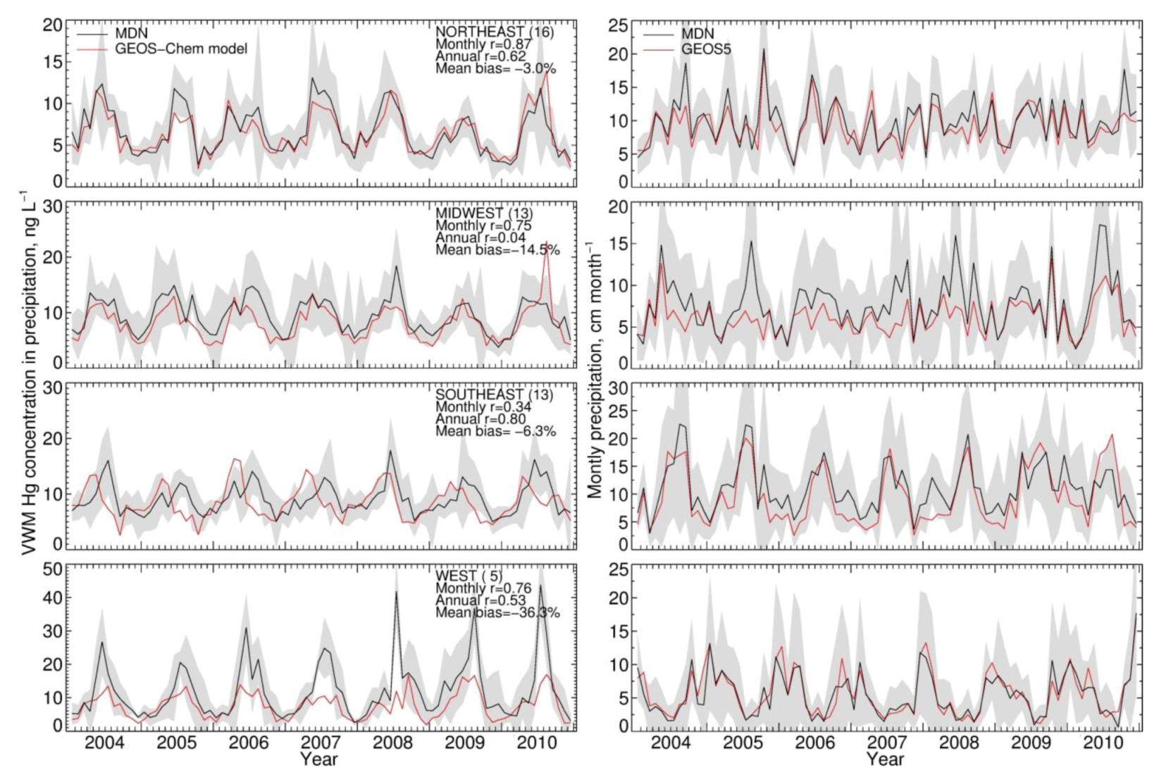
 ) varying from 20 to 40%. The coefficients of variance (ratios of standard deviation to the mean) are 12% (Northeast), 8% (Midwest), 5% (Southeast) and 12% (West). The MDN observed precipitation amounts also have significant interannual variability, with coefficients of variance of 5.0% (Northeast), 7% (Midwest), 12% (Southeast) and 20% (West). Although Hg concentrations in different years have similar seasonal patterns, the peak month and degree of seasonality can vary. For example, the West region displays much higher concentrations in August in 2008 and 2010 relative to other years. Over the Midwest, elevated Hg concentrations are measured during August 2006, 2008 and 2009, because of the relatively lower precipitation amount in these months, while the peak occurs earlier in other years. Lower Hg concentrations are observed during the summer of 2009 compared with multi-year mean in the Northeast and Midwest. The BASE simulation generally captures these features and has r values for observed and modeled annual VWM Hg concentrations of 0.54 (Northeast), 0.26 (Midwest), 0.73 (Southeast) and 0.29 (West). However, we find that the model tends to be on the high side of observations for the last three years and on the low side for the first three years, especially in the Northeast and Midwest. As we will show below, this indicates a trend in observed VWM Hg concentrations not captured by this BASE model simulation with constant anthropogenic emissions.
| Region | Number of Sites | VWM Hg Concentrations in Precipitation | Precipitation Depth (Observed) | ||||
|---|---|---|---|---|---|---|---|
| Model Subtraction | Direct Regression | ||||||
| % yr−1 | ns a | % yr−1 | ns | % yr−1 | ns | ||
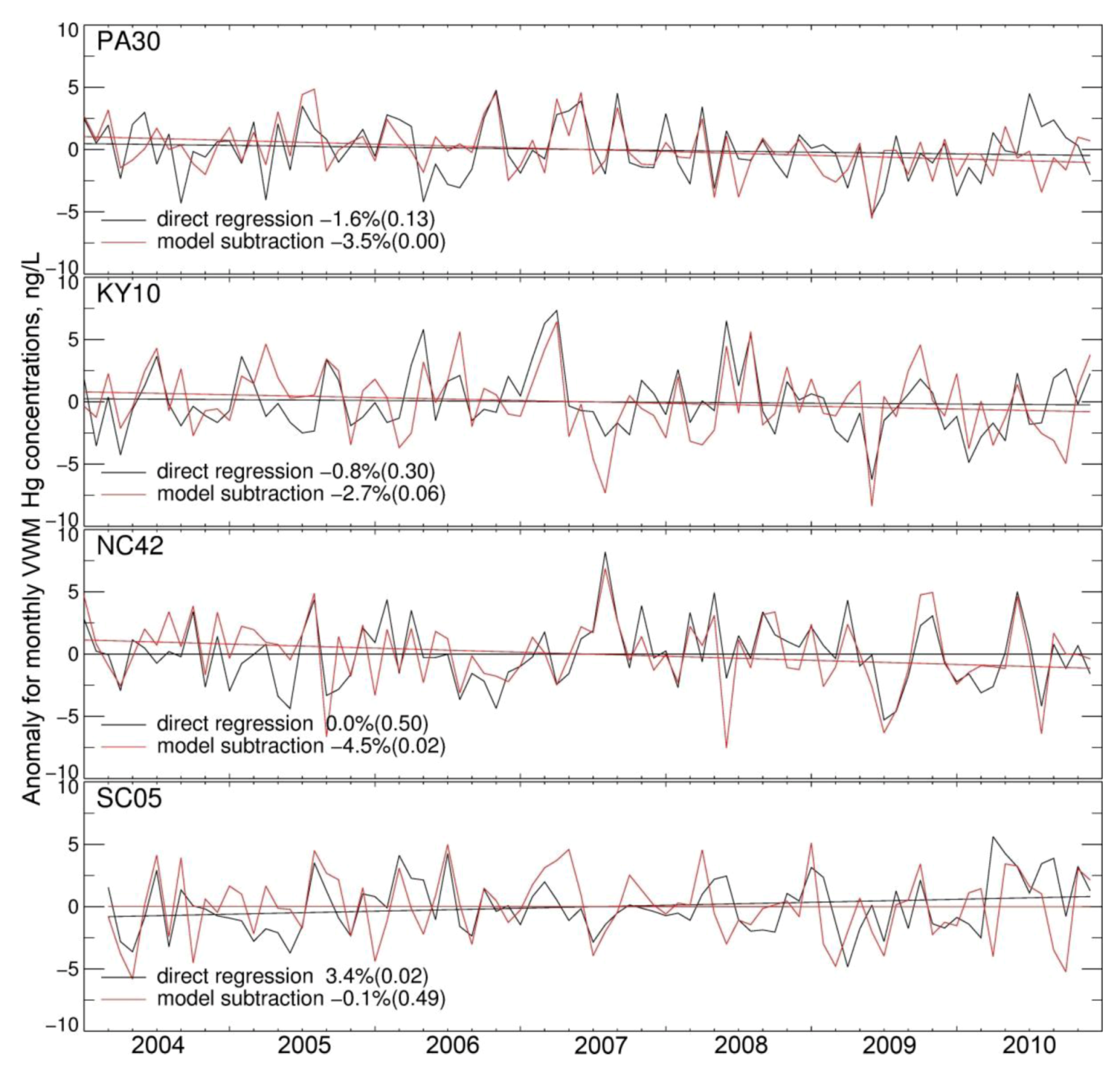
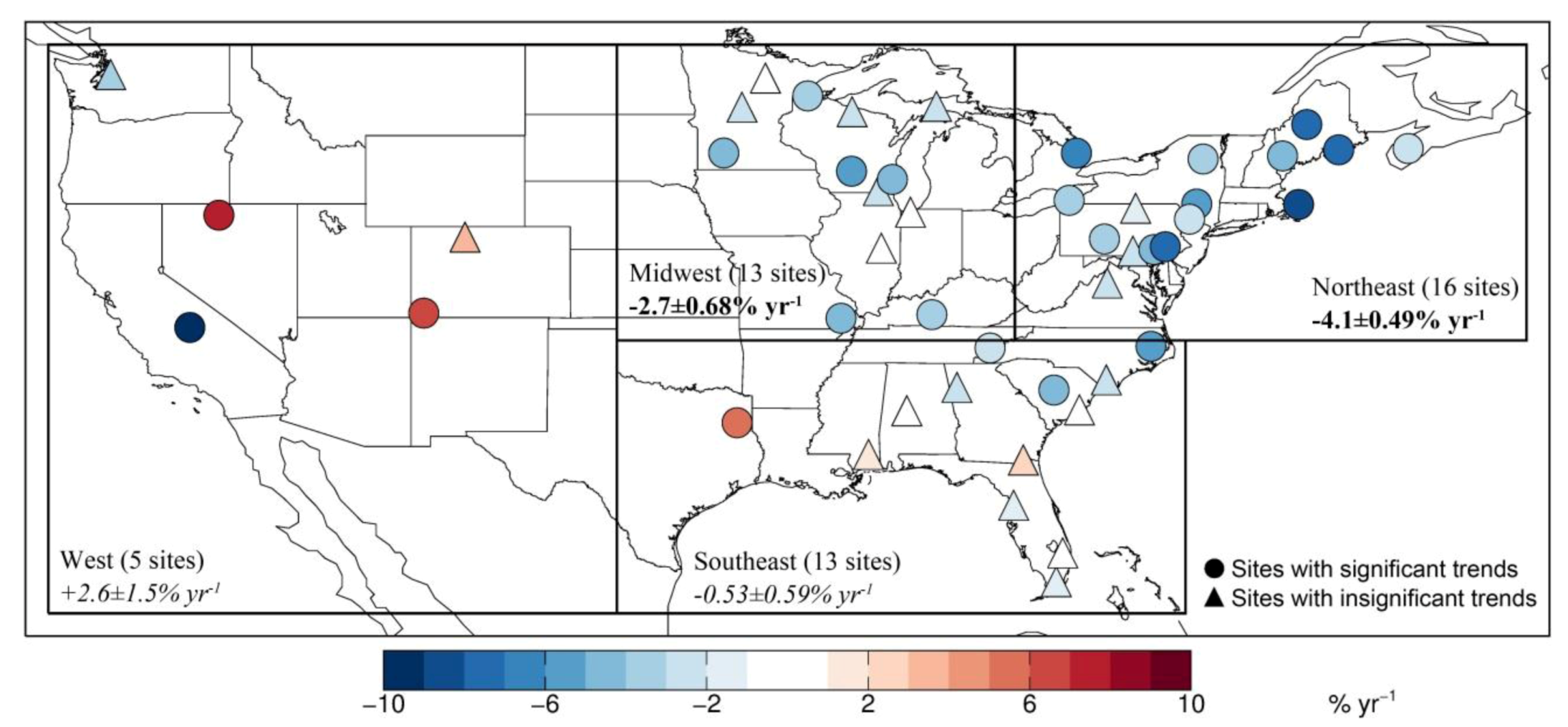
| NORTHEAST | 16 | −4.1 ± 0.49 | 13 | −3.8 ± 0.50 | 9 | +0.089 ± 0.26 | 3 |
| MIDWEST | 13 | −2.7 ± 0.68 | 6 | −2.0 ± 0.64 | 4 | +0.69 ± 0.38 | 2 |
| SOUTHEAST | 13 | −0.53 ± 0.59 | 4 | −0.36 ± 0.54 | 3 | −0.35 ± 0.32 | 6 |
| WEST | 5 | +2.6 ± 1.5 | 3 | +4.0 ± 1.5 | 3 | +1.8 ± 0.68 | 1 |
3.2. Trend in Hg Precipitation Concentrations for 2004–2010


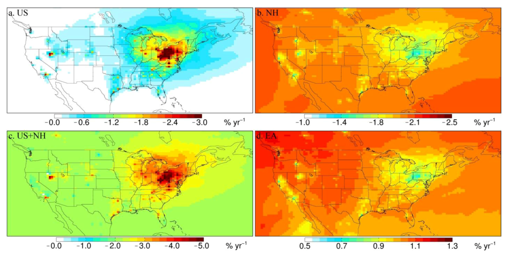
3.3. Attribution of Observed Trends

| Observations | Model Scenarios | |||||
|---|---|---|---|---|---|---|
| Region | n | USa | NHb | US+NH | EAc | |
| % yr−1 | % yr−1 | % yr−1 | % yr−1 | % yr−1 | ||
| NORTHEAST | 16 | −4.1 ± 0.49d | −2.4 ± 0.51 | −1.7 ± 0.10 | −4.1 ± 0.52 | 0.84 ± 0.048 |
| MIDWEST | 13 | −2.7 ± 0.68 | −1.4 ± 0.38 | −1.7 ± 0.47 | −3.1 ± 0.60 | 0.89 ± 0.22 |
| SOUTHEAST | 13 | −0.53 ± 0.59 | −0.55 ± 0.10 | −1.9 ± 0.18 | −2.5 ± 0.21 | 0.92 ± 0.086 |
| WEST | 5 | +2.6 ± 1.5 | +0.068 ± 0.19 | −1.9 ± 0.80 | −1.8 ± 0.82 | 1.0 ± 0.41 |
4. Conclusions
Acknowledgments
Conflict of Interest
References and Notes
- The Original List of Hazardous Air Pollutants. Available online: http://www.epa.gov/ttn/atw/188polls.html (accessed on 13 March 2013).
- Mason, R.A. Mercury Emissions from Natural Processes and their Importance in the Global Mercury Cycle. In Mercury Fate and Transport in the Global Atmosphere: Emissions, Measurements and Models; Pirrone, N., Mason, R.A., Eds.; Springer: Dordrecht, The Netherlands, 2009; pp. 173–191. [Google Scholar]
- Streets, D.G.; Devane, M.K.; Lu, Z.; Bond, T.C.; Sunderland, E.M.; Jacob, D.J. All-time releases of mercury to the atmosphere from human activities. Environ. Sci. Technol. 2011, 45, 10485–10491. [Google Scholar]
- Pirrone, N.; Cinnirella, S.; Feng, X.; Finkelman, R.B.; Friedli, H.R.; Learner, J.; Mason, R.; Mukherjee, A.B.; Stracher, G.; Streets, D.G.; Telmer, K. Global mercury emissions to the atmosphere from natural and anthropogenic sources. In Mercury Fate and Transport in the Global Atmosphere: Emissions, Measurements and Models; Pirrone, N., Mason, R.A., Eds.; Springer: Dordrecht, The Netherlands, 2009; pp. 3–50. [Google Scholar]
- Selin, N.E. Global biogeochemical cycling of mercury: A review. Annu. Rev. Environ. Resour. 2009, 34, 43–63. [Google Scholar] [CrossRef]
- Holmes, C.D.; Jacob, D.J.; Yang, X. Global lifetime of elemental mercury against oxidation by atomic bromine in the free troposphere. Geophys. Res. Lett. 2009, 33, L20808. [Google Scholar] [CrossRef]
- Clarkson, T.W. The three modern faces of mercury. Environ. Health Perspect. 2002, 110, 11–23. [Google Scholar] [CrossRef]
- Mergler, D.; Anderson, H.A.; Chan, L.H.M.; Mahaffey, K.R.; Murray, M.; Sakamoto, M.; Stern, A.H. Methylmercury exposure and health effects in humans: A worldwide concern. Ambio 2007, 36, 3–11. [Google Scholar] [CrossRef]
- Houyoux, M.; Strum, M. Memorandum: Emissions Overview: Hazardous Air Pollutants in Support of the Final Mercury and Air Toxics Standard; EPA-454/R-11-014; Emission Inventory and Analysis Group Air Quality Assessment Division: Research Triangle Park, NC, USA, 2011. [Google Scholar]
- Seigneur, C.; Vijayaraghavan, K.; Lohman, K.; Karamchandani, P.; Scott, C. Global source attribution for mercury deposition in the United States. Environ. Sci. Technol. 2004, 38, 555–569. [Google Scholar] [CrossRef]
- Selin, N.E.; Jacob, D.J. Seasonal and spatial patterns of mercury wet deposition in the United States: Constraints on the contribution from North American anthropogenic sources. Atmos. Environ. 2008, 42, 5193–5204. [Google Scholar] [CrossRef]
- Zhang, Y.; Jaeglé, L.; van Donkelaar, A.; Martin, R.V.; Holmes, C.D.; Amos, H.M.; Wang, Q.; Talbot, R.; Artz, R.; Brooks, S.; et al. Nested-grid simulation of mercury over North America. Atmos. Chem. Phys. 2012, 12, 6095–6111. [Google Scholar] [CrossRef]
- Edgerton, E.S.; Hartsell, B.E.; Jansen, J.J. Mercury speciation in coal-fired power plant plumes observed at three surface sites in the southeastern US. Environ. Sci. Technol. 2006, 40, 4563–4570. [Google Scholar] [CrossRef]
- Weiss-Penzias, P.S.; Gustin, M.S.; Lyman, S.N. Sources of gaseous oxidized mercury and mercury dry deposition at two southeastern U.S. sites. Atmos. Environ. 2011, 45, 4569–4579. [Google Scholar] [CrossRef]
- Toxics Release Inventory. Available online: http://www.epa.gov/tri/ (accessed on 13 March 2013).
- National Toxics Inventory. Available online: http://epa.gov/air/data/netemis.html (accessed on 13 March 2013).
- National Emission Inventory. Available online: http://www.epa.gov/ttn/chief/net/2008inventory.html (accessed on 13 March 2013).
- Solid Waste Combustion Rule. Available online: http://www.epa.gov/airtoxics/129/gil2.pdf (accessed on 13 March 2013).
- Clean Air Mercury Rule. Available online: http://www.epa.gov/camr/ (accessed on 13 March 2013).
- Information Collection Request. Available online: http://www.epa.gov/ttn/atw/utility/utilitypg.html (accessed on 13 March 2013).
- Mercury and Air Toxics Standard. Available online: http://www.epa.gov/mats (accessed on 13 March 2013).
- Integrated Planning Model. Available online: http://www.epa.gov/airmarkets/progsregs/epa-ipm/index.html (accessed on 13 March 2013).
- USEPA, Emissions Inventory and Emissions Processing for the Clean Air Mercury Rule (CAMR); Office of Air Quality Planning and Standards Emissions, Monitoring and Analysis Division: Research Triangle Park, NC, USA, 2005.
- Butler, T.J.; Cohen, M.D.; Vermeylen, F.M.; Likens, G.E.; Schmeltz, D.; Artz, R.S. Regional precipitation mercury trends in the eastern USA, 1998–2005: Declines in the Northeast and Midwest, no trend in the Southeast. Atmos. Environ. 2008, 42, 1582–1592. [Google Scholar] [CrossRef]
- Prestbo, E.M.; Gay, D.A. Wet deposition of mercury in the US and Canada, 1996–2005: Results and analysis of the NADP mercury deposition network (MDN). Atmos. Environ. 2009, 43, 4223–4233. [Google Scholar] [CrossRef]
- Risch, M.R.; Gay, D.A.; Fowler, K.K.; Keeler, G.J.; Backus, S.M.; Blanchard, P.; Barres, J.A.; Dvonch, J.T. Spatial patterns and temporal trends in mercury concentrations, precipitation depths, and mercury wet deposition in the North American Great Lakes region, 2002–2008. Environ. Pollut. 2012, 161, 261–271. [Google Scholar] [CrossRef]
- Gratz, L.E.; Keeler, G.J.; Miller, E.K. Long-term relationships between mercury wet deposition and meteorology. Atmos. Environ. 2009, 43, 6218–6229. [Google Scholar] [CrossRef]
- Vijayaraghavan, K.; Stoeckenius, T.; Ma, L.; Yarwood, G.; Morris, R.; Levin, L. Analysis of Temporal Trends in Mercury Emissions and Deposition in Florida. In Proceedings of the 10th International Conference on Mercury as Global Pollutant, Halifax, NS, Canada, August 2011.
- Landis, M.S.; Vette, A.F.; Keeler, G.J. Atmospheric mercury in the Lake Michigan Basin: influence of the Chicago/Gary urban area. Environ. Sci. Technol. 2002, 36, 4508–4517. [Google Scholar] [CrossRef]
- Wu, Y.; Wang, S.; Streets, D.G.; Hao, J.; Chan, M.; Jiang, J. Trends in Anthropogenic Mercury Emissions in China from 1995 to 2003. Environ. Sci. Technol. 2006, 40, 5312–5318. [Google Scholar] [CrossRef]
- Streets, D.G.; Zhang, Q.; Wu, Y. Projections of Global Mercury Emissions in 2050. Environ. Sci. Technol. 2009, 43, 2983–2988. [Google Scholar] [CrossRef]
- Tian, H.; Wang, Y.; Xue, Z.; Qu, Y.; Chai, F.; Hao, J. Atmospheric emissions estimation of Hg, As, and Se from coal-fired power plants in China, 2007. Sci. Total Environ. 2011, 409, 3078–3081. [Google Scholar] [CrossRef]
- Temme, C.; Blanchard, P.; Steffen, A.; Banic, C.; Beauchamp, S.; Poissant, L.; Tordon, R.; Wiens, B. Trend, seasonal and multivariate analysis study of total gaseous mercury data from the Canadian atmospheric mercury measurement network (CAMNet). Atmos. Environ. 2007, 41, 5423–5441. [Google Scholar] [CrossRef]
- Cole, A.S.; Steffen, A.; Pfaffhuber, K.A.; Berg, T.; Pilote, M.; Poissant, L.; Tordon, R.; Hung, H. Ten-year trends of atmospheric mercury in the high Arctic compared to Canadian sub-Arctic and mid-latitude sites. Atmos. Chem. Phys. 2013, 13, 1535–1545. [Google Scholar] [CrossRef] [Green Version]
- Slemr, F.; Brunke, E.G.; Ebinghaus, R.; Kuss, J. Worldwide trend of atmospheric mercury since 1995. Atmos. Chem. Phys. 2011, 11, 4779–4787. [Google Scholar] [CrossRef]
- Soerensen, A.L.; Jacob, D.J.; Streets, D.G.; Witt, M.L.I.; Ebinghaus, R.; Mason, R.P.; Andersson, M.; Sunderland, E.M. Multi-decadal decline of mercury in the North Atlantic atmosphere explained by changing subsurface seawater concentrations. Geophys. Res. Lett. 2012, 39, L21810. [Google Scholar]
- National Atmospheric Deposition Program, Mercury Deposition Network Information. Available online: http://nadp.sws.uiuc.edu/mdn/ (accessed on 13 March 2013).
- Bey, I.; Jacob, D.J.; Yantosca, R.M.; Logan, J.A.; Field, B.D.; Fiore, A. M.; Li, Q.B.; Liu, H.G.Y.; Mickley, L.J.; Schultz, M.G. Global modeling of tropospheric chemistry with assimilated meteorology: Model description and evaluation. J. Geophys. Res.-Atmos. 2001, 106, 23073–23095. [Google Scholar] [CrossRef]
- Selin, N.E.; Jacob, D.J.; Park, R.J.; Yantosca, R.M.; Strode, S.; Jaegle, L.; Jaffe, D. Chemical cycling and deposition of atmospheric mercury: Global constraints from observations. J. Geophys. Res. 2007, 112, D02308. [Google Scholar]
- Holmes, C.D.; Jacob, D.J.; Corbitt, E.S.; Mao, J.; Yang, X.; Talbot, R.; Slemr, F. Global atmospheric model for mercury including oxidation by bromine atoms. Atmos. Chem. Phys. 2010, 10, 12037–12057. [Google Scholar] [CrossRef]
- Amos, H.M.; Jacob, D.J.; Holmes, C.D.; Fisher, J.A.; Wang, Q.; Yantosca, R.M.; Corbitt, E.S.; Galarneau, E.; Rutter, A.P.; Gustin, M.S.; et al. Gas-particle partitioning of atmospheric Hg(II) and its effect on global mercury deposition. Atmos. Chem. Phys. 2012, 12, 591–603. [Google Scholar] [CrossRef]
- Donohoue, D.L.; Bauer, D.; Cossairt, B.; Hynes, A.J. Temperature and pressure dependent rate coefficients for the reaction of Hg with Br and the reaction of Br with Br: A pulsed laser photolysis-pulsed laser induced fluorescence study. J. Phys. Chem. A 2006, 110, 6623–6632. [Google Scholar]
- Goodsite, M.E.; Plane, J.M.C.; Skov, H. A theoretical study of the oxidation of Hg0 to HgBr2 in the troposphere. Environ. Sci. Technol. 2004, 38, 1772–1776. [Google Scholar] [CrossRef]
- Balabanov, N.B.; Shepler, B.C.; Peterson, K.A. Accurate global potential energy surface and reaction dynamics for the ground state of HgBr2. J. Phys. Chem. A 2005, 109, 8765–8773. [Google Scholar]
- Pacyna, E.G.; Pacyna, J.M.; Sundseth, K.; Munthe, J.; KinNHom, K.; Wilson, S.; Steenhuisen, F.; Maxson, P. Global emission of mercury to the atmosphere from anthropogenic sources in 2005 and projections to 2020. Atmos. Environ. 2010, 44, 2487–2499. [Google Scholar] [CrossRef]
- National Pollutant Release Inventory. Available online: http://www.ec.gc.ca/inrp-npri/ (accessed on 13 March 2013).
- Soerensen, A.L.; Sunderland, E.M.; Holmes, C.D.; Jacob, D.J.; Yantosca, R.M.; Skov, H.; Christensen, J.H.; Strode, S.A.; Mason, R.P. An Improved Global Model for Air-Sea Exchange of Mercury: High Concentrations over the North Atlantic. Environ. Sci. Technol. 2010, 44, 8574–8580. [Google Scholar]
- Liu, H.; Jacob, D.; Bey, I.; Yantosca, R.M. Constraints from Pb210 and Be7 on wet deposition and transport in a global three-dimensional chemical tracer model driven by assimilated meteorological fields. J. Geophys. Res. 2001, 106, 12109–12128. [Google Scholar]
- Wang, Q.; Jacob, D.J.; Fisher, J.A.; Mao, J.; Leibensperger, E.M.; Carouge, C.C.; Le Sager, P.; Kondo, Y.; Jimenez, J.L.; Cubison, M.J.; Doherty, S.J. Sources of carbonaceous aerosols and deposited black carbon in the Arctic in winter-spring: implications for radiative forcing. Atmos. Chem. Phys. 2011, 11, 12453–12473. [Google Scholar]
- Wesely, M.L. Parameterization of surface resistances to gaseous dry deposition in regional-scale numerical-models. Atmos. Environ. 1989, 23, 1293–1304. [Google Scholar]
- Holmes, C.D.; Jacob, D.J.; Mason, R.P.; Jaffe, D.A. Sources and deposition of reactive gaseous mercury in the marine atmosphere. Atmos. Environ. 2009, 43, 2278–2285. [Google Scholar]
- Guentzel, J.L.; Landing, W.M.; Gill, G.A.; Pollman, C.D. Processes influencing rainfall deposition of mercury in Florida: The FAMS Project (1992–1996). Environ. Sci. Technol. 2001, 35, 863–873. [Google Scholar] [CrossRef]
- Hoyer, M.; Burke, J.; Keeler, G.J. Atmospheric sources, transport and deposition of mercury in Michigan: two years if event precipitation. Water Air Soil Pollut. 1995, 80, 199–208. [Google Scholar] [CrossRef]
- Landis, M.S.; Keeler, G.J. Atmospheric Mercury Deposition to Lake Michigan during the Lake Michigan Mass Balance Study. Environ. Sci. Technol. 2002, 36, 4518–4524. [Google Scholar] [CrossRef]
- Dvonch, J.T.; Keeler, G.J.; Marsik, F.J. The influence of meteorological conditions on the wet deposition of mercury in southern Florida. J. Appl. Meteorol. 2005, 44, 1421–1435. [Google Scholar] [CrossRef]
- Strode, S.A.; Jaeglé, L.; Jaffe, D.A.; Swartzendruber, P.C.; Selin, N.E.; Holmes, C.; Yantosca, R.M. Trans-Pacific transport of mercury. J. Geophys. Res. 2008, 113, D15305. [Google Scholar] [CrossRef]
- Wright, W.G.; Nydick, K. Sources of Atmospheric Mercury Concentrations and Wet Deposition at Mesa Verde National Park, Southwestern Colorado, 2002–08; Mountain Studies Institute Report: Silverton, CO, USA, 2010. [Google Scholar]
© 2013 by the authors; licensee MDPI, Basel, Switzerland. This article is an open access article distributed under the terms and conditions of the Creative Commons Attribution license (http://creativecommons.org/licenses/by/3.0/).
Share and Cite
Zhang, Y.; Jaeglé, L. Decreases in Mercury Wet Deposition over the United States during 2004–2010: Roles of Domestic and Global Background Emission Reductions. Atmosphere 2013, 4, 113-131. https://doi.org/10.3390/atmos4020113
Zhang Y, Jaeglé L. Decreases in Mercury Wet Deposition over the United States during 2004–2010: Roles of Domestic and Global Background Emission Reductions. Atmosphere. 2013; 4(2):113-131. https://doi.org/10.3390/atmos4020113
Chicago/Turabian StyleZhang, Yanxu, and Lyatt Jaeglé. 2013. "Decreases in Mercury Wet Deposition over the United States during 2004–2010: Roles of Domestic and Global Background Emission Reductions" Atmosphere 4, no. 2: 113-131. https://doi.org/10.3390/atmos4020113