Author Contributions
Conceptualization, J.L.; methodology, Q.L.; data curation, S.G.; software, S.G.; investigation, Q.L.; visualization, Q.L.; writing—original draft preparation, Q.L.; writing—review and editing, Q.L., J.L. and M.D.; formal analysis, Q.L.; validation, Q.L. and S.G.; supervision, M.D. All authors have read and agreed to the published version of the manuscript.
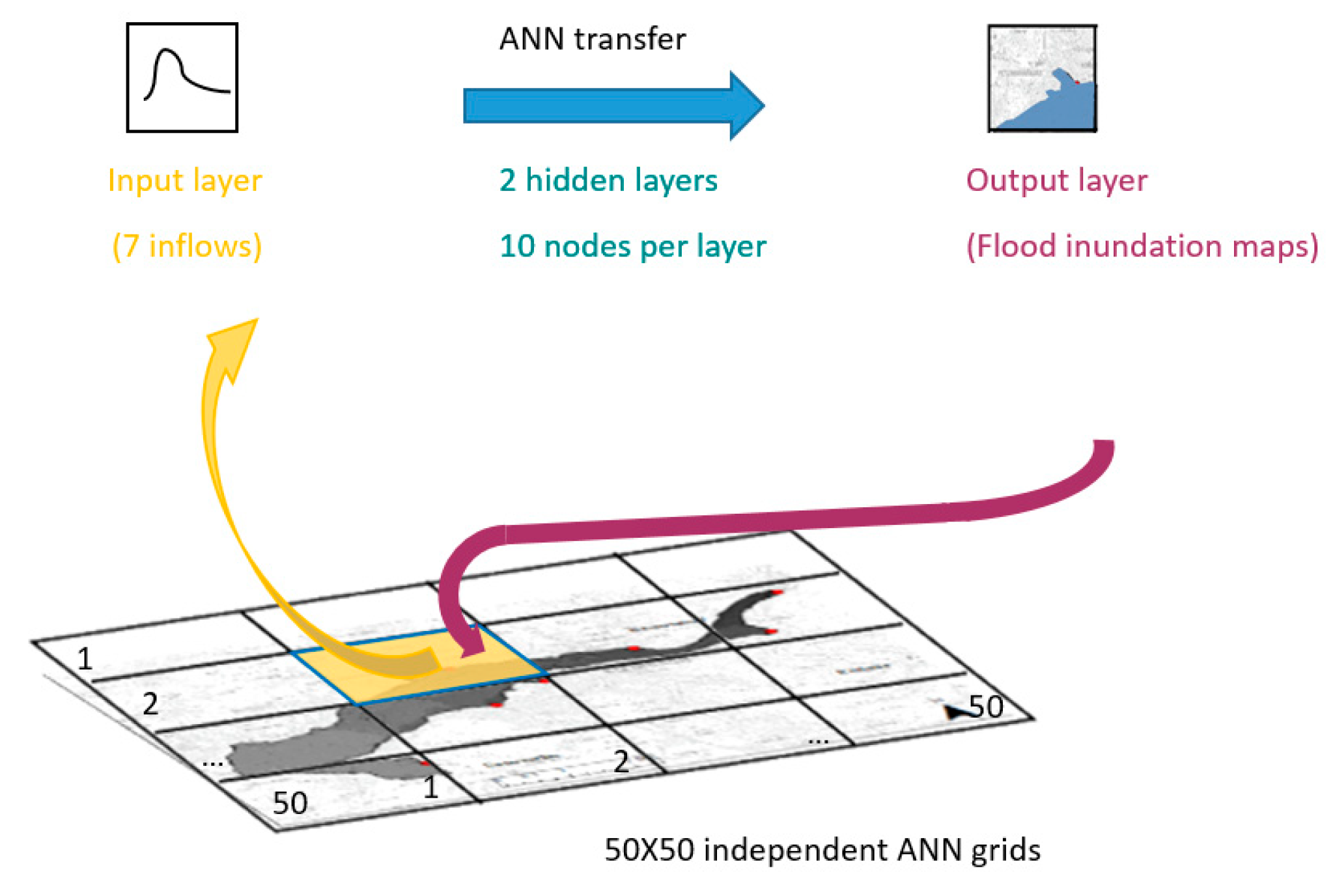
Figure 1.
The forward-feed neural network setup in the forecast study. The input layer is fed with discharge inflows of certain time interval windows. The output layer generates the flood inundation for that interval. Resilient backpropagation is applied for training this network.
Figure 1.
The forward-feed neural network setup in the forecast study. The input layer is fed with discharge inflows of certain time interval windows. The output layer generates the flood inundation for that interval. Resilient backpropagation is applied for training this network.
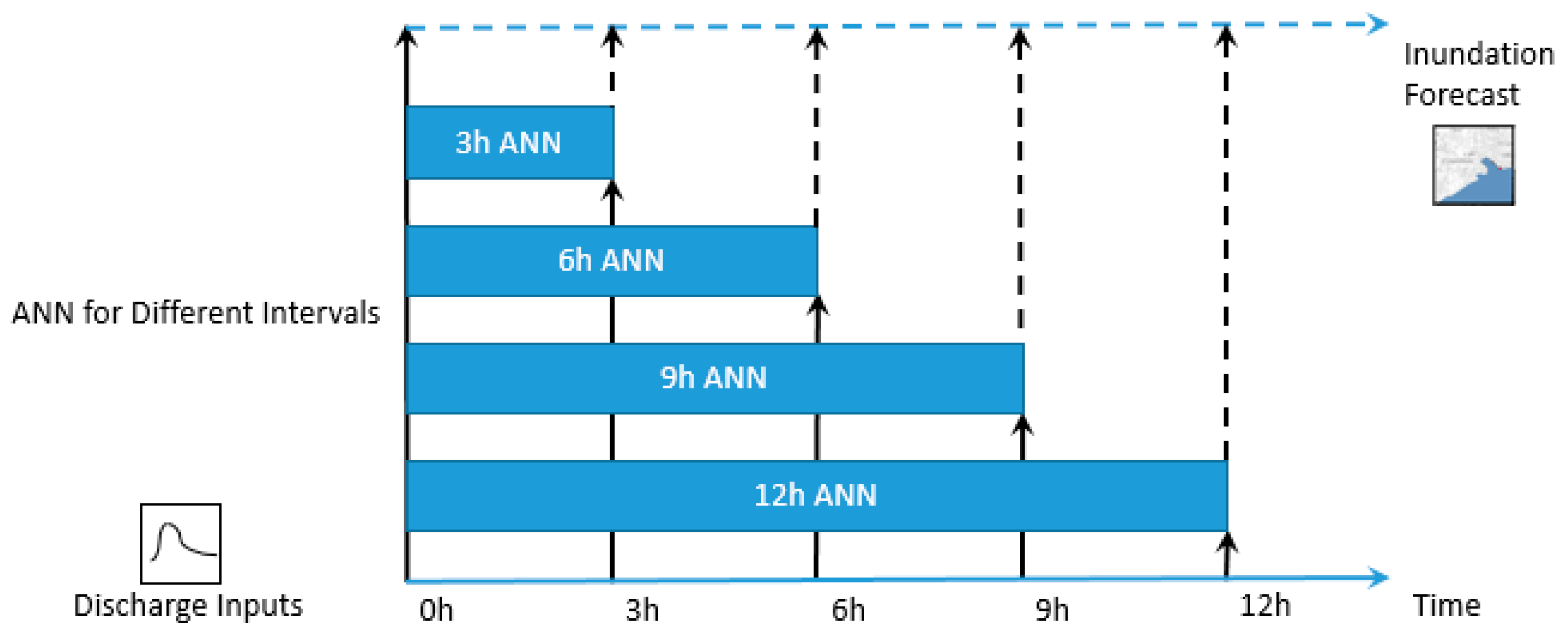
Figure 2.
Training of artificial neural networks (ANN) forecast model. Four ANN models for 3 h, 6 h, 9 h, 12 h first interval predictions are set up in this work, trained with the discharges from each synthetic flood event. After this, the models are to predict the corresponding first intervals for other events.
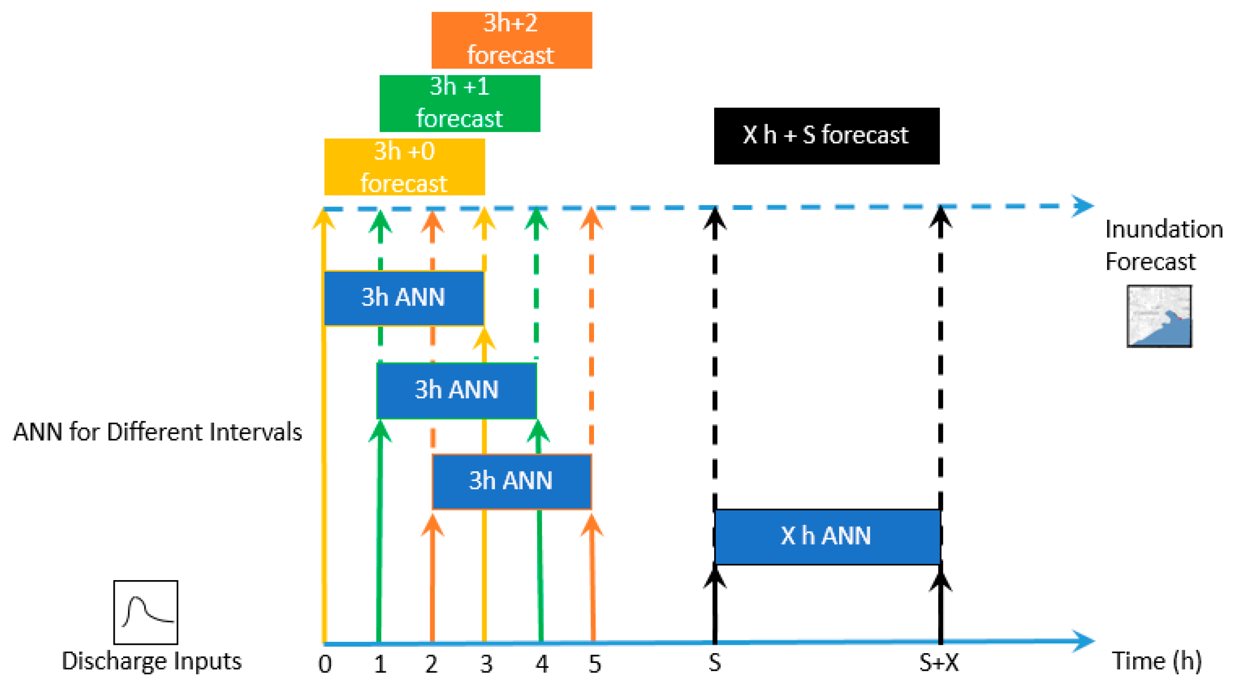
Figure 3.
Shift of ANN forecast models for multistep forecast intervals. The yellow color shows the forecast of the first interval (forecast interval same as the training interval, i.e., at time 0). The green color shows applying the original 3 h forecast network for 1 h later forecast from 1–4 h. The orange color shows applying the original 3 h forecast network for 2 h later forecast from 2–5 h. The black box shows the general case of applying the original X h forecast network for S h later forecast, from S h to X h + S.
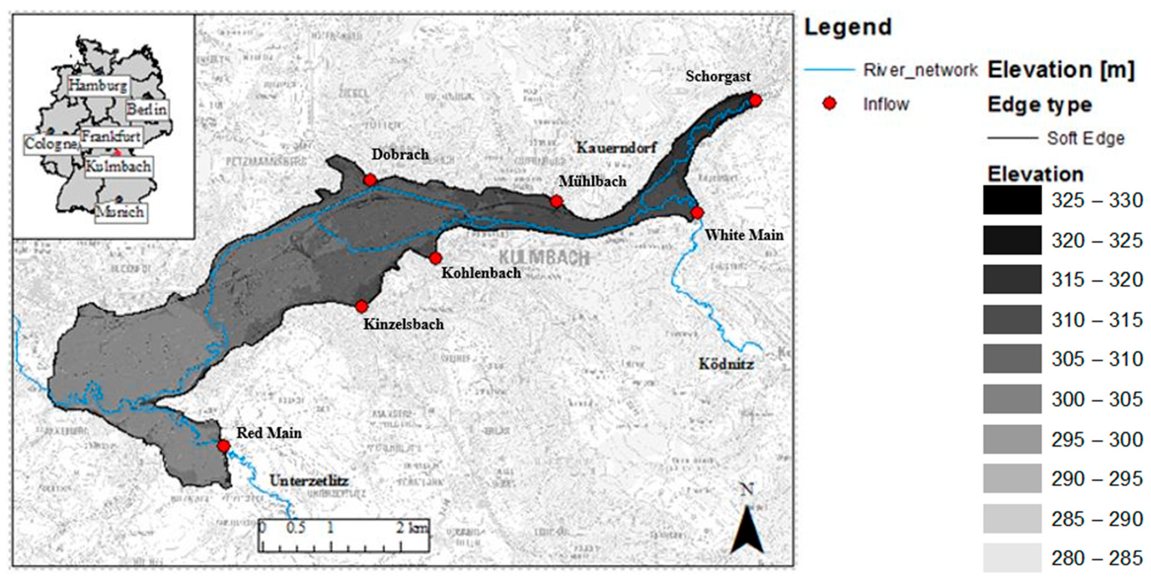
Figure 4.
Map of the study area. It shows the location of Kulmbach in Germany. The blue curves represent the river network. The shaded region is the study area with its topography represented. On the marked boundary, the red points represent the seven inflows on the boundary (three rivers and four smaller streams).
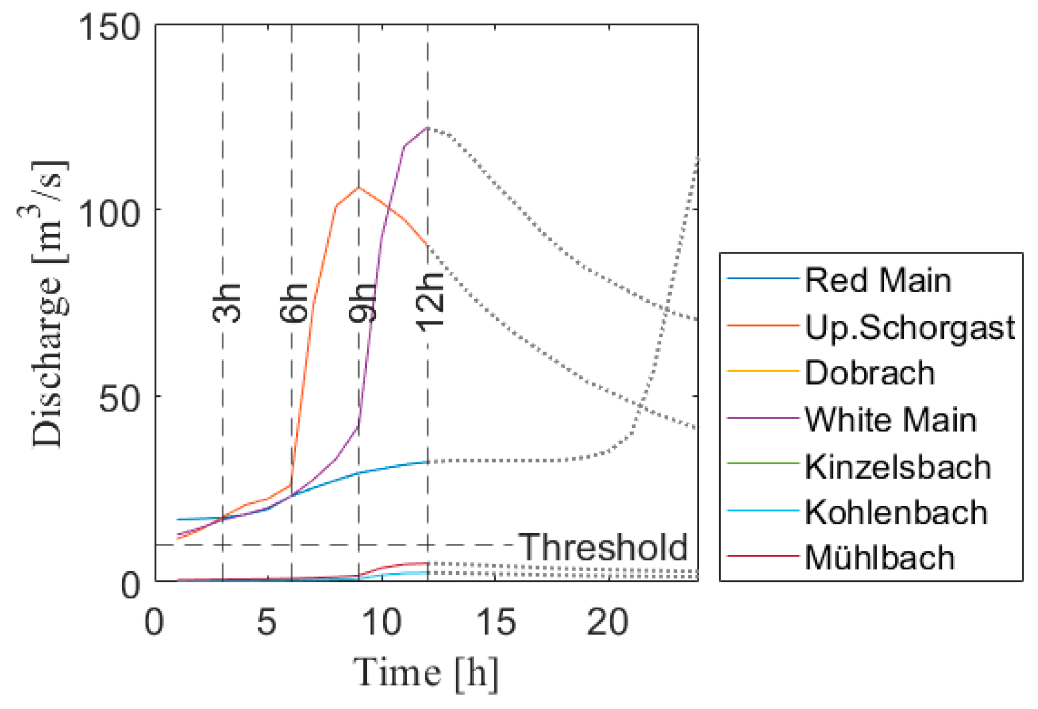
Figure 5.
Hydrographs of the flood event in 2006. Seven discharge curves of three rivers and four streams are shown in different colors. Time 0 marks the start of the prediction. The dash lines upon the discharge curves mark the different discharge sections for prediction inputs.
Figure 5.
Hydrographs of the flood event in 2006. Seven discharge curves of three rivers and four streams are shown in different colors. Time 0 marks the start of the prediction. The dash lines upon the discharge curves mark the different discharge sections for prediction inputs.
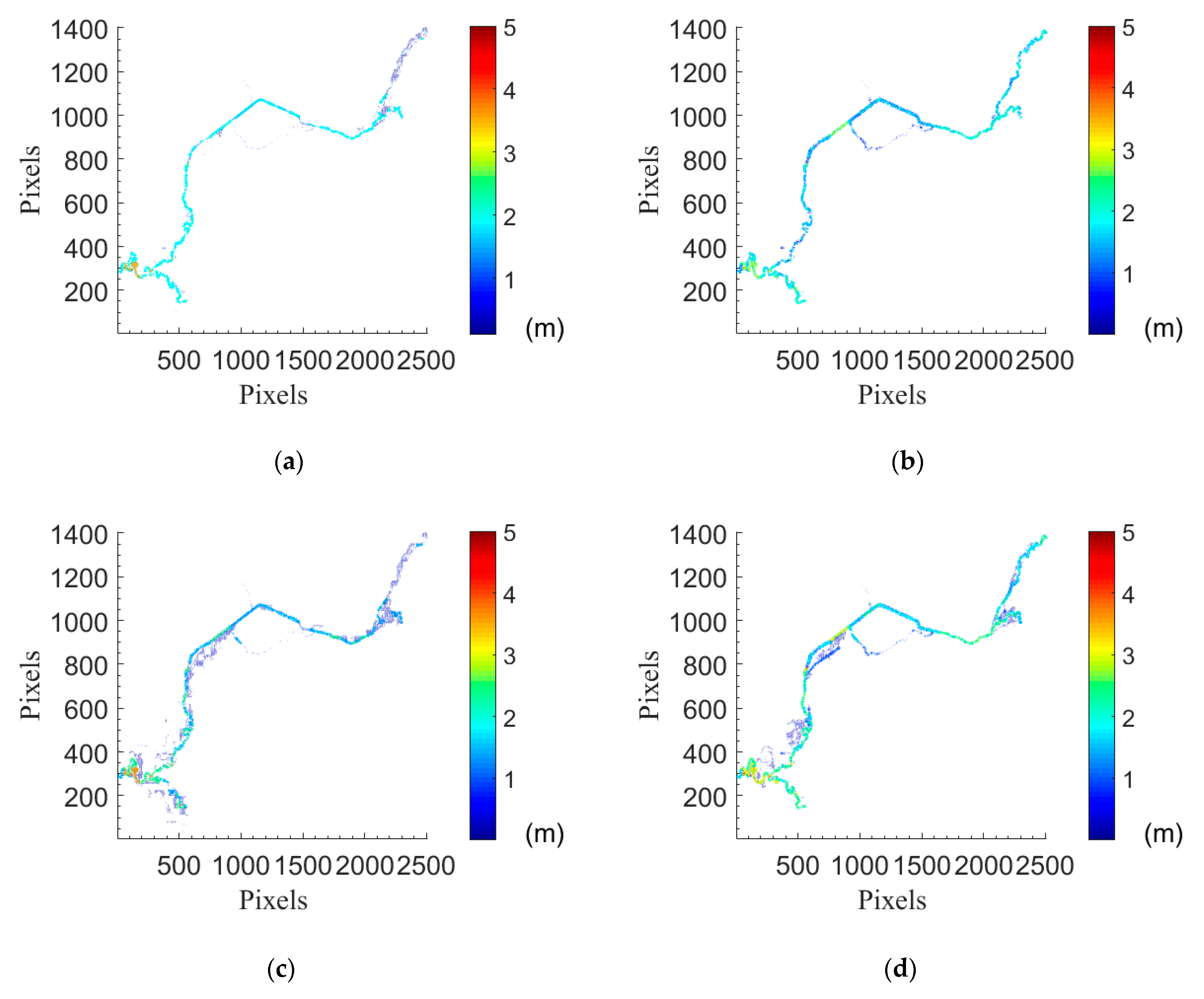
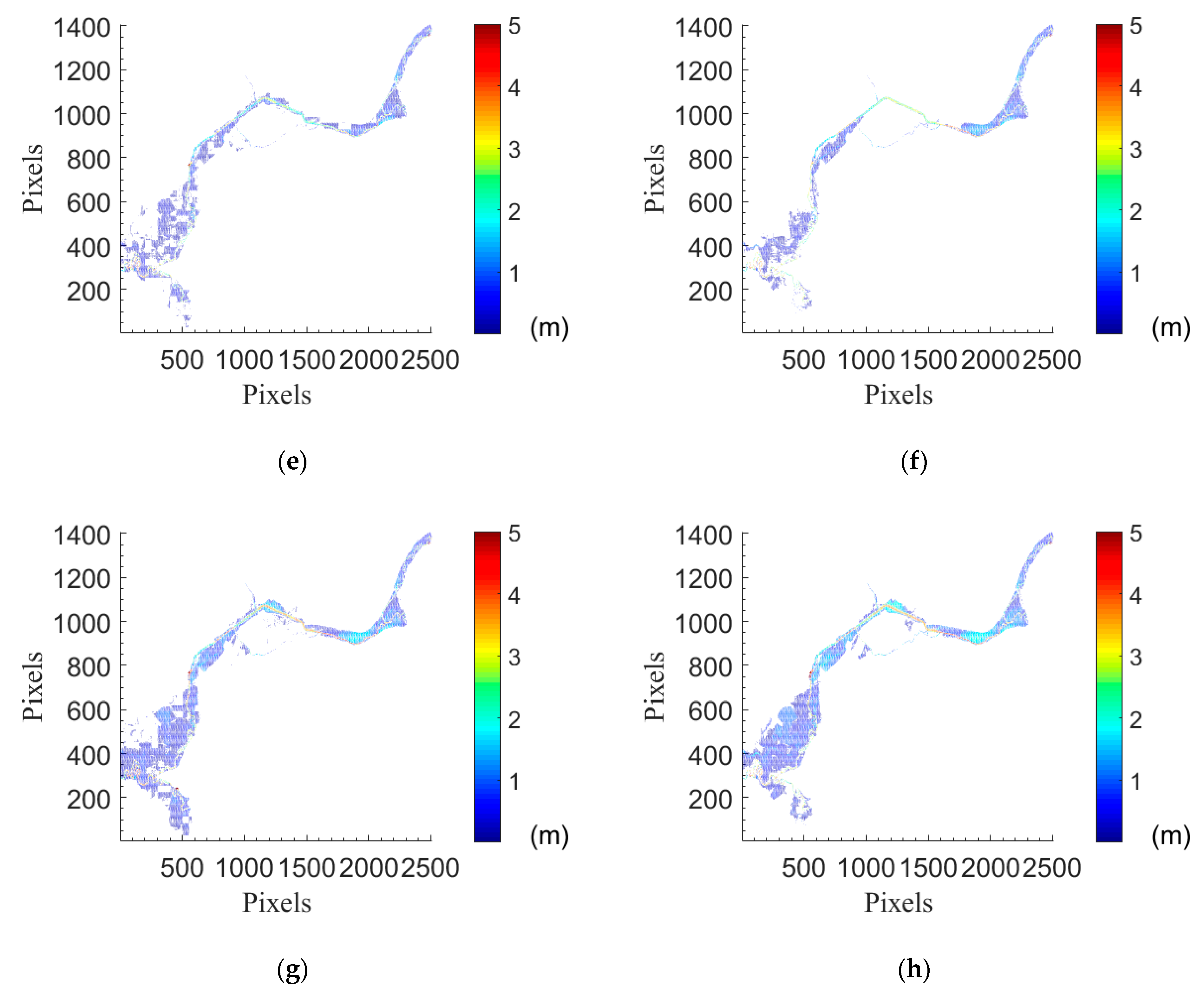
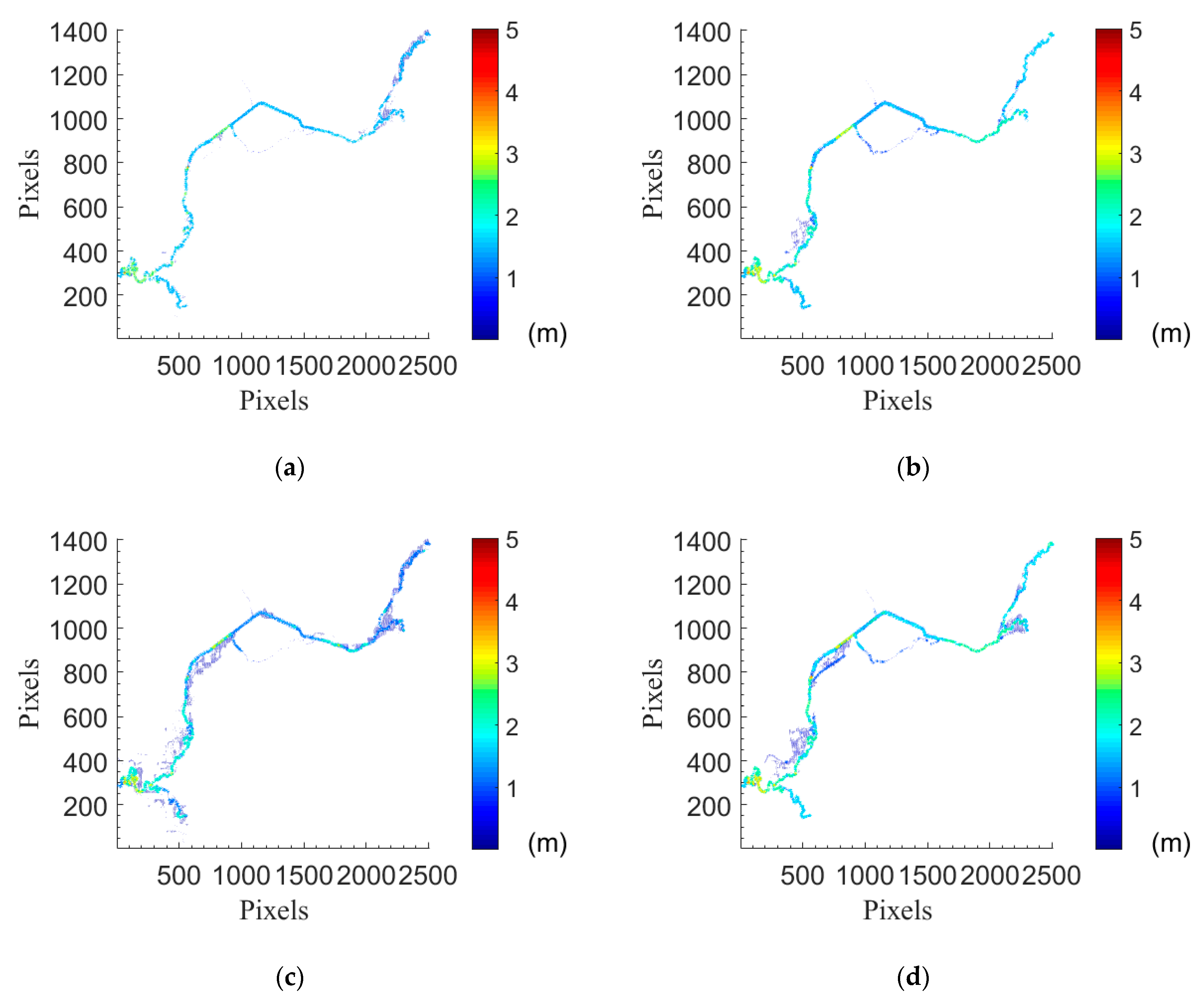
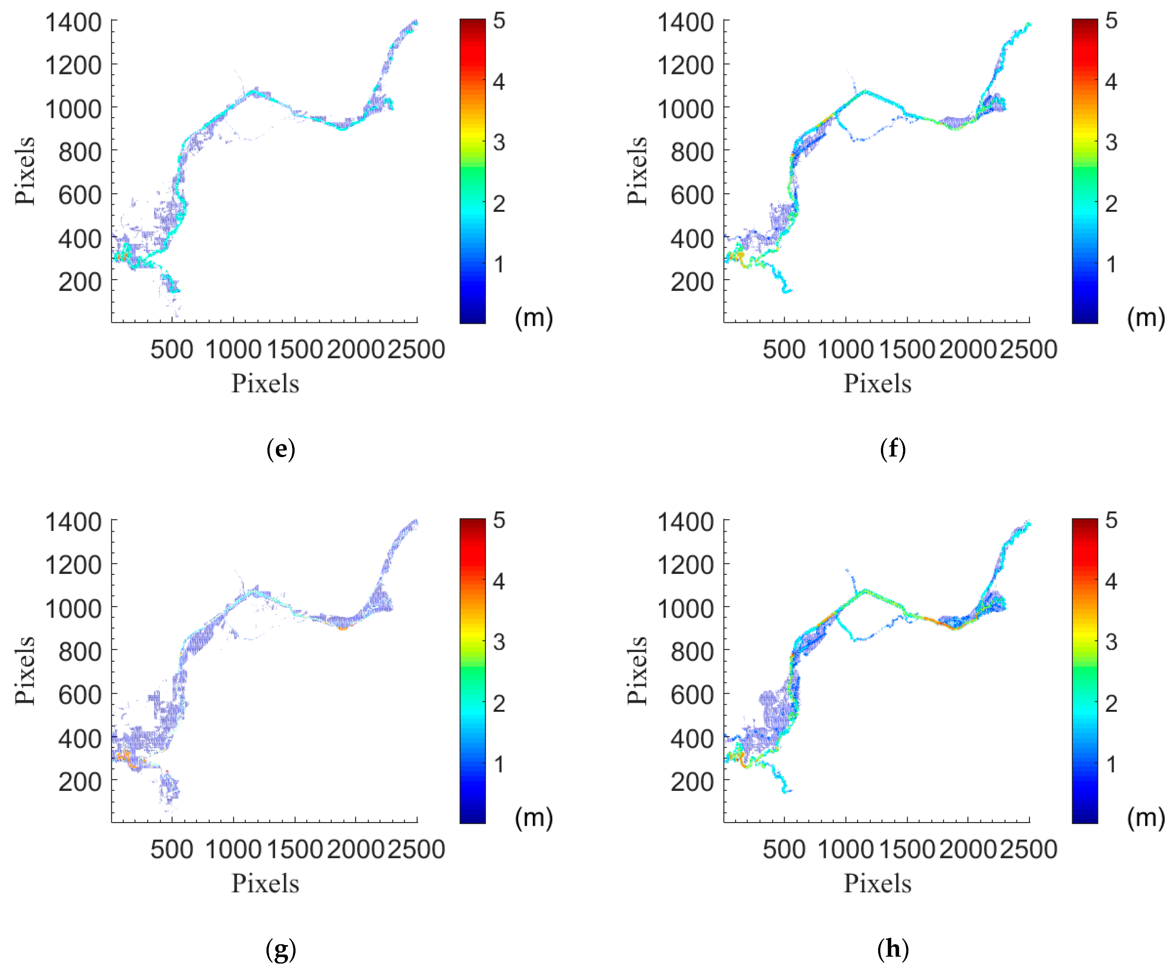
Figure 6.
Inundation maps from the prediction of water depths of the first intervals in flood event 2006. (a) ANN inundation map 3 h; (b) hydrodynamic inundation map 3 h; (c) ANN inundation map 6 h; (d) hydrodynamic inundation map 6 h; (e) ANN inundation map 9 h; (f) hydrodynamic inundation map 9 h; (g) ANN inundation map 12 h; (h) hydrodynamic inundation map 12 h.
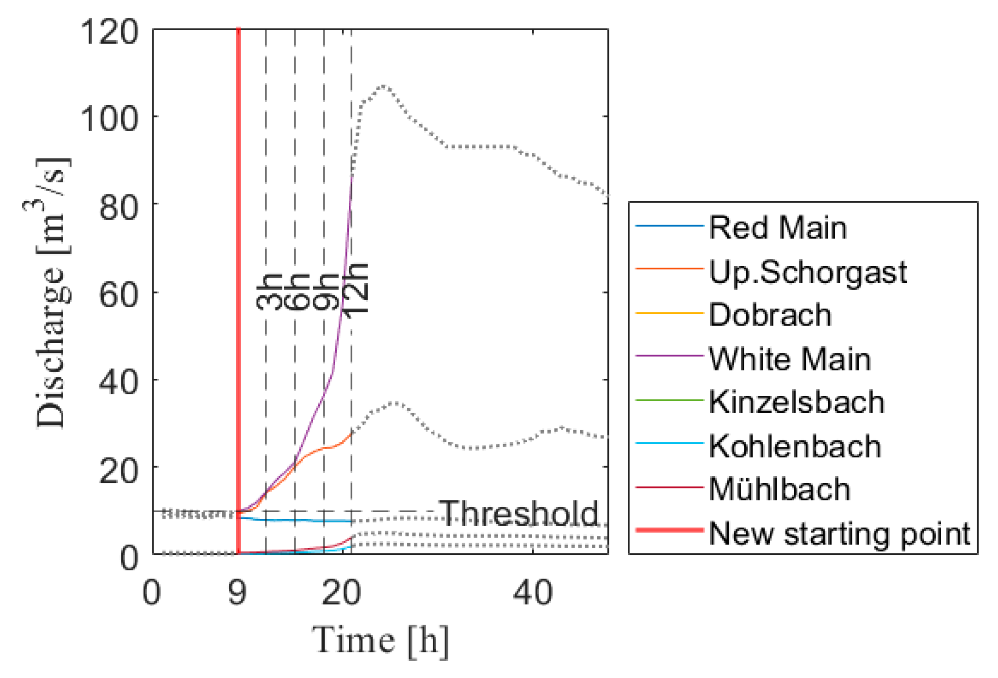
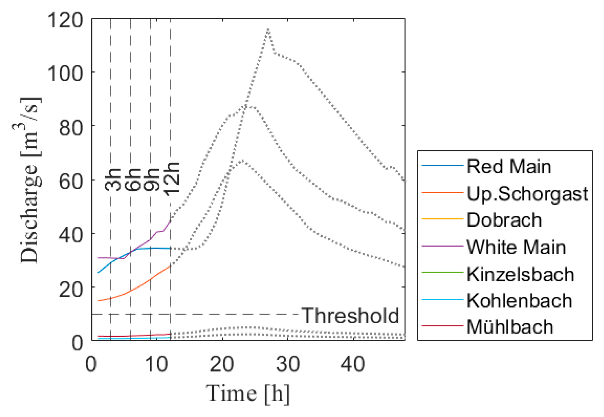
Figure 7.
Hydrographs of the flood event in 2013. Seven discharge curves of three rivers and four streams are shown in different colors. The red line time marks the new start of the prediction at 9 h, where one discharge first exceeds the forecast threshold of 10 m3/s. The dash lines upon the discharge curves mark the different discharge sections for prediction inputs.
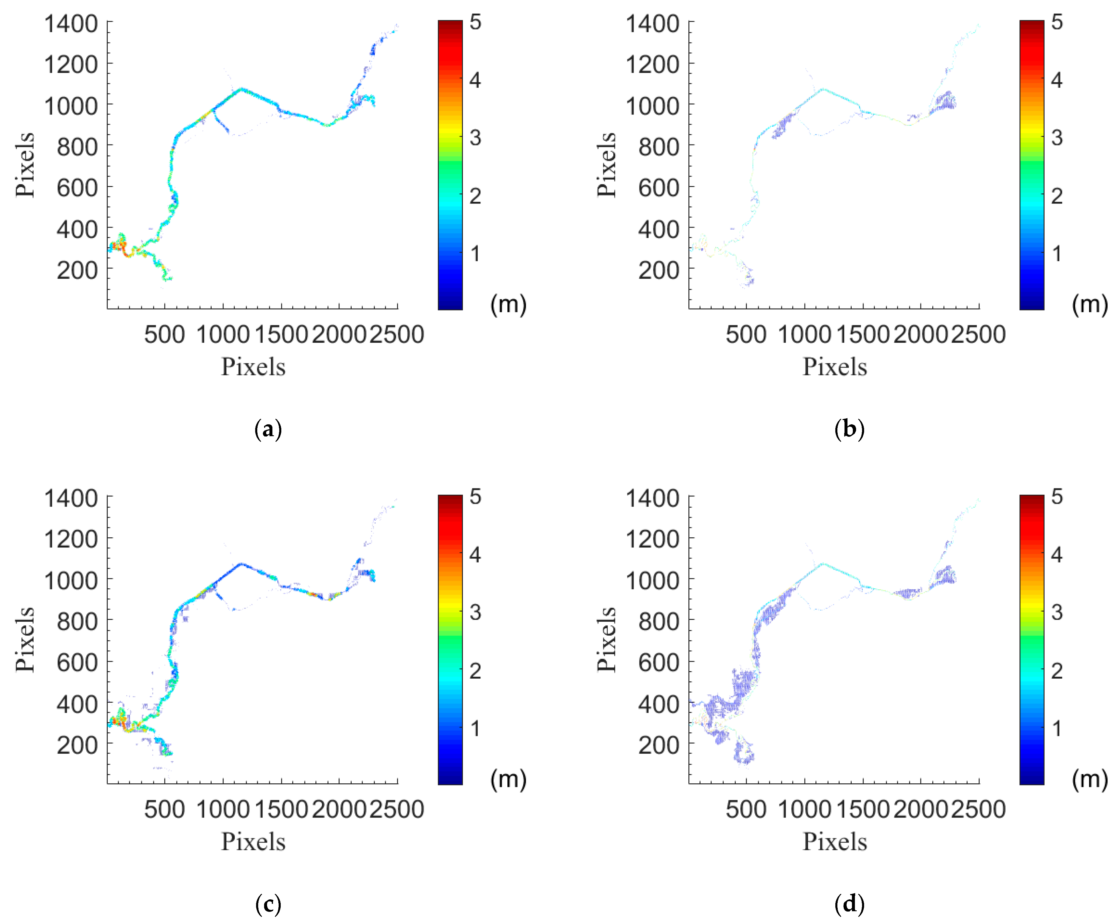
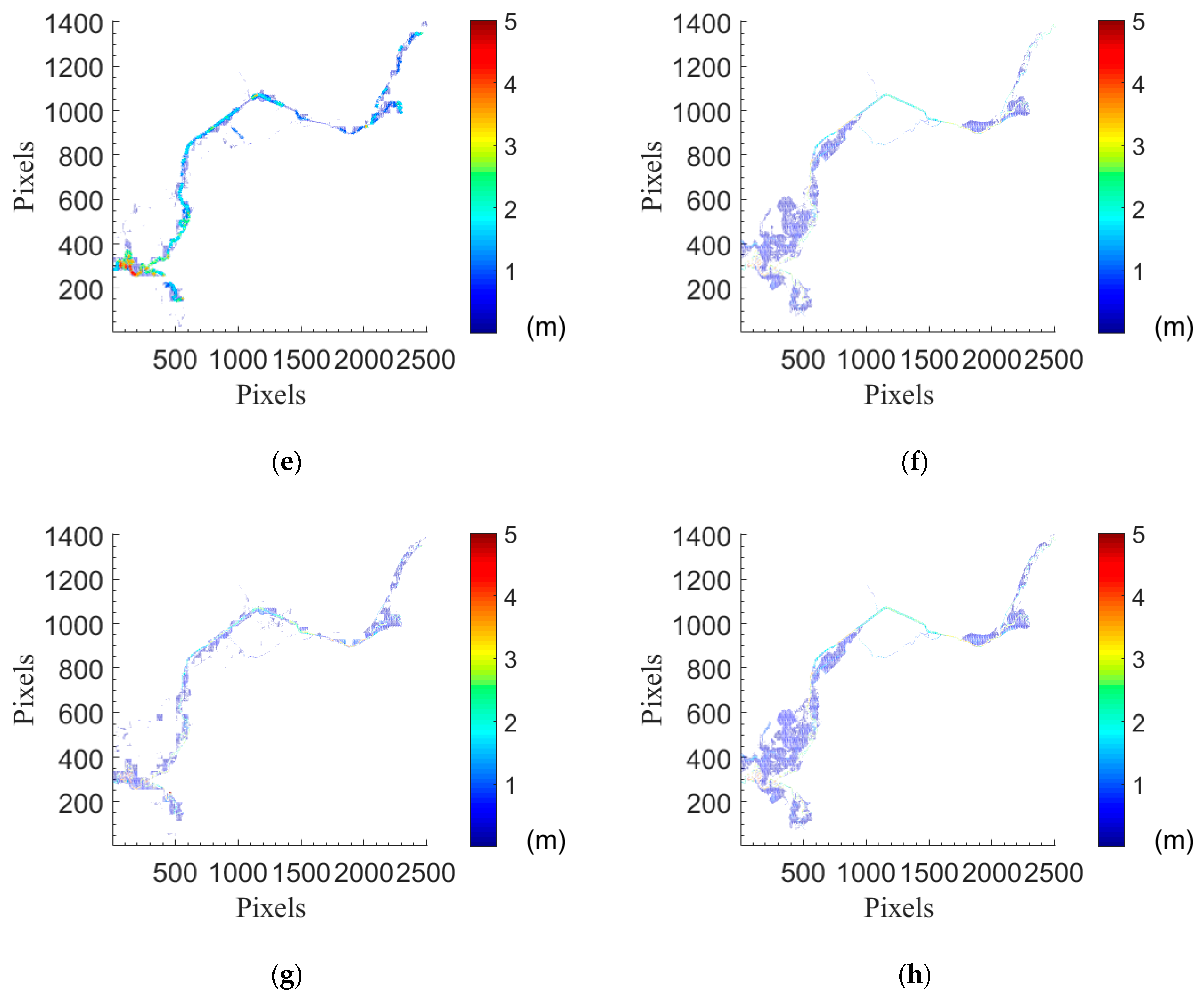
Figure 8.
Inundation maps from the prediction of water depths of the first intervals in flood event 2013. (a) ANN inundation map 3 h; (b) hydrodynamic inundation map 3 h; (c) ANN inundation map 6 h; (d) hydrodynamic inundation map 6 h; (e) ANN inundation map 9 h; (f) hydrodynamic inundation map 9 h; (g) ANN inundation map 12 h; (h) hydrodynamic inundation map 12 h.
Figure 9.
Hydrographs of the flood event in 2005. Seven discharge curves of three rivers and four streams are shown in different colors. Time 0 marks the start of the prediction. The dash lines upon the discharge curves mark the different discharge sections for prediction inputs.
Figure 9.
Hydrographs of the flood event in 2005. Seven discharge curves of three rivers and four streams are shown in different colors. Time 0 marks the start of the prediction. The dash lines upon the discharge curves mark the different discharge sections for prediction inputs.
Figure 10.
Inundation maps from the prediction of water depths of the first intervals in flood event 2005. (a) ANN inundation map 3 h; (b) hydrodynamic inundation map 3 h; (c) ANN inundation map 6 h; (d) hydrodynamic inundation map 6 h; (e) ANN inundation map 9 h; (f) hydrodynamic inundation map 9 h; (g) ANN inundation map 12 h; (h) hydrodynamic inundation map 12 h.
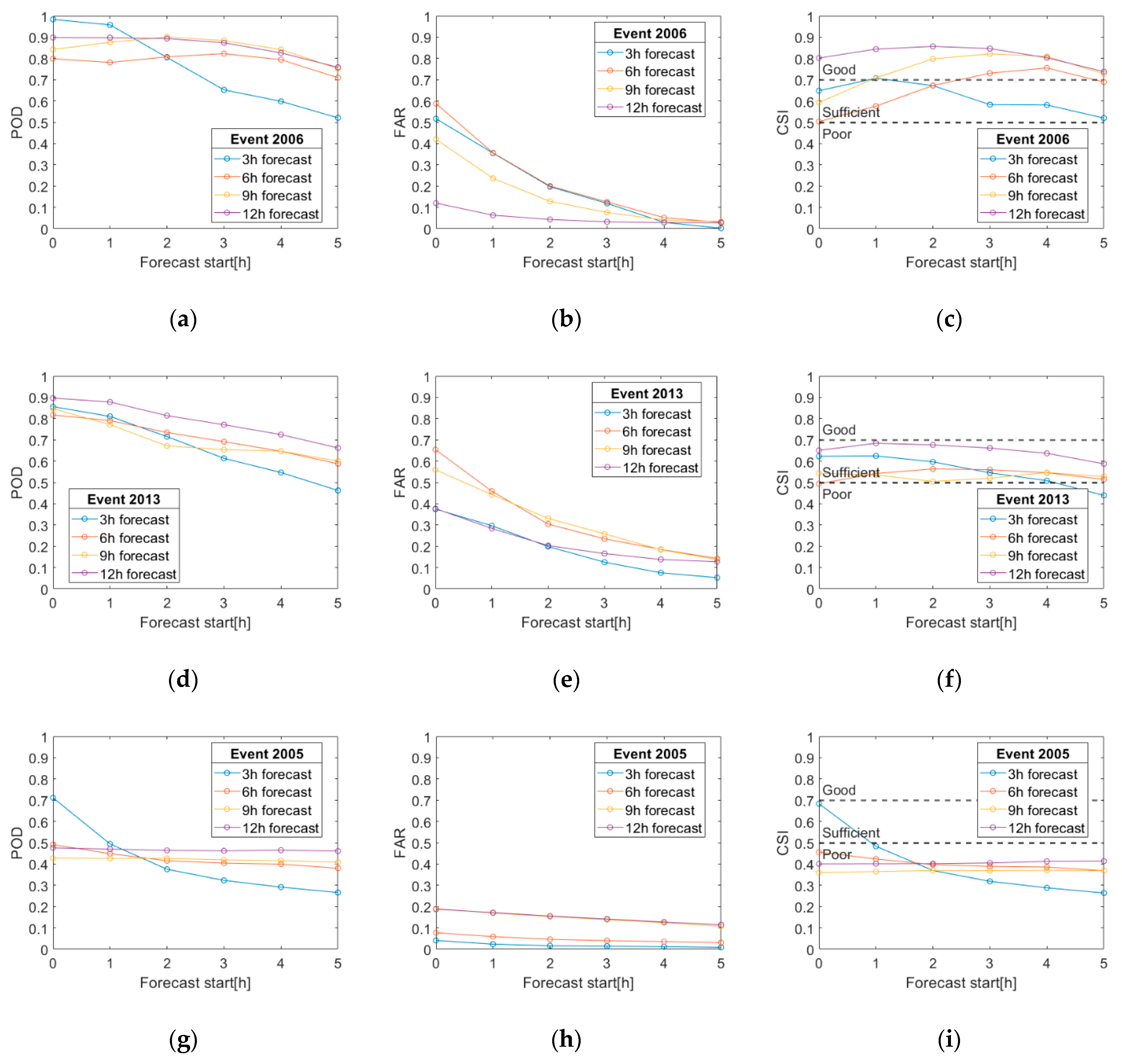
Figure 11.
Performance of the forecast of inundation extent growths by three indices. (a) probability of detection (POD) in flood event 2006; (b) false alarm ratio (FAR) in flood event 2006; (c) critical success index (CSI) in the flood event 2006; (d) POD in flood event 2013; (e) FAR in the flood event 2013; (f) CSI in flood event 2013; (g) POD in flood event 2005; (h) FAR in flood event 2005; (i) CSI in flood event 2005.
Table 1.
Number of wet grids and grid percentages of different large error thresholds for testing synthetic flood events (60 events, #121~#180).
Table 1.
Number of wet grids and grid percentages of different large error thresholds for testing synthetic flood events (60 events, #121~#180).
| Prediction Time (h) | Wet ANN Grid | ANN Grid with Average RMSE > 0.2 m | ANN
Grid% with Average RMSE ≤ 0.2 m | ANN Grid with Average RMSE > 0.3 m | ANN Grid% with Average RMSE ≤ 0.3 m | ANN Grid with Average RMSE > 0.4 m | ANN Grid% with Average RMSE ≤ 0.4 m |
|---|
| 3 | 300 | 47 | 84.33% | 18 | 94.00% | 10 | 96.67% |
| 6 | 417 | 174 | 58.27% | 78 | 81.29% | 27 | 93.53% |
| 9 | 474 | 106 | 77.64% | 37 | 92.19% | 15 | 96.84% |
| 12 | 483 | 50 | 89.65% | 12 | 97.52% | 7 | 98.55% |
Table 2.
Numbers of wet grids and accurate grid percentage for event 2006. A wet grid is with the water level over 0.1 m; any water depth below this cutoff value is eliminated. Table shows grid numbers with a larger root-mean-square error (RMSE) and their percentages to the total wet grids.
Table 2.
Numbers of wet grids and accurate grid percentage for event 2006. A wet grid is with the water level over 0.1 m; any water depth below this cutoff value is eliminated. Table shows grid numbers with a larger root-mean-square error (RMSE) and their percentages to the total wet grids.
| Prediction Time (h) | Wet ANN Grid | ANN Grid with RMSE > 0.2 m | ANN Grid% with RMSE ≤ 0.2 m | ANN Grid with RMSE > 0.3 m | ANN Grid% with RMSE ≤ 0.3 m | ANN Grid with RMSE > 0.4 m | ANN Grid% with RMSE ≤ 0.4 m |
|---|
| 3 | 280 | 46 | 83.57% | 20 | 92.86% | 6 | 97.86% |
| 6 | 405 | 84 | 79.26% | 42 | 89.63% | 25 | 93.83% |
| 9 | 474 | 134 | 71.73% | 64 | 86.50% | 36 | 92.41% |
| 12 | 483 | 157 | 67.49% | 85 | 82.40% | 47 | 90.27% |
Table 3.
Numbers of wet grids and accurate grid percentages for the flood event in 2013. A wet grid is with the water level over 0.1 m; any water depth below this cutoff value is eliminated. The table shows grid numbers with larger RMSE and their percentages to the total wet grids.
Table 3.
Numbers of wet grids and accurate grid percentages for the flood event in 2013. A wet grid is with the water level over 0.1 m; any water depth below this cutoff value is eliminated. The table shows grid numbers with larger RMSE and their percentages to the total wet grids.
| Prediction Time (h) | Wet ANN Grid | ANN Grid with RMSE > 0.2 m | ANN Grid% with RMSE ≤ 0.2 m | ANN Grid with RMSE > 0.3 m | ANN Grid% with RMSE ≤ 0.3 m | ANN Grid with RMSE > 0.4 m | ANN Grid% with RMSE ≤ 0.4 m |
|---|
| 3 | 285 | 9 | 96.84% | 2 | 99.30% | 2 | 99.30% |
| 6 | 405 | 72 | 82.22% | 27 | 93.33% | 8 | 98.02% |
| 9 | 474 | 134 | 71.73% | 65 | 86.29% | 25 | 94.73% |
| 12 | 483 | 175 | 63.77% | 104 | 78.47% | 56 | 88.41% |
Table 4.
Numbers of wet grids and accurate grid percentages for the flood event in 2005. A wet grid is with the water level over 0.1 m; any water depth below this cutoff value is eliminated. Table shows grid numbers with larger RMSE and their percentages to the total wet grids.
Table 4.
Numbers of wet grids and accurate grid percentages for the flood event in 2005. A wet grid is with the water level over 0.1 m; any water depth below this cutoff value is eliminated. Table shows grid numbers with larger RMSE and their percentages to the total wet grids.
| Prediction Time (h) | Wet ANN Grid | ANN Grid with RMSE > 0.2 m | ANN Grid% with RMSE ≤ 0.2 m | ANN Grid with RMSE > 0.3 m | ANN Grid% with RMSE ≤ 0.3 m | ANN Grid with RMSE > 0.4 m | ANN Grid% with RMSE ≤ 0.4 m |
|---|
| 3 | 280 | 65 | 76.79% | 36 | 87.14% | 19 | 93.21% |
| 6 | 405 | 165 | 59.26% | 115 | 71.60% | 74 | 81.73% |
| 9 | 474 | 216 | 54.43% | 148 | 68.78% | 93 | 80.38% |
| 12 | 483 | 244 | 49.48% | 168 | 65.22% | 107 | 77.85% |
Table 5.
Forecast accuracy percentages for the flood event in 2006. This table shows the grid percentage to the total wet grids with average RMSE within 0.3 m. The forecast begins by the starting point, several hours later than the event beginning for the real-time forecast.
Table 5.
Forecast accuracy percentages for the flood event in 2006. This table shows the grid percentage to the total wet grids with average RMSE within 0.3 m. The forecast begins by the starting point, several hours later than the event beginning for the real-time forecast.
| Starting Point (h) | Prediction Interval (h) |
|---|
| 3 | 6 | 9 | 12 |
|---|
| +1 | 98.93% | 92.10% | 83.12% | 79.09% |
| +2 | 98.94% | 90.86% | 77.85% | 79.92% |
| +3 | 96.94% | 89.38% | 76.58% | 78.26% |
| +4 | 95.11% | 86.95% | 70.89% | 75.36% |
| +5 | 86.60% | 69.29% | 66.88% | 68.12% |
Table 6.
Forecast accuracy percentages rate for the flood event in 2013. This table shows the grid percentage to the total wet grids with average RMSE within 0.3 m. The forecast begins by the starting point, several hours later than the event beginning for the real-time forecast.
Table 6.
Forecast accuracy percentages rate for the flood event in 2013. This table shows the grid percentage to the total wet grids with average RMSE within 0.3 m. The forecast begins by the starting point, several hours later than the event beginning for the real-time forecast.
| Starting Point (h) | Prediction Interval (h) |
|---|
| 3 | 6 | 9 | 12 |
|---|
| +1 | 99.30% | 92.59% | 84.18% | 72.67% |
| +2 | 98.95% | 89.88% | 78.90% | 70.39% |
| +3 | 96.30% | 89.17% | 75.74% | 67.91% |
| +4 | 94.17% | 82.51% | 68.78% | 67.29% |
| +5 | 91.28% | 77.34% | 66.46% | 66.67% |
Table 7.
Forecast accuracy percentages for the flood event in 2005. This table shows the grid percentages to the total wet grids with average RMSE within 0.3 m. The forecast begins by the starting point, several hours later than the event beginning for the real-time forecast.
Table 7.
Forecast accuracy percentages for the flood event in 2005. This table shows the grid percentages to the total wet grids with average RMSE within 0.3 m. The forecast begins by the starting point, several hours later than the event beginning for the real-time forecast.
| Starting Point (h) | Prediction Interval (h) |
|---|
| 3 | 6 | 9 | 12 |
|---|
| +1 | 83.74% | 69.95% | 66.89% | 63.15% |
| +2 | 81.67% | 68.23% | 64.77% | 61.70% |
| +3 | 76.31% | 67.00% | 63.08% | 60.25% |
| +4 | 74.85% | 66.50% | 60.97% | 60.25% |
| +5 | 70.97% | 61.08% | 58.65% | 60.25% |


