The Influence of Freshwater Discharge and Wind Forcing on the Dispersal of River Plumes Using a Three-Dimensional Circulation Model

Abstract

Tidal estuaries provide crucial pathways for contaminant transport. The salinity levels in estuaries and coasts are conserved substances that function as natural tracers to easily understand the offshore transport of substances that are subject to environmental factors. A three-dimensional (3D) circulation and mass transport model were utilized to delineate the salinity plume in a tidal estuary and continental shelf. The numerical modeling results were compared with the tidal amplitudes and phases, velocities, and salinities at different gauging stations in 2017. Quantitatively, the simulation and measurement results are in reasonably good agreement. Furthermore, the validated model was adopted to estimate the recovery times in tidal estuaries that are subjected to extreme freshwater discharges that come from the upstream reaches during typhoon events and to analyze the influences of freshwater discharge and wind stress on the river plume around the continental shelf. The simulated results revealed that the salinity recovery time at the river mouth due to Typhoon Saola in 2012 was less than 8 days. Increased inputs from freshwater discharge resulted in changes in the distances and areas of the river plumes. Linear regression relationships between the plume distance/plume area and the total freshwater discharge inputs were established. Neap and high slack tides were associated with the maximum plume distances and areas. Excluding tidal forcing resulted in larger plume distances and areas compared to the case in which tidal forcing was considered. The southward-favorable and northward-favorable plumes were controlled by northeasterly winds and southwesterly winds, respectively. The relative importance of freshwater discharges and wind forcing was explored. The results indicate that freshwater discharges frequently dominated the river plume, except when strong southwesterly or northeasterly winds prevailed.

1. Introduction

Estuaries provide important pathways for the transport of sediments, nutrients, and pollution to coastal oceans. Therefore, understanding the coupled interactions between estuaries and their adjacent coastal oceans is crucial to better understand the fate and transport of river-borne terrigenous contaminants that flow to continental shelf environments [1,2,3,4,5,6,7]. The river discharge-induced fresh-to-salt water stratification with buoyancy significantly affects the hydrodynamics in tidal estuaries and transports the biochemistry from estuaries to shelf environments to form a surface river plume [8,9,10,11]. The freshening water nearshore as a result of river discharge is one of the mechanisms that dominate the stratification and circulation in coastal areas Kourafalou [12] and Garvine [13] defined river plumes as plumes of buoyant water that are produced by inflow from a buoyancy source. The transport and fate of plumes along the pathway onto the continental shelf depend on environmental factors, including river discharges and wind stresses.

Many external driving forces, including river discharges, Coriolis forces, tides, winds, and tidal currents, have critical influences on the dispersal of river plumes [10,14,15,16,17]. Although there are many external forcings that affect river plumes, different approaches have been adopted to explore the dynamics of surface river plumes in estuaries, including remote sensing [18,19,20], field observations [21,22,23], theoretical analyses [24,25,26,27], and numerical investigations [28,29,30,31,32,33,34,35,36]. Among these approaches, numerical modeling [37] is a popular and widely used method to explore the influence of different environmental factors on surface river plumes in coastal seas and continental shelves. In terms of the modeling frameworks, one-dimensional (1D) models widely applied in river studies are unable to describe the horizontal variations in coastal seas. Horizontal two-dimensional (2D) models consider spatial variations but do not resolve the vertical stratification that is present in estuaries and coastal seas. Therefore, 3D models are particularly suitable for resolving the spatial and vertical variations. In addition, the river plume dispersal in offshore waters can be explored using salinity concentration since salt is a conservative substance without any chemical reaction with others.

The objective of this study was to examine the effects of freshwater discharges, tides, and winds on the river plumes in the Danshuei River estuarine system. In particular, the Danshuei River estuarine system was subject to serious pollutants resulting from point sources and nonpoint sources [38]. Thus, understanding the pollutant plumes on the continental shelf is a crucial issue for environmental management. The SCHISM-based three-dimensional circulation model for the study area was developed. To ascertain the model capability and availability, the modeling results of tidal amplitudes and phases, currents, and salinities were compared with the measured data collected in 2017 at different gauging stations in the Danshuei River estuary. After validation, the model was further employed to estimate the recovery times and to explore the influences of freshwater discharges, tidal actions, and wind forcings on salinity plumes on the continental shelf.

This article is organized as follows. Section 2 describes the study area, and Section 3 illustrates the methods, including the model description, model configuration and setup, and the statistical errors in the model performance. The model-to-data comparisons among the hydrodynamics, salinities, and the influences of different environmental factors on the dispersal of river plumes are presented in Section 4. A discussion of river discharges and wind stresses is introduced in Section 5. Finally, the conclusions are summarized in Section 6.

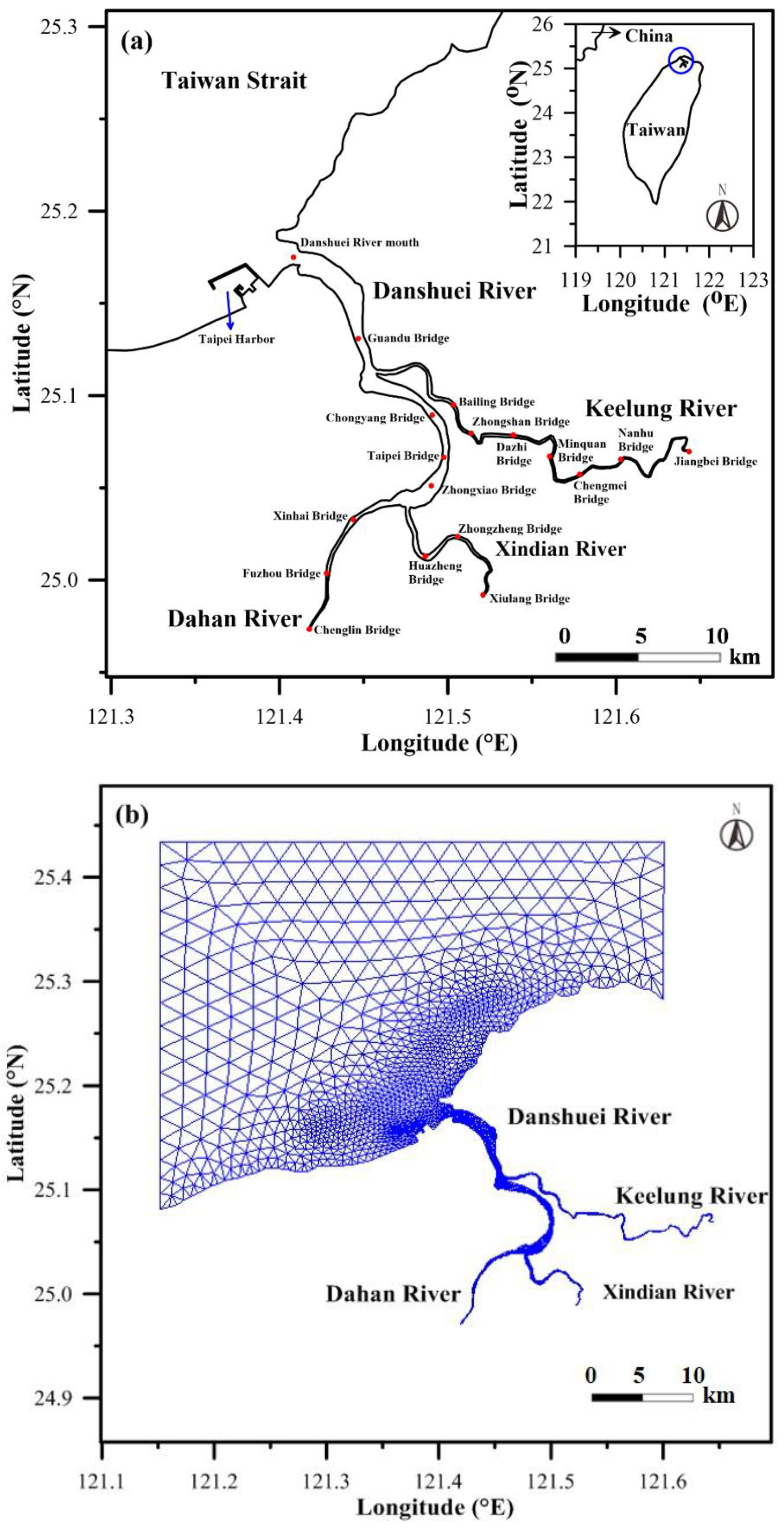
2. Description of the Study Area

Three major tributaries, the Dahan River, Xindian River, and Keelung River, comprise the estuarine system, which covers a total watershed area of 2728 km² (Figure 1a). Based on the measurement records from 1990 to 2017 (provided by the Water Resources Agency), the peak discharges for a 200-year return period are 13,200 m³/s, 11,600 m³/s, and 5350 m³/s in the Dahan, Xindian, and Keelung Rivers [39], while their average freshwater discharges are 29.18 m³/s, 60.84 m³/s, and 26.68 m³/s, respectively. The freshwater discharges at different exceedance probabilities for the upriver sections of these three tributaries are shown in

Table 1. Freshwater discharge inputs at the upstream reaches of three major tributaries.

Discharge with Exceedance Probability	Dahan River (m3/s)	Xindian River (m3/s)	Keelung River (m3/s)	Total Freshwater Discharge (m3/s)
Q10	64.78	131.36	67.00	263.14
Q20	31.79	79.40	35.66	146.85
Q30	19.33	53.80	21.50	94.63
Q40	12.55	38.37	14.00	64.92
Q50	8.52	27.10	9.53	45.15
Q60	5.98	20.08	6.46	32.52
Q70	4.32	14.22	4.38	22.92
Q80	3.19	9.01	2.72	14.92
Q90	2.19	3.76	1.33	7.28

. For example, a Q₉₀ flow stands for a very low flow but with an occurrence probability of 10%. The table indicates that the Q₉₀ flows in the upstream reaches of the three tributaries are 2.19 m³/s, 3.75 m³/s, and 1.33 m³/s, respectively. The principal tidal constituent is the principal lunar semidiurnal tide (e.g., M₂ tide). The water level and tidal current variations are dominated by tidal propagation from the coastal sea to the estuary. The mean tidal range, neap tidal range, and spring tidal range in the tidal estuary are 2.22 m, 0.85 m, and 3.1 m, respectively [40]. The tidal limits of the astronomical tides reach the Chenlin Bridge in the Dahan River, Xiulang Bridge in the Xindian River, and Jiangbei Bridge in the Keelung River (Figure 1a) [41].

The net upriver flows in the bottom layer are induced by saltwater intrusion, and the net downriver flows in the upper layer result from freshwater discharge due to two-layer circulation. The salinity variations change with the ebb and flood tidal flows and respond to freshwater discharge inputs [42]. The limit of salt intrusion reaches Xinhai Bridge in the Dahan River during low flow conditions [41]. According to the long-term wind records obtained from the Taiwan Central Weather Bureau (CWB), two prevailing wind directions occur in Taiwan. During the spring and summer seasons, southwesterly winds frequently occur, while during the autumn and winter seasons, northeasterly winds prevail. According to data gathered from the CWB, wind speeds ranging from 6 to 20 m/s are associated with moderate to strong winds.

3. Methods

3.1. Model Description

A semi-implicit cross-scale hydroscience integrated system model called SCHISM [43,44] that utilizes mixed triangular –quadrangular unstructured grids in the horizontal dimension and Localized Sigma Coordinates with Shaved Cells (LSC²) in the vertical direction was employed in the present study. The SCHISM was originally developed and derived from the semi-implicit Eulerian–Lagrangian finite element model (SELFE) [45]. The model solves the Navier–Stokes equations, including the continuity, momentum, and salt transport equations, with hydrostatic approximations. The SCHISM uses semi-implicit finite element and finite volume methods with an Eulerian–Lagrangian approach to solve the governing equations. Because mixing high-order with low-order approaches is used for the numerical algorithms, stable and accurate results can be obtained. The generic length-scale model with a stability function for turbulence closure schemes (k-kl, k-ω, and k-$\epsilon$) [46,47] was built in the SCHISM. Ye et al. [48] tested these three turbulence closure schemes and found that the results were similar. Therefore, the k-kl turbulence closure model was adopted in this study. Note that the eddy viscosities and diffusivities respectively for the momentum and tracers are related to turbulent kinetic energy, turbulence mixing length, and stability functions. The ratio between the eddy diffusivity and turbulent diffusivity was determined using a constant Schmidt number, that is, 1.96 [47]. The background diffusivity was set to 10⁻⁶ m²/s. A constant drag coefficient of 2.5 × 10⁻³ was used at the bottom boundary layer. The minimum depth was set to 0.01 m and was used for the wetting and drying simulations.

The salt transport equation can be expressed as follows:

$$\frac{\partial s}{\partial t}+\frac{\partial (us)}{\partial x}+\frac{\partial (vs)}{\partial y}+\frac{\partial (ws)}{\partial z}=\frac{\partial }{\partial x}(K_x\frac{\partial s}{\partial x})+\frac{\partial }{\partial y}(K_y\frac{\partial s}{\partial y})+\frac{\partial }{\partial z}(K_z\frac{\partial s}{\partial z})$$

(1)

where $s$ is the salinity; u, v, and w denote the velocity component in the x, y, and z directions, respectively; t is the time; K_x, K_y, and K_z express the turbulent diffusivities in the x, y, and z directions, respectively. The velocity fields obtained from solving the continuity and momentum equations were substituted into the salt transport Equation (1) to yield the salinity.

A detailed explanation of the numerical solution methods, turbulence closure model, and numerical stability can be found in the work by Zhang et al. [43,44].

3.2. Model Setup for Simulation

The measured geomorphology data for the studied continental shelf and estuarine system were obtained from Taiwan’s Ocean Data Bank and the Water Resources Agency, respectively, and were utilized to produce meshes/grids in the horizontal dimension for the model simulations (Figure 1b). The meshes for the Danshuei River estuarine system and continental shelf consist of 20,448 elements/11,433 nodes. Different grid resolutions were adopted for the continental shelf and estuarine system to decrease the computational times. A fine-grid resolution was adopted for the estuarine system, containing grid sizes of 40 m, 42 m, and 35 m in the upper reaches of the Dahan, Xindian, and Keelung Rivers, respectively. The grid size at the river mouth of the Danshuei River was approximately 170 m. A coarse-grid resolution was used at the open boundaries, with a grid size of 2400 m. The vertical dimension consisted of 10 evenly spaced sigma layers. A 120-s computational time step was adopted for the model runs to guarantee numerical stability.

The open boundary conditions at the coastal sea were specified by the water elevations and salinities. The water elevation time series that was produced from five tidal constituents (e.g., M₂, S₂, N₂, K₁, and O₁) at the open sea boundaries, which were calculated from tidal driver software [49], was utilized to drive the model simulations. Due to the absence of measured salinity data, the salinities at the open boundaries were set to 35 ppt. Note that the water temperature was not simulated in the present study. Considering that tidal waves can affect water elevations and flow variations, the freshwater discharges at the upstream boundaries were defined at locations far from the coastal sea. This means that the upstream boundary conditions located at the upper reaches of the tide limit were specified by using freshwater discharges.

For the model-data comparison (i.e., validation), the simulation period was from April to September 2017, with the atmospheric forcing from observations (real wind speed and direction). Further, to investigate the effects of freshwater discharge, tidal forcing, and wind forcing on salinity plumes on the continental shelf, a number of scenario simulations were designed (see

Table 2. Model configurations for scenario simulations.

Scenario Simulation	Freshwater Discharge	Tide	Wind
Effect of freshwater discharge	Peak flows were taken from Typhoon Saola event combined with normal flow at upstream boundaries	Water surface elevations at open boundaries were generated using five tidal components	off
Effect of tidal forcing	Mean discharges at upstream boundaries	Water surface elevations at open boundaries were generated using five tidal components and without tidal effect	off
Effect of wind forcing	Mean discharges at upstream boundaries	Water surface elevations at open boundaries were generated using five tidal components	Speeds: 6 and 20 m/s Directions: northeasterly, southwesterly, northwesterly, and southeasterly

for model configurations).

3.3. Model Performance Evaluation

Various statistical error indices can be found in the literature [50] to evaluate the model prediction capabilities. However, no standard procedure is used for model validations. In the present study, five indices were adopted to compare the model simulation results and measurement data to evaluate the performance of the circulation model. These indices for model performance include the root mean square error (RMSE), mean absolute percentage error (MAPE), correlation coefficient (CC), skill score (SS, [51]), and Nash–Sutcliffe model efficiency index (NSE, [52]). These indices can be expressed by Equations (2)–(5), as follows:

$$MAPE=\frac{1}{N}{\displaystyle \sum _{i=1}^N\left|\frac{P_i-M_i}{M_i}\right|}\times 100\%$$

(2)

$$CC=\frac{{\displaystyle \sum _{i=1}^N(P_i-\stackrel{\_}{P})(M_i-\stackrel{\_}{M})}}{\sqrt{{\displaystyle \sum _{i=1}^N{(P_i-\stackrel{\_}{P})}^2}}\sqrt{{\displaystyle \sum _{i=1}^N{(M_i-\stackrel{\_}{M})}^2}}}$$

(3)

$$SS=1-\frac{{\displaystyle \sum _{i=1}^N{\left|P_i-M_i\right|}^2}}{{\displaystyle \sum _{i=1}^N{(|P_i-\stackrel{-}{M}|+|M_i-\stackrel{\_}{M}|)}^2}}$$

(4)

$$NSE=1-\frac{{\displaystyle \sum _{i=1}^N{(P_i-M_i)}^2}}{{\displaystyle \sum _{i=1}^N{(M_i-\overline{M})}^2}}$$

(5)

where N defines the total number of data points; P_i and M_i express the values of the ith data of the predictions and measurements in the time series, respectively; $\overline{M}$ denotes the mean value of the measurements. Smaller RMSE and MAPE values indicate better model performance. The CC values denote the strength and direction between the predicted and measured data and fall in the range from −1 to 1. The value of CC equals 1, which represents the linear equation that defines a perfect relationship between the predicted and measured data. A value of 1 indicates perfect performance of the circulation model, values ranging from 0.65 to 1 represent excellent performance, values in the range from 0.5 to 0.65 denote very good performance, values in the range from 0.2 to 0.5 indicate good model performance, and values less than 0.2 indicate poor performance [53]. The NSE is a normalized index that is used to represent how well the predicted and measured data fit the 1:1 line. Values ranging from 0.75 to 1 indicate very good fits, values ranging from 0.65 to 0.75 represent good fits, values between 0.5 and 0.65 indicate satisfactory fits, and values less than 0.5 represent unsatisfactory fits.

4. Results

The observed water levels, tidal currents, and salinity data from 2017 that were obtained from the Water Resources Agency were utilized for the model-to-data comparisons to ensure the model capabilities and accuracies. Note that an intensive survey was performed by the Water Resources Agency to measure tidal currents and salinities only on 24 June 2017.

4.1. Model-Data Comparison for Hydrodynamics

The SCHISM-based model was executed from April to September 2017 to yield the long-term water levels, which were later used to extract the tidal amplitudes and phases through harmonic analysis. The observed water levels in the same period were also used to obtain the tidal components for validating the model results.

Figure 2 and Figure 3 illustrate the simulated and measured tidal amplitudes and phases, including five tidal components (e.g., M₂, S₂, N₂, K₁, and O₁), at different gauge stations. These two figures indicate that the simulated tidal amplitudes and phases mimic the measured results.

Table 3. Statistical errors between the simulated and measured tidal amplitudes and phases.

Station	RMSE		MAPE (%)		CC		SS		NSE
	Amp. (m)	Phase (o)	Amp. (m)	Phase (o)	Amp. (m)	Phase (o)	Amp. (m)	Phase (o)	Amp. (m)	Phase (o)
Danshuei River mouth	0.024	6.5	7.1	4.8	0.999	0.999	0.999	0.999	0.994	0.997
Taipei Bridge	0.022	7.3	9.0	22.8	0.999	0.994	0.999	0.997	0.996	0.986
Xinhai Bridge	0.082	10.6	39.5	22.5	0.998	0.998	0.986	0.993	0.938	0.968
Zhongzheng Bridge	0.076	18.0	51.7	23.8	0.999	0.969	0.988	0.974	0.950	0.875
Bailing Bridge	0.030	6.1	12.3	8.9	0.998	0.996	0.998	0.998	0.992	0.990

shows the statistical errors between the simulated and measured tidal amplitudes and phases at different stations. The CC and SS values for the tidal amplitudes and phases are above 0.95, while the NSE is above 0.875. These results represent excellent model performance. The RMSE and MAPE values are slightly high at Xinhai Bridge and Zhongzheng Bridge because these two stations are close to the upper reaches, which are easily subject to the effects of freshwater discharge.

Figure 4 shows comparisons of the simulated and measured tidal currents on 24 June 2017 at different stations. The simulated tidal currents reproduce the measured results.

Table 4. Statistical errors between the simulated and measured tidal currents.

Station	RMSE (m/s)	MAPE (%)	CC	SS	NSE
Guandu Bridge	0.283	35.0	0.935	0.937	0.822
Taipei Bridge	0.150	72.9	0.861	0.963	0.869
Xinhai Bridge	0.093	38.0	0.869	0.932	0.767
Zhongzheng Bridge	0.054	12.0	0.852	0.869	0.406
Bailing Bridge	0.050	21.5	0.958	0.988	0.951

shows the statistical errors between the simulated and measured tidal currents. The CC and SS values are above 0.85, while the NSE is only above 0.4. A lower NSE value (=0.406) occurred at Zhongzheng Bridge. The MAPE values were high at the Taipei Bridge and Xinhai Bridge. Compared to the simulated and measured tidal currents, the simulated results fall in the acceptable range.

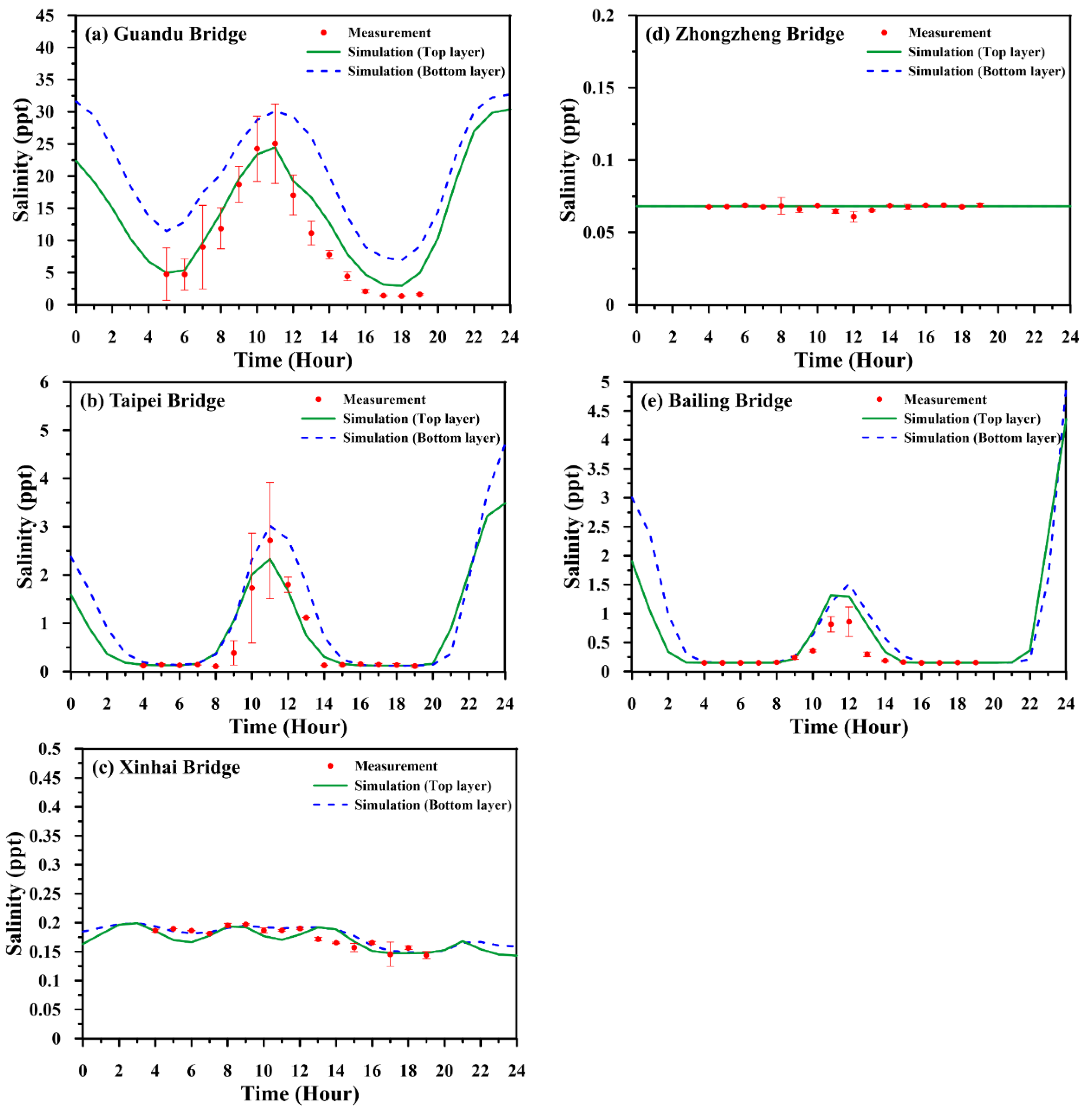
4.2. Model-Data Comparison for Salinity

The salinity data measured on 24 June 2017 were utilized for model-to-data comparisons. Figure 5 displays comparisons between the model simulations and measured salinities at five intensive survey stations. According to this figure, we found that the simulated salinities reasonably reproduced the measured salinities at all stations.

Table 5. Statistical errors between the simulated and measured salinities.

Station	RMSE (ppt)	MAPE (%)	CC	SS	NSE
Guandu Bridge	5.528	114.8	0.963	0.890	0.508
Taipei Bridge	0.292	56.5	0.964	0.970	0.862
Xinhai Bridge	0.011	5.1	0.779	0.882	0.578
Zhongzheng Bridge	0.002	2.1	0.794	0.333	−0.118
Bailing Bridge	0.280	37.4	0.957	0.829	−0.569

shows the statistical errors between the simulated and measured salinities. Based on the SS values, the model performance at Guandu Bridge, Taipei Bridge, Xinhai Bridge, and Bailing Bridge is excellent, while the performance at Zhongzheng Bridge is at the good level. The CC values are above 0.75, which is acceptable. According to the NSEs, the model performances at Zhongzheng Bridge and Bailing Bridge were unsatisfactory. Note that the RMSE and MAPE were higher at Guandu Bridge. The reason could be that the simulations overestimate the observed salinities, possibly due to the underestimated turbulence diffusivity.

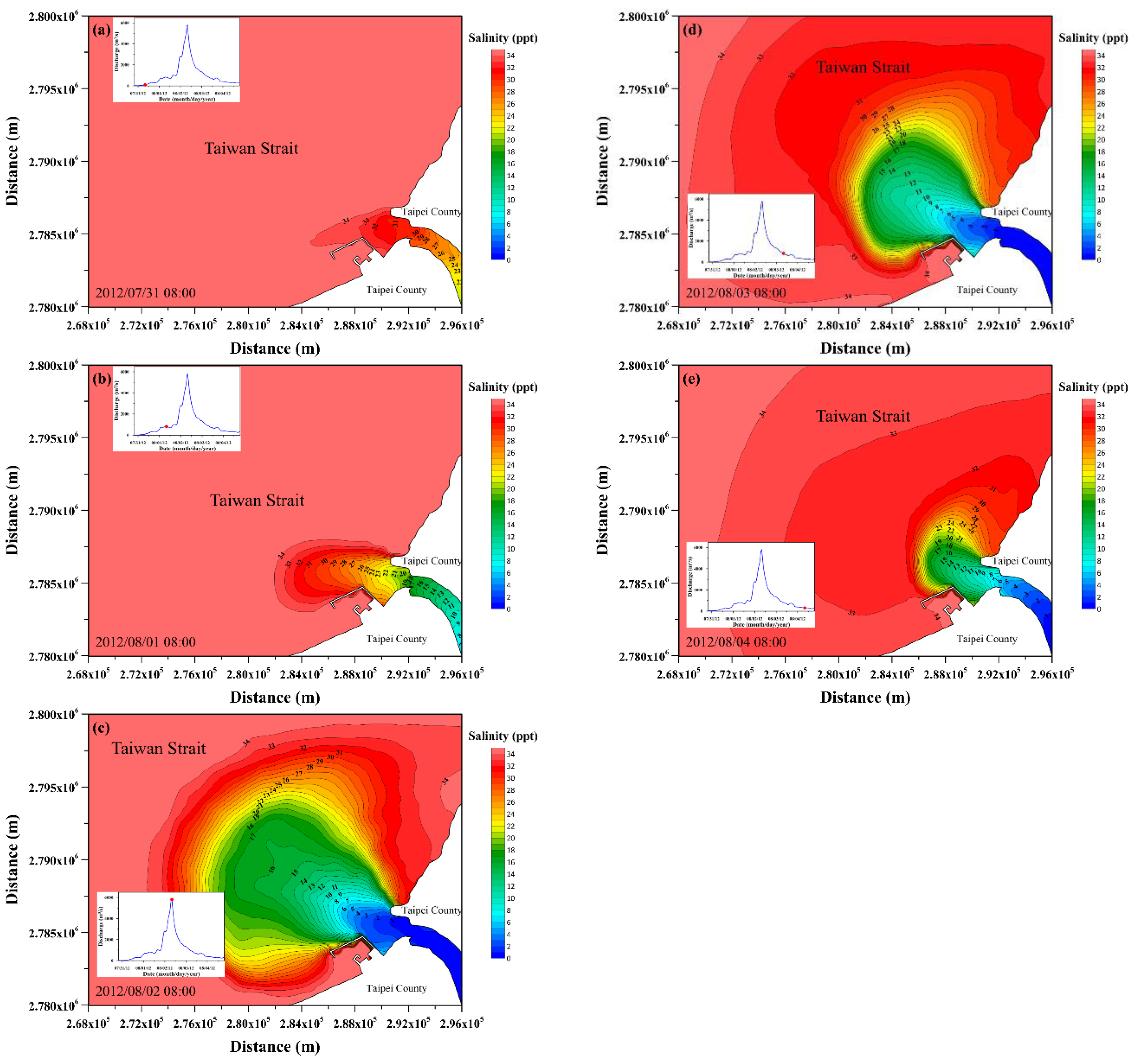
4.3. Effect of Freshwater Discharge

After the model-to-data comparison, the model demonstrated its predictive power. The model was further adopted to examine the influences of freshwater discharges, tides, and winds on the salinity plumes along the continental shelf.

Freshwater discharges from upstream reaches play a crucial role in influencing the buoyant plumes in coastal regions and the recovery times within estuaries. The well-constructed model was employed to investigate the salinity plume at the river mouth under typhoon events and to simultaneously explore the recovery times in the Danshuei River estuary. To drive the model run, five tidal components (e.g., M₂, S₂, N₂, K₁, and O₁) were adopted to produce a time series of the water surface elevations to provide the open boundary conditions at the coastal seas. The freshwater discharges at the upstream boundaries of the three main tributaries during Typhoon Saola, which occurred in 2012, were specified. As Typhoon Saola (2012) was an extreme event, it was considered to represent a real case for analysis. The peak flows during Typhoon Saola at the upstream boundaries of the three tributaries were 1803.9 m³/s, 3249.7 m³/s, and 755.1 m³/s, respectively. The total freshwater discharges from the upstream boundaries are illustrated in Figure 6a. The freshwater discharge levels increased from 30 July and ceased on 3 August 2012 as the typhoon passed northern Taiwan. Normal flows are specified at the upstream boundaries of three main tributaries, which are 4.6 m³/s, 18.5 m³/s, and 2.12 m³/s, respectively.

Figure 6b delineates the time series of the predicted surface salinities with Typhoon Saola and under normal conditions at the Danshuei River mouth. The predicted results were used to estimate the recovery time at the mouth, which was approximately 183 h. Figure 7 shows snapshots of the surface salinity distributions and the insets indicate the corresponding tidal phases. The maximum plume distance from the river mouth and the maximum plume area were 21.7 km and 394.8 km², respectively, which occurred at 08:00 on 3 August. The plume distances and plume areas for the other periods shown in Figure 7 are presented in

Table 6. Plume distances and plume areas for different periods during Typhoon Saola (2012).

Time (Month/Date Hour:Minute)	Plume Distance (km)	Plume Area (km2)
July 31 08:00	3.08	11.51
August 1 08:00	6.82	33.55
August 2 08:00	17.88	283.79
August 3 08:00	21.70	394.80
August 4 08:00	19.13	360.74

. The calculated plume distances and areas are based on the 34 ppt isohaline. These results clearly indicate that the maximum plume distances and areas and peak freshwater discharges (Figure 6a) displayed a time lag of approximately 24 h. The results show that it takes some time for the freshwater discharge inputs from the upstream boundaries to affect the salinity plume. For large tidal estuaries such as Chesapeake Bay and Galveston Bay, the times necessary to recover to normal conditions are on the order of months [54,55]. The recovery times for the Danshuei River estuary and adjacent coast are significantly different by an order of magnitude.

To investigate the relationships between freshwater discharges and plume distances and areas, the freshwater discharges with different exceedance probabilities, listed in Table 1, were specified at the upstream boundaries. Figure 8 shows that the plume distances varied between 4.05 km and 6.9 km, the plume areas varied between 11.32 km² and 37.44 km² over the freshwater discharge range investigated, and the plume distances and plume areas have close to linear relationships with the freshwater discharges. The model results show that the plume distance and plume area increase as the freshwater discharge input increases (Figure 8). Exploring the regression relationships between the plume distance/plume areas and freshwater discharge inputs is useful and predictable to comprehend the hydrological and physical processes within estuaries. The regressions of plume distance (PD)/plume area (PA) versus the total freshwater discharge input (Q) show excellent coefficients of determination (R²), as follows:

$$PD=0.0112\times Q+4.06\hspace{1em}{R}^2=0.99$$

(6)

and

$$PA=0.102\times Q+9.97\hspace{1em}{R}^2=0.99$$

(7)

These two equations could easily be used to estimate the plume distances and plume areas, as the total freshwater discharge inputs were known.

4.4. Effect of Tidal Forcing

Tidal forcing might have a significant influence on tidal mixing and the salinity distributions within estuaries [56,57,58]. To examine the tidal effect on the salinity plume (especially during spring and neap tides), numerical experiments based on the SCHISM with and without tidal actions were conducted. Note that in terms of tidal forcing, the flood (or ebb) tides cause a large amount of seawater to flow into (or out of) the estuary system. In the meantime, the river brings freshwater into the system as well. In other words, the amount of water changes. Thus, a fixed discharge rate (instead of the volume amount) under different tidal conditions was considered for the comparisons in these scenario cases. The mean discharges at the upper reaches of three tributaries, the Dahan, Xindian, and Keelung Rivers, were specified as 29.18 m³/s, 60.84 m³/s, and 26.68 m³/s, respectively. Figure 9 depicts the surface salinity distributions for different tidal conditions, including spring with high and low slack tides (see the left and right subplots in the top panel) and neap with high and low tides (see the left and right subplots in the middle panel). Figure 9e also shows the surface salinity plume without the tidal forcing. When excluding tidal forcing, the salinity plume distances and areas are much larger than those with tidal forcing (

Table 7. Plume distances and plume areas under different tidal forcings and excluding tides.

Tidal Condition	Plume Distance (km)	Plume Area (km2)
Spring with high slack tide	2.24	5.64
Spring with low slack tide	5.78	24.53
Neap with high slack tide	9.09	59.46
Neap with low slack tide	7.24	58.78
Excluding tidal forcing	22.83	400.0

) since salinity plumes are subjected to freshwater discharge inputs only. Figure 9a–d clearly demonstrates the evolution of plume variation under various tidal conditions. The plume distance and area are greatly compressed during the high slack of spring tide (see Figure 9a,b). Later on, with continuous inflows from freshwater and weaker tidal mixing, the maximum plume distance and area (see Figure 9c) on the continental shelf can be found during neap and high slack tides [28,59]. Zhao et al. [10] documented that the salinity plume structures with and without tides were quite similar, which indicated that tidal forcing was not significant in the Wanquan River estuary, China. Vic et al. [60] also demonstrated that tidal forcing did not influence the plume dynamics if the ratio of the tidal amplitude to mouth depth was much smaller. The present study, however, showed that the tidal forcing significantly controlled the salinity plume off the Danshuei River estuary.

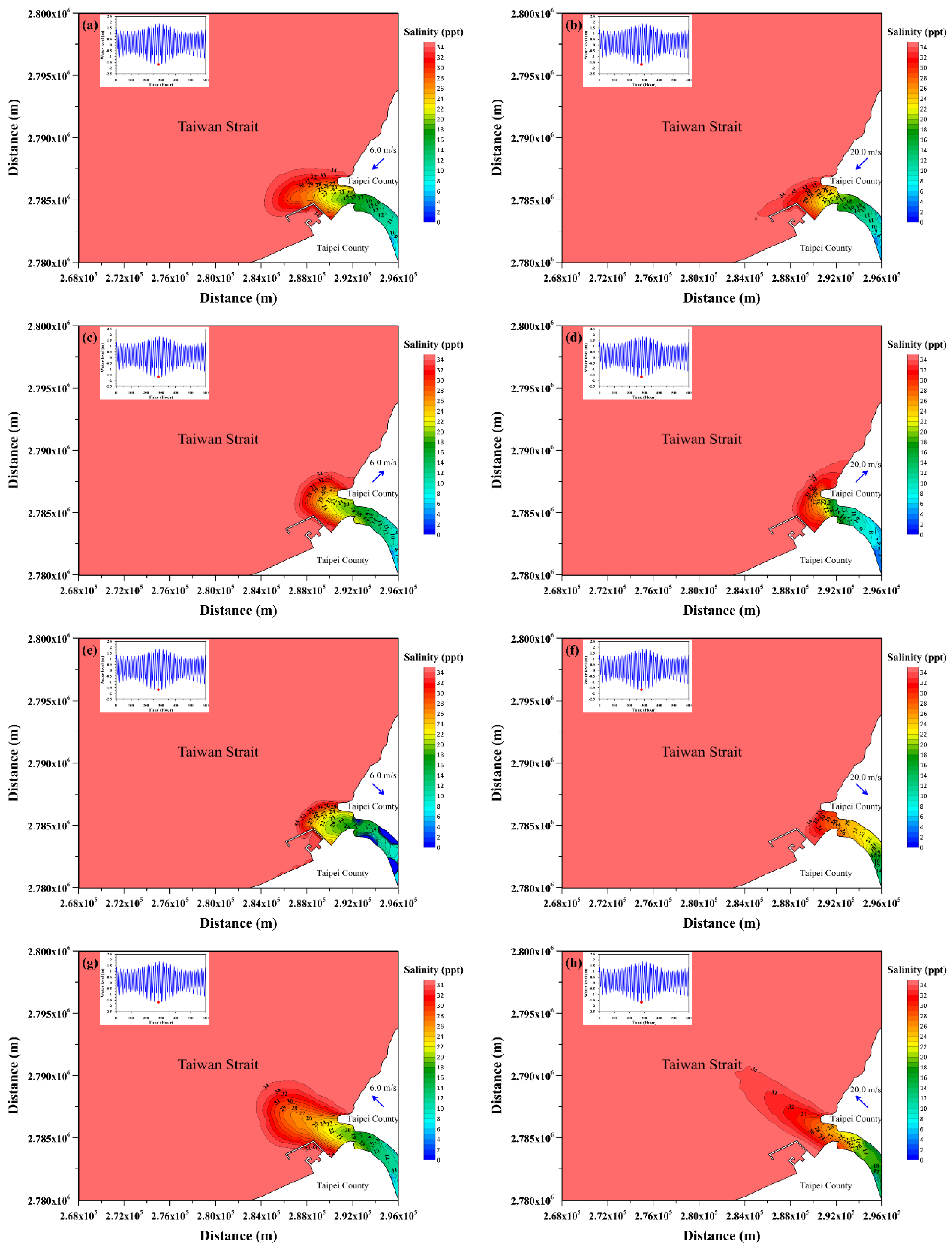
4.5. Effect of Wind Forcing

Wind forcing is also a vital driving factor that affects salinity plumes on continental shelves [30,31,32,35,61]. In the following simulations, the wind stresses, freshwater discharges, and tidal forcings were included in the model simulations. The open boundaries for tidal forcing were specified using the same conditions presented in Section 4.3. The upstream boundaries for the freshwater discharges at the upstream reaches of the three major tributaries were specified using the mean flows (see Section 4.4). According to the annual climatological data report from the Taiwan Center Weather Bureau (2019), northeasterly winds occur during the autumn and winter seasons, while southwesterly winds frequently occur during the spring and summer seasons. Therefore, the wind forcing experiments include two main prevailing wind directions (e.g., northeasterly and southwesterly) as well as two minor wind directions (e.g., northwesterly and southeasterly) with two wind speeds of 6 m/s and 20 m/s. A constant wind persisting over the modeling period was set for all simulations.

Figure 10 depicts the surface salinity distributions during spring low slack tides under northeasterly, southwesterly, northwesterly, and southeasterly winds. The plume distances and areas for different wind speeds and directions are summarized in

Table 8. Plume distances and plume areas for different wind speeds and directions.

Wind Condition	Plume Distance (km)	Plume Area (km2)
6 m/s northeast wind	5.29	21.19
20 m/s northeast wind	3.08	11.17
6 m/s southwest wind	4.59	15.34
20 m/s southwest wind	3.36	12.43
6 m/s northwest wind	3.58	10.61
20 m/s northwest wind	1.73	4.20
6 m/s southeast wind	7.98	31.50
20 m/s southeast wind	9.32	22.82

. It can be seen that southward and northward plumes occur under northeasterly and southwesterly winds (Figure 10a–d), respectively, especially in the high wind (i.e., 20 m/s) condition. Fong and Geyer [62] and Soares et al. [63] also demonstrated that the winds favorable for coastal upwelling and downwelling enhanced the level of vertical stratification to form a narrow plume along the coastline. When the wind blows in an opposite direction (northeasterly), the freshwater is accumulated in the estuary [64]. As a consequence, plume dynamics are hindered with greatly decreased plume distances and areas (Figure 10e,f). In contrast, the southeasterly wind pushing the surface water out of the estuary can enhance the salinity plume, leading to a much larger plume distance and area (Figure 10g,h).

5. Discussion

Freshwater discharge and wind stress are two critical factors that influence river plumes in coastal regions [65]. To determine which is the most dominant factor, we used the Wedderburn number (W), which is a dimensionless parameter used to indicate the relative strengths of freshwater discharges and wind stresses acting on river plumes [21,66,67]. The Wedderburn number can be written as follows:

$$W=\frac{{\tau }_w\ell }{\Delta \rho g{h}^2}$$

(8)

where g denotes the gravitational acceleration, h represents the section-averaged plume depth, $\ell$ expresses the distance from the river mouth to the offshore boundary of the river plume, ${\tau }_w$ indicates the wind stress, and $\mathrm{\Delta }\rho$ denotes the density variation over $\ell$. If W > 1, the river plume is controlled by the wind stress, which can dominate the flow direction and plume stratification. If W < 1, the river plume is controlled by freshwater discharge, which can dominate the plume structure.

Table 9. Wedderburn numbers under different wind speeds and directions and freshwater discharges from the upstream reaches.

Freshwater Discharge Condition	Wedderburn Number (W)
	6 m/s Northeast Wind	20 m/s Northeast Wind	6 m/s Southwest Wind	20 m/s Southwest Wind	6 m/s Northwest Wind	20 m/s Northwest Wind	6 m/s Southeast Wind	20 m/s Southeast Wind
Q10	0.083	0.612	0.064	0.155	0.028	0.293	0.143	2.423
Q20	0.084	0.991	0.072	0.162	0.029	0.309	0.156	3.082
Q30	0.102	1.226	0.100	0.179	0.030	0.319	0.172	3.191
Q40	0.113	1.334	0.105	0.194	0.032	0.345	0.187	3.698
Q50	0.117	1.507	0.106	0.210	0.037	0.387	0.192	3.906
Q60	0.119	1.656	0.116	0.226	0.040	0.420	0.200	3.946
Q70	0.134	1.836	0.121	0.240	0.045	0.460	0.215	4.198
Q80	0.141	1.903	0.124	0.324	0.045	0.481	0.220	4.454
Q90	0.142	2.193	0.135	0.346	0.050	0.527	0.226	5.125

shows the calculated Wedderburn number (W) values for different wind speeds and directions and freshwater discharges. The results shown here clearly indicate that when the wind speeds increase or the freshwater discharges decrease, the W value increases. When the wind speeds are 6 m/s and 20 m/s for both the southwest and northwest directions, the plume is dominated by freshwater discharges (W < 1). When the wind speed is 6 m/s for both the northeast and southeast directions, the plume is also controlled by freshwater discharges. When the freshwater discharges decrease from Q₃₀ to Q₉₀ flows and the wind speed is 20 m/s in the northeast direction, wind forcing dominates the river plume (W > 1). Regardless of the level of freshwater discharge, the wind speed is 20 m/s in the southeast direction, and the W value is greater than 1. This is because the wind direction is the same as that of the plume. Conversely, when the wind speed is 20/s and northwesterly winds flow upstream of the Danshuei River against the plume, these conditions do not assist the river plume in diffusing water. Therefore, the W value is less than 1, and the plume is dominated by freshwater discharge.

The Danshuei River estuary has been subjected to severe pollution, which consists of organic and inorganic nutrients, heavy metals, suspended sediment, and fecal coliform bacteria [68]. In summer, due to the low flows and high temperatures, the dissolved oxygen concentrations in the water column are less than 2 mg/L [69], which causes fish death. Transporting pollutants offshore by river plumes is even more important. Based on the calculations of the W values, the freshwater discharges dominate the river plume, and the secondary forcing comes from wind. Controlling freshwater discharges upstream of the three tributaries and reservoirs to dilute pollutants and carry them offshore by river plumes is a crucial issue that the government should consider.

6. Conclusions

A 3D circulation model, SCHISM, was employed to explore the river plumes offshore from the Danshuei River and the recovery times in tidal estuaries. The model was constructed and validated against the measured hydrodynamic and salinity data. The results indicate that the simulations reasonably reproduced the measured tidal amplitudes and phases, tidal velocities, and salinity data. The validated model was used to estimate the recoveries during typhoon events and to explore the effects of freshwater discharges, tidal forcing, and wind forcing on river plume dispersal.

The salinity recovery time is an effective timescale to respond to high flows during typhoon events. The salinity recovery time at the mouth of the Danshuei River was approximately 183 h for Typhoon Saola in 2012. A linear regression relationship between plume distances/plume areas and total freshwater discharge inputs was identified. Compared to the simulated results with and without tidal forcing, the salinity plume distances and plume areas with the exclusion of tidal forcing were larger than those with tidal forcing. This numerical experiment reveals that tidal forcing plays an important role in affecting the salinity plume. Obviously, the southward and northward plumes are accompanied by northeasterly winds and southwesterly winds, respectively, especially for strong winds. Based on the calculated Wedderburn number (W) values, we found that freshwater discharges mainly dominated the river plume offshore. The controlling freshwater discharges from the upstream reaches of the three tributaries and two reservoirs in the Xindian River and Dahan River significantly influence the river plume and transport pollutants offshore, which reduces the pollution concentrations in tidal estuaries.

In future studies, the SCHISM-based model will be improved to combine the water quality and ecosystems, fecal coliform bacteria data, and heavy metal modules to predict the contaminant transport in tidal estuaries and to explore contaminant plumes offshore.

References

1. Falcieri, F.M.; Benetazzo, A.; Sclavo, M.; Russo, A.; Carniel, S. Po River plume variability investigated from model data. Cont. Shelf Res. 2014, 87, 84–95. [Google Scholar] [CrossRef]
2. Rippy, M.A.; Stein, R.; Sanders, B.F.; Davis, K.; McLaughlin, K.; Skinner, J.F.; Kappeler, J.; Grant, S.B. Small drains, big problems: The impact of dry weather runoff on shoreline water quality at enclosed beaches. Environ. Sci. Technol. 2014, 48, 14168–14177. [Google Scholar] [CrossRef] [PubMed] [Green Version]
3. Tao, H.Y.; Leonardi, N.; Li, J.F.; Fagherazzi, S. Sediment transport in a surface-advected estuarine plume. Cont. Shelf Res. 2016, 116, 122–135. [Google Scholar]
4. Xu, C.; Xu, Y.; Hu, J.; Li, S.; Wang, B. A numerical analysis of the summertime Pearl River plume from 1999 to 2010: Dispersal patterns and intraseasonal variability. J. Mar. Syst. 2019, 192, 15–27. [Google Scholar] [CrossRef]
5. Gong, W.; Chen, L.; Chen, Z.; Zhang, H. Plume-to-plume interactions in the Pearl River Delta in winter. Ocean Coast. Manag. 2019, 175, 110–126. [Google Scholar] [CrossRef]
6. Zhang, Y.; Li, D.; Wang, K.; Xue, B. Contribution of biological effects to the carbon sources/sinks and the tropic status of the ecosystem in the Changjiang (Yangtze) River Estuary plume in summer as indicated by net ecosystem production variations. Water 2019, 11, 1264. [Google Scholar] [CrossRef] [Green Version]
7. Gao, N.; Ma, Y.; Zhao, M.; Zhang, L.; Zhan, H.; Cai, S.; He, Q. Quantile analysis of long-term trends of near-surface chlorophyll-a in the Pearl River plume. Water 2020, 12, 1662. [Google Scholar] [CrossRef]
8. Kamidis, N.; Sylaios, G.; Tsihrintzis, V.A. Modeling the Nestos River plume dynamics using ELCOM. Desalin. Water Treat. 2011, 33, 22–35. [Google Scholar] [CrossRef]
9. Wang, B.; Hirose, N.; Yuan, D.; Moon, J.H.; Pan, X. Effects of tides on cross-isobath movement of the low-salinity plume in the western Yellow and East China Seas in winter. Cont. Shelf Res. 2017, 143, 228–239. [Google Scholar] [CrossRef]
10. Zhao, J.; Gong, W.; Shen, J. The effect of wind on the dispersal of a tropical small river plume. Front. Earth Sci. 2018, 12, 170–190. [Google Scholar] [CrossRef]
11. Couveia, N.A.; Gherardi, D.F.; Wagner, F.H.; Paes, E.T.; Coles, V.J.; Aragao, L.E.O.C. The salinity structure of the Amazon River plume drives spatiotemporal variation of oceanic primary productivity. J. Geophy. Res. Biogeosci. 2019, 124, 147–165. [Google Scholar]
12. Kourafalou, V.H. River plume development in semi-enclosed Mediterranean regions: North Adriatic Sea and Northwestern Aegean Sea. J. Mar. Syst. 2001, 30, 181–205. [Google Scholar] [CrossRef]
13. Garvine, R.W. Penetration of a buoyant coastal discharge onto the continental shelf: A numerical model experiment. J. Phys. Oceanogr. 1999, 29, 1892–1909. [Google Scholar] [CrossRef]
14. Tseng, Y.H.; Bryan, F.O.; Whitney, M.M. Impacts of the representation of riverine freshwater input in the community earth system model. Ocean Model. 2016, 105, 71–86. [Google Scholar] [CrossRef] [Green Version]
15. Lee, J.H.; Moon, I.J.; Moon, J.H.; Kim, S.H.; Jeong, Y.Y.; Koo, J.H. Impact of typhoons on the Changjiang plume extension in the Yellow and East China Seas. J. Geophy. Res. Ocean. 2017, 122, 4962–4973. [Google Scholar] [CrossRef]
16. Sasmal, K.; Masunaga, E.; Webb, A.; Fringer, O.B.; Gross, E.S.; Rayson, M.D.; Yamazaki, H. A three-dimensional numerical study of river plume mixing processes in Otsuchi Bay, Japan. J. Oceanogr. 2018, 74, 169–186. [Google Scholar] [CrossRef]
17. Dumasdelage, R.; Delestre, O. Simulating coliform transport and decay from 3D hydrodynamics model and in situ observation in Nice area. SN Appl. Sci. 2020, 2, 1348. [Google Scholar] [CrossRef]
18. Hopkins, J.; Lucas, M.; Dufau, C.; Sutton, M.; Stum, J.; Lauret, O.; Channelliere, C. Detection and variability of the Congo River plume from satellite derived sea surface temperature, salinity, ocean colour and sea level. Remote Sen. Environ. 2013, 139, 365–385. [Google Scholar] [CrossRef]
19. Liao, X.; Du, Y.; Wang, T.; Hu, S.; Zhan, H.; Liu, H.; Wu, G. High-frequency variations in Pearl River plume observed by soil moisture active passive seas surface salinity. Remote Sens. 2020, 12, 563. [Google Scholar] [CrossRef] [Green Version]
20. Phillipson, L.; Toumi, R. Assimilation of satellite salinity for modelling the Congo River plume. Remote Sens. 2020, 12, 11. [Google Scholar] [CrossRef] [Green Version]
21. Dzwonkowski, B.; Park, K.; Collini, R. The coupled estuarine-shelf response of a river-dominated system during the transition from low to high dicharge. J. Geophys. Res. Ocean. 2015, 120, 6145–6163. [Google Scholar] [CrossRef] [Green Version]
22. Horner-Devine, A.R.; Pietrzak, J.D.; Souza, A.J.; McKeon, M.A.; Meirelles, S.; Henriquez, M.; Flores, R.P.; Rijnsburger, S. Cross-shore transport of nearshore sediment by river plume frontal pumping. Geophys. Res. Lett. 2017, 44, 6343–6351. [Google Scholar] [CrossRef] [Green Version]
23. Mulligan, R.P.; Perrie, W. Circulation and structure of the Mackenzie River plume in the coastal Arctic Ocean. Cont. Shelf Res. 2019, 177, 59–68. [Google Scholar] [CrossRef]
24. Chao, S.Y. Wind-driven motion of estuarine plumes. J. Phys. Oceanogr. 1988, 18, 1144–1166. [Google Scholar] [CrossRef] [Green Version]
25. Chao, S.Y. Tidal modulation by estuarine plumes. J. Phys. Oceanogr. 1990, 20, 1115–1123. [Google Scholar] [CrossRef] [Green Version]
26. Hetland, R.D. Relating river plume structure to vertical mixing. J. Phys. Oceanogr. 2005, 35, 1667–1688. [Google Scholar] [CrossRef]
27. Shi, J.Z.; Lu, L.F.; Liu, Y.N. The hydrodynamics of an idealized estuarine plume along a straight coast: A numerical study. Environ. Model. Assess. 2010, 15, 487–502. [Google Scholar] [CrossRef]
28. Rong, Z.; Li, M. Tidal effects on bulge region of Changjiang River plume. Estuar. Coast. Shelf Sci. 2012, 97, 149–160. [Google Scholar] [CrossRef]
29. Osadchiev, A.A.; Zavialov, P.O. Lagrangian model of a surface-advected river plume. Conti. Shelf Res. 2013, 58, 96–106. [Google Scholar] [CrossRef]
30. Sousa, M.C.; Vaz, N.; Alvarez, I.; Gomez-Gesteira, M.; Dias, J.M. Modeling the Minho River plume intrusion into the Rias Baixas (NW Iberian Peninsula). Cont. Shelf Res. 2014, 85, 30–41. [Google Scholar] [CrossRef]
31. Zheng, S.; Guan, W.; Cai, S.; Wei, X.; Huang, D. A model study of the effects of river discharges and interannual variation of winds on the plume front on winter in Pear River Estuary. Cont. Shelf Res. 2014, 73, 31–40. [Google Scholar] [CrossRef]
32. Androulidakis, Y.S.; Kourafalou, V.H.; Schiller, R.V. Process studies on the evolution of the Mississippi River plume: Impact of topography, wind and discharge conditions. Cont. Shelf Res. 2015, 107, 33–49. [Google Scholar] [CrossRef] [Green Version]
33. Hong, J.S.; Moon, J.H.; Lee, J.H.; Pang, I.C. Modeling the largest inflow of Changjiang freshwater into the Yellow Sea in 2012 with particle-tracking experiment. Ocean Sci. J. 2016, 51, 549–562. [Google Scholar] [CrossRef]
34. Ping, Z.; Hui, W. Origins and transports of the low-salinity coastal water in the southwestern Yellow Sea. Acta Oceanol. Sin. 2018, 37, 1–11. [Google Scholar]
35. Yu, X.; Guo, X.; Morimoto, A.; Buranapratheprat, A. Simulation of river plume behaviors in a tropical region: Case study of the Upper Gulf of Thailand. Cont. Shelf Res. 2018, 153, 16–29. [Google Scholar] [CrossRef]
36. Des, M.; deCastro, M.; Sousa, M.G.; Dias, J.M.; Gomez-Gesteria, M. Hydrodynamics of river plume intrusion into an adjacent estuary: The Minho River and Ria de Vigo. J. Mar. Syst. 2019, 189, 87–97. [Google Scholar] [CrossRef]
37. Fu, B.; Horsburgh, J.S.; Jakeman, A.J.; Gualtieri, C.; Arnold, T.; Marshall, L.; Green, T.R.; Quinn, N.W.T.; Volk, M.; Hunt, R.J.; et al. Modeling water quality in watersheds: From here to the next generation. Water Resour. Res. 2020, 56, e2020WR027721. [Google Scholar] [CrossRef]
38. Chen, W.B.; Liu, W.C.; Hsu, M.H. Water quality modeling in a tidal estuarine system using a three-dimensional model. Environ. Eng. Sci. 2011, 28, 443–459. [Google Scholar] [CrossRef]
39. Water Resources Agency. Hydrological and Hydrodynamic Verification Report of the Danshuei River System. 2018. Available online: https://www-ws.wra.gov.tw/Download.ashx?u=LzAwMS9VcGxvYWQvNDIzL3JlbGZpbGUvMC8yMzkxOC8yZTk0MDU3YS0xOTExLTQ1YWYtOGZjMC0xZTA3ODE4MzMwYjIucGRm&n=MTA35reh5rC05rKz5rC057O75rC05paH5rC055CG6KuW6K2J5aCx5ZGKLnBkZg%3D%3D (accessed on 1 December 2021).
40. Hsu, M.H.; Kuo, A.Y.; Kuo, J.T.; Liu, W.C. Procedure to calibrate and verify numerical models of estuarine hydrodynamics. J. Hydrau. Eng. 1999, 125, 166–182. [Google Scholar] [CrossRef]
41. Liu, W.C.; Chen, W.B.; Kuo, J.T. Modeling residence time response to freshwater discharge in a mesotidal estuary, Taiwan. J. Mar. Syst. 2008, 74, 295–314. [Google Scholar] [CrossRef]
42. Liu, W.C. Modelling circulation and vertical mixing in estuaries. Proc. Inst. Civil Eng. Marit. Eng. 2006, 159, 67–76. [Google Scholar] [CrossRef]
43. Zhang, Y.J.; Ateljevich, E.; Yu, H.C.; Wu, C.H.; Yu, J.C.S. A new vertical coordinate system for a 3D unstructured-grid model. Ocean Model. 2015, 85, 16–31. [Google Scholar] [CrossRef]
44. Zhang, Y.J.; Ye, F.; Stanev, E.V.; Grashorn, S. Seamless cross-scale modeling with SCHISM. Ocean Model. 2016, 102, 64–81. [Google Scholar] [CrossRef] [Green Version]
45. Zhang, Y.L.; Baptista, A.M. SELFE: A semi-implicit Eulerian-Lagrangian finite-element model for cross-scale ocean circulation. Ocean Model. 2008, 21, 71–96. [Google Scholar] [CrossRef]
46. Kantha, L.H.; Clayson, C.A. An improved mixed layer model for geophysical applications. J. Geophys. Res. 1994, 99, 25235–25266. [Google Scholar] [CrossRef]
47. Umlauf, L.; Burchard, H. A generic length-scale equation for geophysical turbulence models. J. Mar. Res. 2003, 61, 235–265. [Google Scholar] [CrossRef]
48. Ye, F.; Zhang, Y.J.; Wang, H.V.; Friedrichs, M.A.M.; Irby, I.D.; Alteljevich, E.; Valle-Levinson, A.; Wang, Z.; Huang, H.; Shen, J.; et al. A 3D unstructured-grid model for Chesapeake Bay: Important of bathymetry. Ocean Model. 2018, 127, 16–39. [Google Scholar] [CrossRef] [Green Version]
49. Egbert, G.D.; Erofeeva, S.Y. Efficient inverse modeling of barotropic ocean tides. J. Atmos. Ocean. Technol. 2002, 19, 183–204. [Google Scholar] [CrossRef] [Green Version]
50. Bennett, N.D.; Croke, B.F.W.; Guariso, G.; Guillaume, J.H.A.; Hamilton, S.H.; Jakeman, J.A.; Marsili-Libelli, S.; Newham, L.T.H.; Norton, J.P.; Perrin, C.; et al. Characterising performance of environmental models. Environ. Model. Softw. 2013, 40, 1–20. [Google Scholar] [CrossRef]
51. Willmott, C.J. On the validation of models. Phys. Geogr. 1981, 2, 184–194. [Google Scholar] [CrossRef]
52. Nash, J.E.; Sutcliffe, J.V. River flow forecasting through conceptual models, part I-a discussion of principles. J. Hydrol. 1970, 10, 282–290. [Google Scholar] [CrossRef]
53. Chen, W.; Chen, K.; Kuang, C.; Zhu, D.Z.; He, L.; Mao, X.; Liang, H.; Song, H. Influence of sea level rise on saline water intrusion in the Yangtz River Estuary. Appl. Ocean Res. 2016, 54, 12–25. [Google Scholar] [CrossRef]
54. Nichols, M. Response of coastal plain estuaries to episodic events in the Chesapeake Bay region. In Nearshore and Estuarine Cohesive Sediment Transport, Mehta, A., Ed.; Springer: Berlin, Germany, 1993; pp. 1–20. [Google Scholar]
55. Du, J.; Park, K. Estuarine salinity recovery from an extreme precipitation event: Hurricane Harvey in Galveston Bay. Sci. Total Environ. 2019, 670, 1049–1059. [Google Scholar] [CrossRef] [PubMed]
56. Uncles, R.J.; Stephens, J.A. The effect of wind, runoff and tides on salinity in a strongly tidal sub-estuary. Estuar. Coast. 2011, 34, 758–774. [Google Scholar] [CrossRef]
57. Gong, W.; Shen, J. The response of salt intrusion to changes in river discharge and tidal mixing during the dry season in the Modaomen Estuary, China. Cont. Shelf Res. 2011, 31, 769–788. [Google Scholar] [CrossRef]
58. Lai, W.; Pan, J.; Devlin, A.T. Impacts of tides and winds on estuarine circulation in the Pearl River Estuary. Conti. Shelf Res. 2018, 168, 68–82. [Google Scholar] [CrossRef]
59. Chen, W.B.; Liu, W.C. Modeling investigation of asymmetric tidal mixing and residual circulation in a partially stratified estuary. Environ. Fluid Mech. 2015, 16, 167–191. [Google Scholar] [CrossRef]
60. Vic, C.; Berger, H.; Treguier, A.M.; Couvelard, X. Dynamics of an equatorial river plume: Theory and numerical experiments applied to congo plume case. J. Phys. Oceanogr. 2014, 44, 980–994. [Google Scholar] [CrossRef] [Green Version]
61. Pargaonkar, S.M.; Vinayachandran, P.N. Wind forcing of the Ganga-Brahmaputra river plume. Ocean Dynam. 2021, 71, 125–156. [Google Scholar] [CrossRef]
62. Fong, D.A.; Geyer, W.R. The alongshore transport of freshwater in a surface-trapped river plume. J. Phys. Oceanogr. 2002, 32, 957–972. [Google Scholar] [CrossRef]
63. Soares, I.D.; Kourafalou, V.; Lee, T.N. Circulation on the western South Atlantic continental shelf. Part 2: Spring and autumn realistic simulations. J. Geophys. Res. 2007, 112, C04003. [Google Scholar]
64. Choi, B.J.; Wilkin, J.L. The effect of wind on the dispersal of the Hudson River plume. J. Phys. Oceanogr. 2007, 37, 1878–1897. [Google Scholar] [CrossRef]
65. Zhang, H.; Hu, S.; Cheng, W.; Zhu, L.; Chen, Y.; Liu, J.; Gong, W.; Li, Y.; Li, S. Response of freshwater transport during typhoons with wave-induced mixing effects in Pearl River Estuary, China. Estuar. Coast. Shelf Sci. 2021, 258, 107439. [Google Scholar] [CrossRef]
66. Chen, S.N.; Sanford, L.P. Axial wind effects on stratification and longitudinal salt transport in an idealized, partially mixed estuary. J. Phys. Oceanogr. 2009, 39, 1905–1920. [Google Scholar] [CrossRef]
67. Jurisa, J.T.; Chant, R. The coupled Hudson River estuarine-plume response to variable wind and river forcings. Ocean Dynam. 2012, 62, 771–784. [Google Scholar] [CrossRef]
68. Liu, W.C.; Liu, H.M.; Ken, P.J. Investigating the contaminant transport of heavy metals in estuarine waters. Environ. Monit. Assess. 2020, 192, 32. [Google Scholar] [CrossRef]
69. Liu, W.C.; Liu, S.Y.; Hsu, M.H.; Kuo, A.Y. Water quality modeling to determine minimum instream flow for fish survival in tidal rivers. J. Environ. Manag. 2005, 76, 293–308. [Google Scholar] [CrossRef]
Figure 1. (a) Map of the Danshuei River estuarine system including the Danshui River–Dahan River, Xindian River, and Keelung River and the adjacent coastal seas, and (b) unstructured grid of the horizontal dimensions in the computational domain for the SCHISM model simulations.
Water 14 00429 g001
Figure 2. Comparison of the simulated and measured tidal amplitudes, including M2, S2, N2, K1, and O1, at the (a) Danshuei River mouth, (b) Taipei Bridge, (c) Xinhai Bridge, (d) Zhongzheng Bridge, and (e) Bailing Bridge.
Water 14 00429 g002
Figure 3. Comparison of the simulated and measured phases, including M2, S2, N2, K1, and O1, at the (a) Danshuei River mouth, (b) Taipei Bridge, (c) Xinhai Bridge, (d) Zhongzheng Bridge, and (e) Bailing Bridge.
Water 14 00429 g003
Figure 4. Comparisons of the simulated and measured tidal currents on 24 June 2017 at the (a) Guandu Bridge, (b) Taipei Bridge, (c) Xinhai Bridge, (d) Zhongzheng Bridge, and (e) Bailing Bridge.
Water 14 00429 g004
Figure 5. Comparisons of the simulated and measured salinities on 24 June 2017 at the (a) Guandu Bridge, (b) Taipei Bridge, (c) Xinhai Bridge, (d) Zhongzheng Bridge, and (e) Bailing Bridge.
Water 14 00429 g005
Figure 6. (a) Total freshwater discharge inputs from the upstream reaches of the Dahan River, Xindian River, and Keelung River during Typhoon Saola in 2012, and (b) time series salinity responses at the Danshuei River mouth to typhoon events (high flow) and normal flow conditions.
Water 14 00429 g006
Figure 7. Snapshots of the surface salinity distributions during Typhoon Saola in 2012 for different periods: (a) 08:00 July 31, (b) 08:00 August 1, (c) 08:00 August 2, (d) 08:00 August 3, and (e) 08:00 August 4.
Water 14 00429 g007
Figure 8. Correlations between (a) plume lengths and (b) plume areas and total freshwater discharges from upstream boundaries.
Water 14 00429 g008
Figure 9. Surface salinity distributions under mean flow conditions for different tidal actions: (a) spring tide with high slack tide, (b) spring tide with low slack tide, (c) neap tide with high slack tide, (d) neap tide with low slack tide, and (e) without tidal effects.
Water 14 00429 g009
Figure 10. Surface salinity distributions under mean flow conditions for different wind speeds and directions: (a) 6 m/s northeast wind, (b) 20 m/s northeast wind, (c) 6 m/s southwest wind, (d) 20 m/s southwest wind, (e) 6 m/s northwest wind, (f) 20 northwest wind, (g) 6 m/s southeast wind, and (h) 20 m/s southeast wind.
Water 14 00429 g010