Smoothed Particle Hydrodynamics Simulations of Porous Medium Flow Using Ergun’s Fixed-Bed Equation

Abstract

A popular equation that is often employed to represent the relationship between the pressure loss and the fluid flow in fluidized or packed granular beds is the Ergun equation, which is an extension of Darcy’s law. In this paper, the method of Smoothed Particle Hydrodynamics (SPH) is used to numerically study the flow field across a rectangular channel partially filled with a porous layer both at the Representative Elementary Volume (REV) scale using the Ergun equation and at the pore scale. Since the flow field can be estimated at the REV scale with a much lower cost compared to the pore scale, it is important to evaluate how accurately the pore-scale results can be reproduced at the REV scale. The comparison between both scales is made in terms of the velocity profiles at the outlet of the rectangular channel and the pressure losses across the clear and porous zones for three different arrays of solid grains at the pore scale. The results show that minimum differences in the flow structure and velocity profiles between the REV and the pore scale always occur at intermediate values of the porosity ($\varphi =0.44$ and 0.55). As the porosity increases, the differences between the REV and the pore scale also increase. The details of the pressure losses are affected by the geometry of the porous medium. In particular, we find that the pressure profiles at the REV scale match those at the pore scale almost independently of the porosity only when the grains are uniformly distributed in a non-staggered square array.

1. Introduction

Fluid flow in porous media has been the subject of active research in the last forty years. It happens frequently in geophysical flows as well as in a countless number of engineering applications, such as enhanced oil recovery, carbon dioxide sequestration, water soil infiltration, water filtering, in the design of packed bed reactors, and in many large-scale chemical processes just to mention a few [1,2,3]. At the pore scale, the movement of solutes in porous materials occurs within an intricate system of interconnected channels or gaps. In highly heterogeneous porous media, the fluid flows through tortuous paths characterized by multiple twists, bends and turns. The combination of Darcy’s law and the principle of mass conservation has frequently been employed to explain the fluid flow through a porous medium [4]. The relationship between energy and flow rate is the most important problem in fluid mechanics when dealing with flow through porous media, and Darcy’s law is the most basic law that describes this relationship [3]. While the Darcy model is only valid for laminar flows, other semi-empirical models such as the Brinkman–Darcy and the Forchheimer–Darcy models were introduced in the literature. In particular, the Brinkman–Darcy model uses an extra viscous term, called the Brinkman term, which allows the description of the flow through porous media with a porosity higher than 90% [5,6]. On the other hand, the Forchheimer–Darcy model was developed to encompass the regions beyond Darcy flow by incorporating a quadratic velocity term. This term accommodates the non-linear relationship between the pressure gradient and velocity [7,8].

Numerical investigations concerning fluid flow in porous media typically encompass two distinct scales, namely the pore scale and the Representative Elementary Volume (REV) scale. Pore-scale simulations of porous media are relatively novel. In this scale, the porous medium characteristics are reconstructed in order to obtain representative pore and solid matrix structures in the numerical models [9,10,11,12,13,14,15,16]. All of these numerical investigations were conducted utilizing conventional computational fluid dynamics (CFD) methods, such as finite-difference or finite-volume formulations. In contrast to the pore scale, the REV-scale approach does not require the explicit reconstruction of the porous medium’s intricate details. Instead, the presence of the porous medium is accounted for by introducing a resistance term into the momentum equation [17,18,19,20,21,22,23,24]. This translates into a low cost of time compared to most pore-scale simulations by guaranteeing a comparable accuracy. However, most of these simulations have relied on lattice Boltzmann methods to deal with the complex fluid–solid boundaries in the intricate structure of the porous medium. For example, Ergun’s equation has recently been applied to model numerically the effects of heat transfer of Cu–water nanofluid through a partially porous wavy channel in the presence of a magnetic field [25] and the magnetohydrodynamical natural convection around a permeable triangular cylinder inside a square enclosure filled with an Al${}_2$O${}_3$–H${}_2$O nanofluid [26].

The flow of fluids through porous media and packed beds of granular solids is subjected to pressure losses due to the simultaneous action of viscous and kinetic energy losses. In the REV-scale approach, the most commonly used equation for calculating the pressure drop has been proposed by Ergun [27]. This equation provides a good basis for estimating the fixed-bed head losses under laminar flow conditions and at rates where the Reynolds number is in the intermediate and turbulent range. It is also quite suitable for determining the flow resistance in packed beds with porosity in the range between 0.4 and 0.6 [28]. Ergun’s equation has been extended to describe metal foams, which possess distinct characteristics compared to packed beds, including significantly higher porosity (≳90%) and a unique complex open-celled cellular structure. Specifically, a granular Representative Unit Cell model applicable to all porosities was developed to address these features. For example, du Plessis et al. [29] described the flow of a Newtonian fluid through a packed bed of uniformly sized spherical granules. Moreover, Bazmi et al. [30] modified the Ergun equation for predicting the pressure losses in trickle bed reactors randomly packed with trilobe particles. More recently, a modification of the standard Ergun equation by multiplying it with a resistance correction coefficient was proposed by Lai et al. [31] to calculate head losses through a high-porosity, open-cell structured porous medium in a rectangular channel. In a more recent study conducted by Pang et al. [32], the intrinsic permeability of crushed coal medium was experimentally determined using the Ergun equation. This research offers valuable insights into the permeability characteristics of the media within fractured coal bodies. An evaluation of the pressure drop in heterogeneous alternating-layer packed beds was modeled by Li et al. [33] using a coupled LES-LBM-IMB-DEM method to obtain the interphase closure of fluid-solid systems. A discrete element method was also applied by Li et al. [34] to evaluate pressure losses in heterogeneous alternating-layer beds for low-carbon operating blast furnaces.

The aforementioned numerical investigations were carried out utilizing conventional computational fluid dynamics (CFD) schemes, including finite difference, finite volume, and lattice Boltzmann formulations. However, in this paper, the authors employ the Smoothed Particle Hydrodynamics (SPH) method, which was initially developed by Lucy [35] and Gingold and Monaghan [36] for the simulation of astrophysical flows, to study the fluid flow through porous media in the REV scale. The SPH method is a Lagrangian scheme that relies on particle interpolation to calculate smooth field variables [37,38]. Since its inception, SPH has become very popular because of its ever-increasing applications to fluid and solid mechanics, among many other fields of science and engineering [39]. Although the SPH method is relatively novel compared to more traditional mesh-based schemes, it is not new to flow modeling in porous media [40,41]. However, most SPH simulations of flow through porous media have been designed using the pore-scale approach [42,43,44,45,46,47]. For example, Jiang et al. [42] employed SPH techniques to simulate fluid flow in isotropic porous media. These authors employed SPH methods and resolved the porous structure at a mesoscopic level by randomly assigning a portion of the SPH particles to fixed locations, while Tartakovsky et al. [43] simulated numerically the fluid flow through anisotropic and heterogeneous porous media. Multiphase flows in porous media with SPH were also modeled by Tartakovsky et al. [44], Kunz et al. [45] and Peng et al. [47] using the pore-scale approach. SPH models of fluid flowing through a deformable porous medium were reported by Lenaerts et al. [48] and Bui and Nguyen [49]. These researchers conducted simulations of porous flow on a macroscopic scale by abstracting individual pores or cavities within the material. On the other hand, the scheme introduced by the latter authors is based on Biot’s two-phase mixture theory. In this scheme, the solid matrix is represented as an elasto-plastic material, while the pore fluid is modeled as an incompressible fluid. SPH simulations of fluid flow through fractured porous media were also recently reported by Shigorina et al. [50] and by Bui and Nguyen [51].

As far as we know, there are no reports in the literature on the SPH modeling of flow in porous media at the REV scale. Since SPH is a Lagrangian scheme, it presents some advantages over traditional Eulerian mesh-based methods in that fluid advection is performed exactly. On the other hand, including more physics to the model is a straightforward task compared to other schemes. Although the pore-scale approach appears to be more accurate and allows studying microscopic seepage and fluid–solid interactions, for large porous systems, it involves a much higher computational cost. Therefore, exploring the ability of SPH to model the flow in porous media at the REV scale with an accuracy comparable to the pore-scale approach will be a valuable task. The performance of SPH is tested for the same benchmark problem introduced by Lai et al. [31], namely flow through a rectangular channel that includes a porous medium at different porosities. In order to measure the accuracy of the simulations at the REV scale a comparison is made with identical models at the pore scale. The paper is organized as follows. A brief description of the governing equations and SPH formalism is given in Section 2. Section 3 deals with the problem statement and boundary conditions, while the validation and convergence tests are presented in Section 4. Section 5 describes the results and Section 6 contains the main conclusions.

2. Governing Equations and SPH Formulation

2.1. Basic Equations

In Eulerian form, the differential equations describing the laminar flow through a homogeneous porous medium at the REV scale are given by the macroscopic continuity and momentum equations [52,53]:

$$\frac{\partial \rho }{\partial t}+\nabla ·\left(\rho \mathbf{v}\right)=0,$$

(1)

and

$$\frac{\partial \left(\rho \mathbf{v}\right)}{\partial t}+\nabla ·\left(\frac{\rho \mathbf{v}\mathbf{v}}{\varphi }\right)=-\nabla p+\nabla ·\left[\rho \nu \left(\nabla \mathbf{v}+\nabla {\mathbf{v}}^t\right)\right]+\mathbf{F},$$

(2)

respectively, where $\rho$ is the fluid mass density, $\mathbf{v}$ is the fluid velocity vector, p is the pressure, $\nu$ is the kinematic viscosity, $\varphi$ is the porosity of the porous medium (i.e., the ratio between the void volume and the total volume), $\mathbf{F}$ is the resistance force term (or Brinkman term), which will be described below, and the superscript t means transposition. The form of the momentum equation is derived from first principles over a fluid saturated porous control volume [52].

Since SPH is a fully Lagrangian scheme, Equations (1) and (2) must be written using Lagrangian coordinates. After simple algebraic steps, this set of equations becomes

$$\begin{array}{ccc}\hfill \frac{d\rho }{dt}& =& -\rho \nabla ·\mathbf{v},\hfill \end{array}$$

(3)

$$\begin{array}{ccc}\hfill \frac{d\mathbf{v}}{dt}& =& -\frac{1-\varphi }{\varphi }\left[\mathbf{v}\nabla ·\mathbf{v}+\mathbf{v}·\nabla \mathbf{v}+\frac{1}{\rho }\mathbf{v}\mathbf{v}·\nabla \rho \right]\hfill \\ & -& \frac{1}{\rho }\nabla p+\frac{1}{\rho }\nabla ·\left[\rho \nu \left(\nabla \mathbf{v}+\nabla {\mathbf{v}}^t\right)\right]+\frac{1}{\rho }\mathbf{F},\hfill \end{array}$$

(4)

where $d/dt$ is the material time derivative. In the derivation of Equation (4), the assumption was made that $\nabla \varphi =0$. The dynamical pressure is related to the density by means of the Murnaghan–Tait equation of state [54]:

$$p=p_0\left[{\left(\frac{\rho }{{\rho }_0}\right)}^{\gamma }-1\right],$$

(5)

where $\gamma =7$, $p_0=c_0^2{\rho }_0/\gamma$, ${\rho }_0$ is a reference density and $c_0$ is a numerical sound speed. In order to ensure weak compressibility and fluctuations of the density field $|\rho -{\rho }_0|/{\rho }_0\lesssim 0.01$, the value of $c_0$ is taken to be at least 10 times higher than the maximum fluid velocity over the entire system [54].

2.2. Ergun Equation

The term $\mathbf{F}$ in Equations (2) and (4) is the total body force due to the presence of a porous medium. This term is given by the classical Ergun equation [27]:

$$\mathbf{F}=-\frac{\varphi \nu }{K}\mathbf{v}-\frac{\varphi F_{\varphi }}{\sqrt{K}}\left|\mathbf{v}\right|\mathbf{v},$$

(6)

where K is the permeability of the porous medium, which is given by

$$K=\frac{{\varphi }^3{d}_p^2}{150{(1-\varphi )}^2},$$

(7)

and $F_{\varphi }$ is the structure (o geometric) function, which is defined by the relation

$$F_{\varphi }=\frac{1.75}{\sqrt{150{\varphi }^3}}.$$

(8)

The factor $d_p$ in the numerator of Equation (7) is the mean diameter of the solid particles forming the structure of the porous medium and is calculated as

$$d_p=\frac{2D(1-\varphi )}{S},$$

(9)

where D is the dimension ($D=2$ in two dimensions and $D=3$ in three dimensions) and S is the specific surface area of the porous medium, which is defined as the ratio of the surface area of grains to the volume of rock grains [55]. Here, the specific surface area of the porous medium is estimated to be $S=1.35\langle P_s\rangle$ [56], where $\langle P_s\rangle$ is the averaged ratio of the grains perimeter to their area in the two-dimensional images. In this work, the rock grains are considered to be perfectly spherical and therefore $S=3\langle P_s\rangle /2$. The values of $\langle P_s\rangle$ for the different porous layer configurations are calculated following the algorithm described by Rabbani et al. [56]. Note that the definition given in Equation (7) for the permeability is just the Darcy number, Da. As it stands, Equation (6) holds for the full range of laminar, transitional and turbulent flow through a uniform fixed bed. The porosity $\varphi$ is a number varying in the interval $0\le \varphi \le 1$. When $\varphi =0$, there are no void spaces, implying a null porosity, while if $\varphi =1$, there is no porous medium. In this case, $\mathbf{F}=\mathbf{0}$ and Equation (4) reduces to the pore-scale equation.

2.3. Large-Eddy Simulation (LES) Filtering

A LES filtering is applied to Equations (3) and (4). In this approach, the fluid velocity is separated into two terms, namely the mean velocity component (or resolved scale velocity), $\tilde{\mathbf{v}}$, and its fluctuating part (or sub-particle scale velocity), ${\mathbf{v}}^{\prime }$, such that $\mathbf{v}=\tilde{\mathbf{v}}+{\mathbf{v}}^{\prime }$. The mean velocity component is obtained by a density-weighted Favre filtering, i.e.,

$$\tilde{\mathbf{v}}=\frac{1}{\overline{\rho }}\frac{1}{T}{\int }_t^{t+T}\rho (\mathbf{x},t)\mathbf{v}(\mathbf{x},t)dt,$$

(10)

where $\mathbf{x}=(x,y,z)$, T is a time interval and $\overline{\rho }$ is the mean density given by the conventional Reynolds-averaged density. Applying the Favre filtering to Equations (3) and (4) yields the spatially filtered equations

$$\begin{array}{ccc}\hfill \frac{d\overline{\rho }}{dt}& =& -\overline{\rho }\nabla ·\tilde{\mathbf{v}},\hfill \end{array}$$

(11)

$$\begin{array}{ccc}\hfill \frac{d\tilde{\mathbf{v}}}{dt}& =& -\frac{1-\varphi }{\varphi }\left[\tilde{\mathbf{v}}\nabla ·\tilde{\mathbf{v}}+\tilde{\mathbf{v}}·\nabla \tilde{\mathbf{v}}+\frac{1}{\overline{\rho }}\tilde{\mathbf{v}}\tilde{\mathbf{v}}·\nabla \overline{\rho }\right]\hfill \\ & -& \frac{1}{\overline{\rho }}\nabla \overline{p}+\frac{\nu }{\overline{\rho }}\left[\nabla ·\left(\overline{\rho }\nabla \right)\right]\tilde{\mathbf{v}}+\frac{\nu }{\overline{\rho }}\nabla ·\tilde{\mathbf{T}}+\frac{1}{\overline{\rho }}\tilde{\mathbf{F}},\hfill \end{array}$$

(12)

where $\tilde{\mathbf{F}}$ obeys the same expression (6), but with $\mathbf{v}\to \tilde{\mathbf{v}}$, and $\tilde{\mathbf{T}}$ is the sub-particle stress tensor, which in index notation has the form

$${\tilde{T}}_{ij}=\overline{\rho }{\nu }_t\left(2{\tilde{S}}_{ij}-\frac{2}{3}{\tilde{S}}_{kk}{\delta }_{ij}\right)-\frac{2}{3}\overline{\rho }{C}_I{\nabla }^2{\delta }_{ij}{|\tilde{S}|}^2,$$

(13)

where ${\tilde{S}}_{ij}$ is the Favre-filtered strain tensor given by

$${\tilde{S}}_{ij}=\frac{1}{2}\left(\frac{\partial {\tilde{v}}_i}{\partial x_j}+\frac{\partial {\tilde{v}}_j}{\partial x_i}\right),$$

(14)

$C_I=0.00066$, ${\nu }_t={(0.12\nabla )}^2|\tilde{S}|$ is the Smagorinsky eddy viscosity, $|\tilde{S}|={\left(2{\tilde{S}}_{ij}{\tilde{S}}_{ij}\right)}^{1/2}$ is the local strain rate, ${\delta }_{ij}$ is the Kronecker delta and $\Delta$ is a measure of the finite particle size. For practical purposes, $\Delta$ is set equal to the smoothing length h (see below).

2.4. SPH Solver

Equations (11) and (12) are solved in two-space dimensions using the last updated version of the DualSPHysics code [57], which relies on SPH methods. The SPH discretization of the governing equations is obtained by dividing the model domain into N subdomains, each of which contains a Lagrangian particle [37]. In essence, the SPH representation of a function is based on two approximations, namely the kernel and the particle approximation. In the kernel approximation, a smooth function, $f=f\left(\mathbf{x}\right)$, is estimated by convolving the function itself with an interpolating kernel, such that

$$\langle f\left(\mathbf{x}\right)\rangle ={\int }_{\mathsf{\Omega }}f\left({\mathbf{x}}^{\prime }\right)W\left(\right|\mathbf{x}-{\mathbf{x}}^{\prime }|,h)d{\mathbf{x}}^{\prime },$$

(15)

where $W\left(\right|\mathbf{x}-{\mathbf{x}}^{\prime }|,h)$ is the kernel function, h is the width of the kernel (or smoothing length) and the integration is taken over the entire problem domain $\mathsf{\Omega }$.

A particle estimate of the function is obtained by replacing the integral in Equation (15) by a Riemann sum over the compact support of the kernel, i.e., over the region $|\mathbf{x}-{\mathbf{x}}^{\prime }|\le kh$, where $W\ne 0$. This way, for each particle a, the SPH value of the function is given by the expression

$$f_a=\sum _{b=1}^n\frac{m_b}{{\rho }_b}{f}_b{W}_{ab},$$

(16)

where $W_{ab}=W\left(\right|{\mathbf{x}}_a-{\mathbf{x}}_b|,h)$, and n is the number of neighbors of the observation particle a falling within its kernel support. In DualSPHysics, Equation (11) is convolved and discretized using the approach proposed by Monaghan [37], namely

$$\frac{d{\rho }_a}{dt}=-{\rho }_a\sum _{b=1}^n\frac{m_b}{{\rho }_b}\left({\mathbf{v}}_a-{\mathbf{v}}_b\right)·{\nabla }_a{W}_{ab},$$

(17)

where the tilde and bar operators over the ensemble average velocity vector and mean density, respectively, are dropped for simplicity. The SPH representation of Equation (12) is

$$\begin{array}{ccc}\hfill \frac{d{\mathbf{v}}_a}{dt}=& -& \frac{1-\varphi }{\varphi }\sum _{b=1}^n\frac{m_b}{{\rho }_b}\left[{\mathbf{v}}_a\left({\mathbf{v}}_b-{\mathbf{v}}_a\right)·{\nabla }_a{W}_{ab}+{\mathbf{v}}_a·\left({\mathbf{v}}_b-{\mathbf{v}}_a\right){\nabla }_a{W}_{ab}\right]\hfill \\ & -& \frac{1-\varphi }{\varphi }\sum _{b=1}^n\frac{m_b}{{\rho }_a{\rho }_b}\left({\rho }_b-{\rho }_a\right){\mathbf{v}}_a{\mathbf{v}}_a·{\nabla }_a{W}_{ab}\hfill \\ & -& \frac{1}{{\rho }_a}\sum _{b=1}^n\frac{m_b}{{\rho }_b}\left(p_a+p_b\right){\nabla }_a{W}_{ab}+4\nu \sum _{b=1}^n{m}_b\frac{{\mathbf{v}}_a-{\mathbf{v}}_b}{{\rho }_a+{\rho }_b}\frac{({\mathbf{x}}_a-{\mathbf{x}}_b)·{\nabla }_a{W}_{ab}}{|{\mathbf{x}}_a-{\mathbf{x}}_b{|}^2+{ϵ}^2}\hfill \\ & +& \sum _{b=1}^n{m}_b\left(\frac{{\mathbf{T}}_a}{{\rho }_a^2}+\frac{{\mathbf{T}}_b}{{\rho }_b^2}\right)·{\nabla }_a{W}_{ab}+{\mathbf{F}}_a,\hfill \end{array}$$

(18)

where $ϵ=0.1 h$ whenever the distance between particles a and b happens to be close to zero. The symmetric representation proposed by Colagrossi and Landrini [58] is employed for the pressure gradient on the basis that this form is variationally consistent with the representation (17) of the continuity equation [59]. Moreover, the laminar viscous term and the sub-particle stress term are discretized using the replacements suggested by Lo and Shao [60]. In order to prevent amplification of numerical errors due to anisotropies in the particle distribution, the SPH particles are moved using the equation

$$\frac{d{\mathbf{x}}_a}{dt}={\mathbf{v}}_a+\frac{\beta x_0{v}_{max}}{M}\sum _{b=1}^N{m}_b\frac{{\mathbf{x}}_a-{\mathbf{x}}_b}{|{\mathbf{x}}_a-{\mathbf{x}}_b{|}^3},$$

(19)

where $\beta =0.04$, $v_{max}$ is the maximum estimated fluid velocity, M is the total fluid mass and

$$x_0=\frac{1}{N}\sum _{b=1}^N|{\mathbf{x}}_a-{\mathbf{x}}_b|,$$

(20)

where now the summations in Equations (19) and (20) are taken over all particles of the system. To improve the convergence properties of SPH, a Wendland C${}^2$ function [61]

$$W(q,h)={\alpha }_D{\left(1-\frac{q}{2}\right)}^4(2q+1)\mathrm{for}0\le q\le 2,$$

(21)

is employed, where ${\alpha }_D=7/\left(4\pi h^2\right)$ in two dimensions and $21/\left(16\pi h^3\right)$ in three dimensions and $q=|\mathbf{x}-{\mathbf{x}}^{\prime }|/h$. The time integration of Equations (17)–(19) is performed using the symplectic integrator provided by DualSPHysics, which ensures second-order accuracy and numerical coupling of the SPH equations when the density, velocity and position of particles are advanced from time $t^n$ to $t^{n+1}=t^n+\Delta t$.

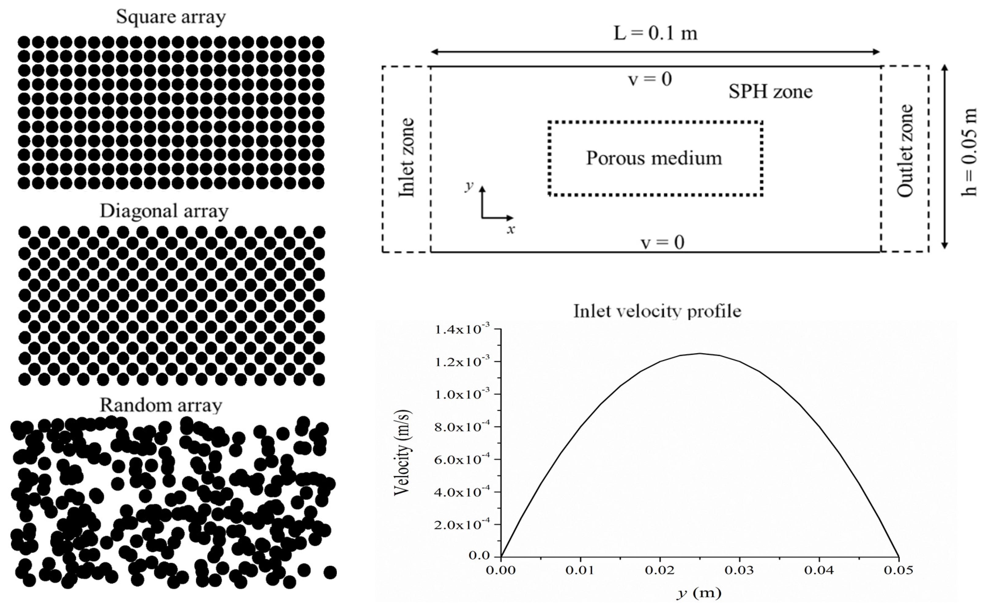
3. Model Problem and Boundary Conditions

The effects of a porous substrate on the incompressible, laminar flow of water in a rectangular channel of length $L=0.1$ m and width $H=0.05$ m are investigated in two-space dimensions. As shown in Figure 1, the channel is subdivided into a clear zone and a rectangular porous layer in its central core of length $L_{pm}=0.05$ m and width $H_{pm}=0.025$ m. The flow is assumed to be isothermal and fully developed so that it enters the channel with a prescribed parabolic velocity profile (see Figure 1). All numerical experiments were conducted using water at room temperature as the working fluid ($\rho =1000$ kg m${}^{-3}$). As displayed in the bottom right picture of Figure 1, the maximum velocity at the inlet is $v_0=1.25\times {10}^{-3}$ m s${}^{-1}$, corresponding to a Reynolds number, Re $=0.0125$. This model problem is the same as that employed by Lai et al. [31] in their lattice Boltzmann calculations with a corrected Ergun equation for high porosity and open-celled substrates. In contrast to Lai et al. [31], here, the simulations were conducted for substrate porosities $\varphi =0.3$, 0.44, 0.55, 0.77 and 0.88. The simulations at the REV scale were performed using the same geometry and parameters as the simulations at the pore scale. In this latter case, three different porous geometries were studied, corresponding to regular non-staggered square, regular staggered square and random arrays of circular grains, as shown in the frames of the left column of Figure 1 for the particular case when $\varphi =0.44$.

No-slip boundary conditions are applied at the walls of the channel ($\mathbf{v}=\mathbf{0}$), using the method of dynamic boundary particles implemented in DualSPHysics [57]. The implementation of this boundary condition parallels that described by Alvarado-Rodríguez et al. [62] for flow in rigid pipes of circular cross-section. Non-reflective outflow boundary conditions are implemented at the exit of the channel [63]. This method allows for anisotropic wave propagation across the outlet plane, where the velocity vector of particles in the outflow zone is evolved using the outgoing wave equation

$$\frac{\partial \mathbf{v}}{\partial t}+v_x\frac{\partial \mathbf{v}}{\partial x}-\nu \frac{{\partial }^2\mathbf{v}}{\partial y^2}=\mathbf{0},$$

(22)

where $\mathbf{v}=(v_x,v_y)$. Here, the $v_x$-velocity component corresponds to the mainstream velocity along the channel. For an outflow particle, say o, the above equation admits the numerically stable SPH representation

$$\frac{\partial {\mathbf{v}}_o}{\partial t}=-v_{x,o}\sum _{b=1}^n\frac{m_b}{{\overline{\rho }}_{ob}}\left({\mathbf{v}}_b-{\mathbf{v}}_o\right)\frac{\partial W_{ab}}{\partial x_o}+2\nu \sum _{b=1}^n\frac{m_b}{{\rho }_b}\frac{y_{ob}\left({\mathbf{v}}_b-{\mathbf{v}}_o\right)}{|{\mathbf{x}}_{ob}{|}^2+{ϵ}^2}\frac{\partial W_{ab}}{\partial y_o},$$

(23)

where ${\mathbf{x}}_{ob}={\mathbf{x}}_o-{\mathbf{x}}_b$, $y_{ob}=y_o-y_b$ and ${\overline{\rho }}_{ob}=({\rho }_o+{\rho }_b)/2$. According to Equation (23), outflow particles near the outlet plane will have some neighbors pertaining to the fluid domain behind the outlet, thus allowing fluid information to be conveyed into the outflow zone with no noise reflection into the fluid domain. The position of outflow particles is evolved by solving the equation

$$\frac{d{\mathbf{x}}_o}{dt}={\mathbf{v}}_o,$$

(24)

which is then time-integrated simultaneously with Equation (23) using the same symplectic integrator employed for the hydrodynamics.

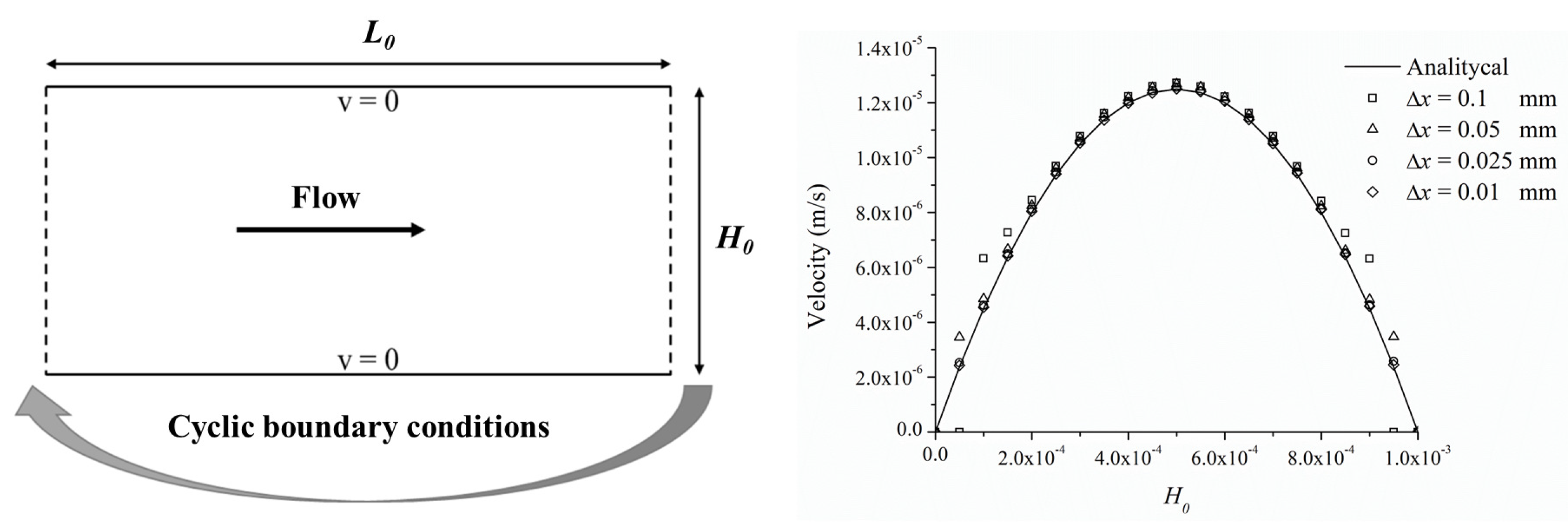
4. Validation and Convergence Testing

The Dualphysics code has been thoroughly validated against experimental data in pipe flow simulations using different geometries [62,64] and for many other benchmark test cases [57]. As a validation test, we further consider unsteady plane Poiseuille flow in a rectangular channel, while the convergence test is performed by comparing the REV-scale mainstream velocity profile at the outlet plane of the rectangular channel with that obtained at the pore scale for a uniform, non-staggered array of grains for $\varphi =0.3$ at varying spatial resolution.

As shown in Figure 2, the channel consists of two infinite, parallel plates, and the $(x,y)$-plane is chosen to represent the flow with the positive x-axis as the flow direction. The plates are located at distances $H_0/2=\pm 0.0005$ m from the center ($y=0$) of the coordinate system. For this problem, the y-components of the velocity and pressure gradient vanish identically so that the x-component of the velocity depends only on y and time. The particles are initially at rest and moved through the channel by applying a body force, $F_b$, due to the hydrostatic pressure gradient $\Delta p/L_0$

$$F_b=\frac{1}{\rho }\left(\frac{\Delta p}{L_0}\right)=-\frac{8\nu v_0}{H_0^2},$$

(25)

where $L_0=0.005$ m is the length of the channel plates and $v_0$ is the velocity at the vertex of the asymptotic (steady-state) velocity profile

$$v_x\left(y\right)=\frac{F_b}{2\nu }\left(y^2-\frac{H_0^2}{4}\right)=v_0\left(1-\frac{4y^2}{H_0^2}\right).$$

(26)

We choose initial parameters similar to those employed by Morris et al. [65] and Sigalotti et al. [66], i.e., ${\rho }_0=1000$ kg m${}^{-3}$, $v_0=1.25\times {10}^{-5}$ m s${}^{-1}$ and Re $=0.0125$, resulting in a kinematic viscosity $\nu =H_0{v}_0/\mathrm{Re}=1.0\times {10}^{-6}$ m${}^2$ s${}^{-1}$.

Convergence to the analytical solution was assessed by increasing the spatial resolution from $N=550$ to 50,601 SPH fluid particles. For simplicity, the particles are initially arranged in a regular Cartesian mesh, and the simulations are followed until a steady-state solution is achieved. For the above resolutions, the initial interparticle distance varies between 0.1 mm (for $N=550$) and 0.01 mm (for N = 50,601). Inlet and outlet boundary conditions during the calculations were handled by means of a cyclic boundary condition, which is enforced by placing five columns of imaginary particles to the left ($y<0$) and to the right ($y>L_0$) of the fluid domain. The right picture of Figure 2 shows the numerically obtained profiles (symbols) as compared with the analytical solution (solid line) at $t=0.6$ s, when the simulations have reached a steady-state solution. At the maximum resolution tried, the numerical profile (filled dots) closely overlaps the analytical solution with a deviation in terms of a root-mean-square error (RMSE) $\lesssim 5.3\times {10}^{-6}$%. At this resolution, the numerical results show a very good matching with the exact solution.

In order to provide internally coherent flow conditions for the subsequent simulations of flow through a rectangular channel with a partially filled porous layer, a convergence test was carried out by varying the total number of particles, N. Upon increasing the number of particles, the results at the REV scale are compared with those obtained at the pore scale using 8,006,801 SPH particles for the case when the porous layer consists of a uniform, non-staggered array of grains with porosity $\varphi =0.3$. This value is below the range $0.4\le \varphi \le 0.6$ for which the Ergun equation is customarily applied to calculate the flow resistance of packed beds and spherical granular materials [28]. Convergence to the pore-scale solution is measured by varying the number of particles at the REV scale from N = 1,082,952 to N = 8,006,801. The results of the convergence study are reported in Figure 3. As shown in Figure 3a, the mainstream velocity profiles at the REV and pore scale are compared at the exit plane of the rectangular channel at different spatial resolutions from N = 1,082,952 ($\Delta x=0.068$ mm) to N = 8,006,801 ($\Delta x=0.025$ mm), while the same is displayed in Figure 3b for the mainstream velocity profile along the channel in the top clear zone. The deviations between both profiles in terms of the RMSE metric are: ∼$7.42\times {10}^{-5}$ m s${}^{-1}$ (for N = 1,082,952), ∼$4.43\times {10}^{-5}$ m s${}^{-1}$ (for N = 2,003,401), ∼$2.20\times {10}^{-5}$ m s${}^{-1}$ (for N = 4,084,654) and ∼$1.98\times {10}^{-5}$ m s${}^{-1}$ (for N = 8,006,801) in Figure 3a, while in Figure 3b, the RMSEs are: ∼$1.58\times {10}^{-4}$ m s${}^{-1}$ (for N = 1,082,952), ∼$9.93\times {10}^{-5}$ m s${}^{-1}$ (for N = 2,003,401), ∼$4.66\times {10}^{-5}$ m s${}^{-1}$ (for N = 4,084,654) and ∼$1.89\times {10}^{-5}$ m s${}^{-1}$ (for N = 8,006,801). In both cases, the numerical profiles at the REV scale show an asymptotic tendency to globally converge to the highly resolved pore-scale solution as the number of particles is increased. The pore-scale simulations use exactly the same SPH solver and also the same number of SPH particles. In both cases, the actual number of particles (i.e., N = 8,006,801) was chosen based on convergence considerations.

5. Results

The results from the REV-scale simulations are compared with those obtained at the pore-scale approach for the three different grain geometries shown in Figure 1. The comparison here is enforced in terms of the mean velocity profiles at the outlet section of the rectangular channel and the pressure losses across the porous medium.

5.1. Flow Structure and Velocity Profiles

A comparison of the mainstream velocity field across the channel between the pore scale (for the three grain geometries) and the REV scale is shown in Figure 4 for the case when the porosity is $\varphi =0.44$. Similar plots are also seen for the other porosity values. In the four cases, the flow structure looks qualitatively similar in the clear zone and across the porous layer. The flow similarity between the pore and REV scales is not surprising, because the classical Ergun equation is known to work satisfactorily well for intermediate porosity values in the range $0.4\lesssim \varphi \lesssim 0.6$ [28]. However, quantitative differences may still exist. For example, the maximum velocity in the clear zone is somewhat slower at the REV scale $v_{max}=1.4185\times {10}^{-3}$ m s${}^{-1}$ (Figure 4d) compared to the pore-scale simulations $v_{max}=1.4611\times {10}^{-3}$ m s${}^{-1}$, $v_{max}=1.4923\times {10}^{-3}$ m s${}^{-1}$ and $v_{max}=1.44451\times {10}^{-3}$ m s${}^{-1}$ (Figure 4a–c), respectively, where the maximum velocity increases as the geometry of the packed column is changed from a non-staggered to a staggered square to a completely random array of grains.

The resulting velocity profiles at the outlet plane ($x=L=0.1$ m) of the channel are displayed in Figure 5 for the REV- and the three different pore-scale simulations when the porosity is varied from $\varphi =0.44$ to 0.88. In all cases, the velocity profiles exhibit a wave-like form, where the crests correspond to the maximum flow velocity of fluid coming from the clear zones of the channel (dim yellow streams at the right border planes of all frames in Figure 4) and the valley to the minimum velocity of the fluid coming from the central porous layer (center of blue stripes at the right border planes of all frames in Figure 4).

For $\varphi =0.3$, there is little difference between the REV and the pore-scale profiles when the packed columns consist of non-staggered and staggered uniformly distributed grains. However, at such low porosity, the difference between the REV- and the pore-scale profiles are more pronounced around the zones of maximum velocities (crests) when the porous layer consists of randomly distributed grains. At a higher porosity, corresponding to $\varphi =0.44$ and 0.55, the results for the REV-scale and the pore-scale simulations (for all three packed geometries) exhibit very small differences, with the minimum velocities around the valley being slightly overestimated by the REV-scale approach. When the porosity grows to $\varphi =0.77$ the REV-scale profiles differ from the pore-scale ones mostly for the case of randomly packed grains. At even higher porosity values, as is the case for $\varphi =0.88$, the differences between the REV- and the pore-scale simulations become even larger independently of the geometry of the porous layer.

Figure 6 shows the root-mean-square errors (RMSEs) between the REV-scale and the pore-scale velocity profiles of Figure 5. For each porosity value, the distances between the REV-scale profile and the pore-scale results are displayed for all three geometries of the porous layer. In general, the error is seen to increase with the porosity. It is interesting to see that at porosity values of 0.44 and 0.55, the errors between the REV- and the pore-scale results are almost independent of the geometry of the porous layer. However, at higher porosity, the errors depend more strongly on the geometry of the porous layer and become larger for randomly distributed grains. A similar trend was also observed for $\varphi =0.3$.

5.2. Pressure Losses

Figure 7 displays the pressure losses along the rectangular channel in the clear zones (top and bottom) and center of the porous layer at different porosity values. A comparison between the REV-scale (blue curves) and the pore-scale simulations (black curves) for the case when the grains are distributed in a non-staggered regular array is presented. The results of the REV-scale calculation closely follow those predicted by the pore-scale simulation when $\varphi =0.44$ and 0.55, while the distance between both models progressively increases at higher porosity values. However, the RMSEs between the REV- and the pore-scale results remain sufficiently small even in the worst case when $\varphi =0.88$ (see Figure 7). In this work, we are interested in demonstrating that Ergun model works well for intermediate and relatively high porosity values $0.44<\varphi <0.88$. Moreover, the trends of the pressure along the channel were found to be very similar to those displayed at higher porosities, although the distance between the REV scale and any of the pore-scale geometries reported was a bit longer at $\varphi =0.3$.

An inspection of Figure 7 shows that the flow through the porous layer experiences mean pressure drops of ≈$8.3\times {10}^{-3}$ Pa for $\varphi =0.44$, ≈$8.8\times {10}^{-3}$ Pa for $\varphi =0.55$, ≈$6.7\times {10}^{-3}$ Pa for $\varphi =0.77$ and ≈$6.7\times {10}^{-3}$ Pa for $\varphi =0.88$ at the pore scale. The pressure drop increases as the porosity decreases. This result is consistent with what is expected if the properties of the fluid, such as surface tension, contact angle and density, remain constant. Moreover, under a greater number of obstacles in the porous layer, the sizes of the porous throats decrease, which produces an increase in the flow velocity there and a corresponding greater variation in the pressure.

The results when the geometry of the porous layer consists of a staggered regular distribution of grains are displayed in Figure 8. It is clear that the details of the pressure losses are sensitive to the geometry of the porous medium. In contrast to Figure 7, in this case, the results at the REV scale do not match the ones at the pore scale for porosity values $\varphi \le 0.77$. In all cases, the REV-scale simulations predict pressure losses greater than the pore-scale calculations through the clear zones and the porous layer. Only when $\varphi =0.88$ do the pressure losses appear to follow similar trends for both models. From Figure 8, it follows that compared to Figure 7, the flow through the porous layer undergoes mean pressure losses of ≈$5.3\times {10}^{-3}$ Pa for $\varphi =0.44$, ≈$5.1\times {10}^{-3}$ Pa for $\varphi =0.55$, ≈$4.4\times {10}^{-3}$ Pa for $\varphi =0.77$ and ≈$6.3\times {10}^{-3}$ Pa for $\varphi =0.88$. Figure 9 shows the pressure drops when the geometry of the porous layer consists of randomly distributed grains. The trends are qualitatively similar to the variations displayed in Figure 8. In no case are the profiles at the REV scale matching those at the pore scale when the grains are randomly distributed, implying that the details of the pressure profiles are sensitive to the geometry of the porous medium. In this case, the pressure drops through the porous layer are ≈$5.9\times {10}^{-3}$ Pa for $\varphi =0.44$, ≈$5.5\times {10}^{-3}$ Pa for $\varphi =0.55$, ≈$4.7\times {10}^{-3}$ Pa for $\varphi =0.77$ and ≈$3.3\times {10}^{-3}$ Pa for $\varphi =0.88$. In this case, a clear tendency exists for the pressure drop to increase for decreasing porosity. For comparison, the mean pressure losses at the REV scale (blue curves in Figure 7, Figure 8 and Figure 9) are: $\approx 8.6\times {10}^{-3}$ Pa for $\varphi =0.44$, ≈$8.4\times {10}^{-3}$ Pa for $\varphi =0.55$, ≈$8.3\times {10}^{-3}$ Pa for $\varphi =0.77$ and ≈$8.3\times {10}^{-3}$ Pa for $\varphi =0.88$. Evidently, these figures show that the mean pressure losses across the porous layer are overestimated at the REV scale, which predict larger pressure drops than the pore-scale simulations.

However, as depicted in Figure 10a–c, the RMSEs between the REV- and the pore-scale pressure profiles remain sufficiently small independently of the geometry of the porous layer. However, the actual distance between the REV- and the pore-scale results increases at higher porosity values. For the case of a uniform non-staggered array of grains, the smallest RMSEs between the REV and pore scales occur for $\varphi =0.44$ and 0.55. At higher porosity ($\varphi =0.77$ and 0.88), the RMSEs increase. However, they always remain $\lesssim 2.5\times {10}^{-3}$ Pa (Figure 10a). For a staggered array of grains (Figure 10b), the errors follow a different trend compared to the non-staggered case. In this case, the errors always remain $\lesssim 2.8\times {10}^{-3}$ Pa, and the data appear to be more scattered. A similar trend is also observed for the random array of grains (Figure 10c), where the RMSes are greater at high porosity values ($\varphi =0.77$ and 0.88).

The velocity profiles in Figure 5 follow similar trends to those displayed by Lai et al. [31] for the case of high porosity values $\varphi \ge 0.90$. They proposed to extend the application of Ergun Equation (6) to porous media with a higher porosity and open-celled structure by simply multiplying it by a correction factor as a function of the porosity and specific surface area of the porous medium (see Equations (31) and (32)). However, when applying this correction to the case with $\varphi =0.88$, the results did not change from the $\varphi =0.88$ profiles in Figure 5. In addition, the pressure profiles in Figure 7, Figure 8 and Figure 9 for the REV scale remained essentially the same. In this work, the REV- and pore-scale simulations were carried out using different devices. Therefore, we are not able to provide information about the computational time between both scales. In order to provide a comparison between the performance of both models, the simulations must be carried out using the same device.

6. Conclusions

In this work, the Ergun resistance force term was implemented in the momentum equation using the method of Smoothed Particle Hydrodynamics (SPH). In particular, the open-source DualSPHysics software was employed to study the flow field across a rectangular channel partially filled with a porous layer at different porosity values between 0.44 and 0.88. The flow field, which was modeled at the Representative Elementary Volume (REV) scale, was compared with similar calculations at the pore scale using three different distributions of granular solids to construct the porous medium, namely a regular non-staggered array of grains, a regular staggered array of grains and a randomly distributed array of grains. The comparison between the simulations at the REV and pore scale was made in terms of the mainstream velocity at the outlet of the rectangular channel and the head losses across both the clear and porous zones of the channel.

The main conclusions can be summarized as follows:

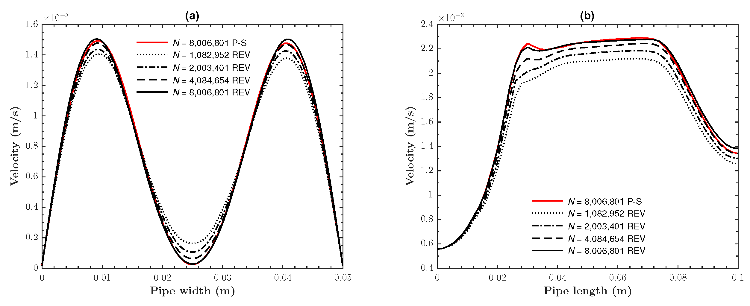
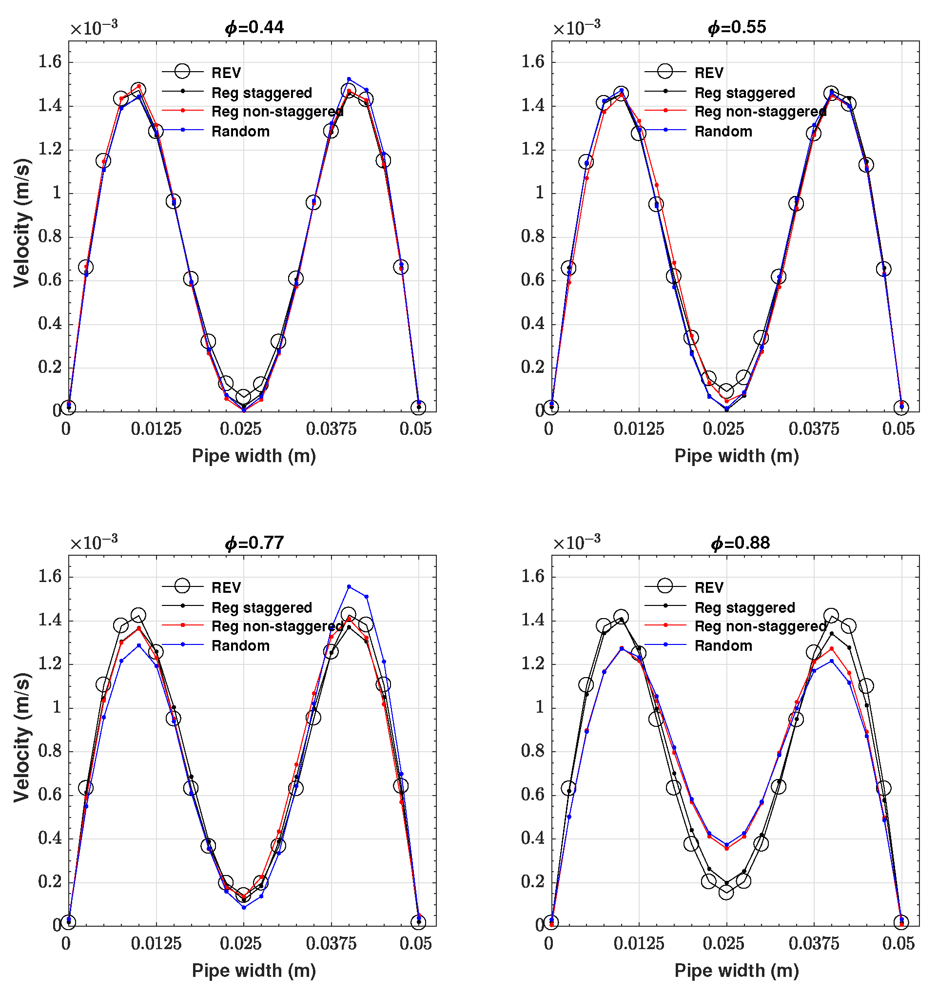
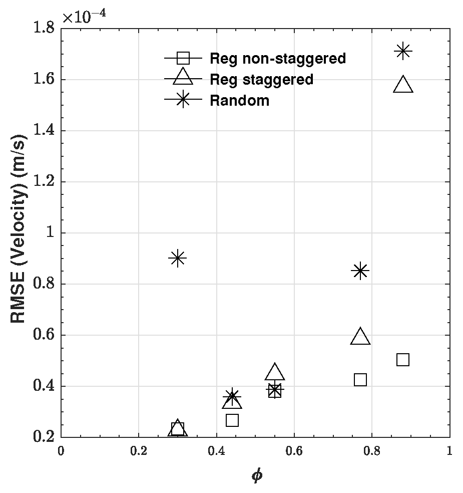
• The results show that the minimum differences in the flow structure and mainstream velocity profiles at the outlet of the rectangular channel between the REV- and the pore-scale simulations always occur at intermediate values of the porosity between 0.44 and 0.55.
• The distance between the REV- and the pore-scale velocity profiles at intermediate porosity as measured in terms of the root-mean-square error (RMSE) is almost independent of the geometry of the porous layer. At higher porosity, the RMSEs grow and depend more strongly on the geometry of the porous medium. However, they always remain at a very low level (i.e., $\lesssim 0.018$%).
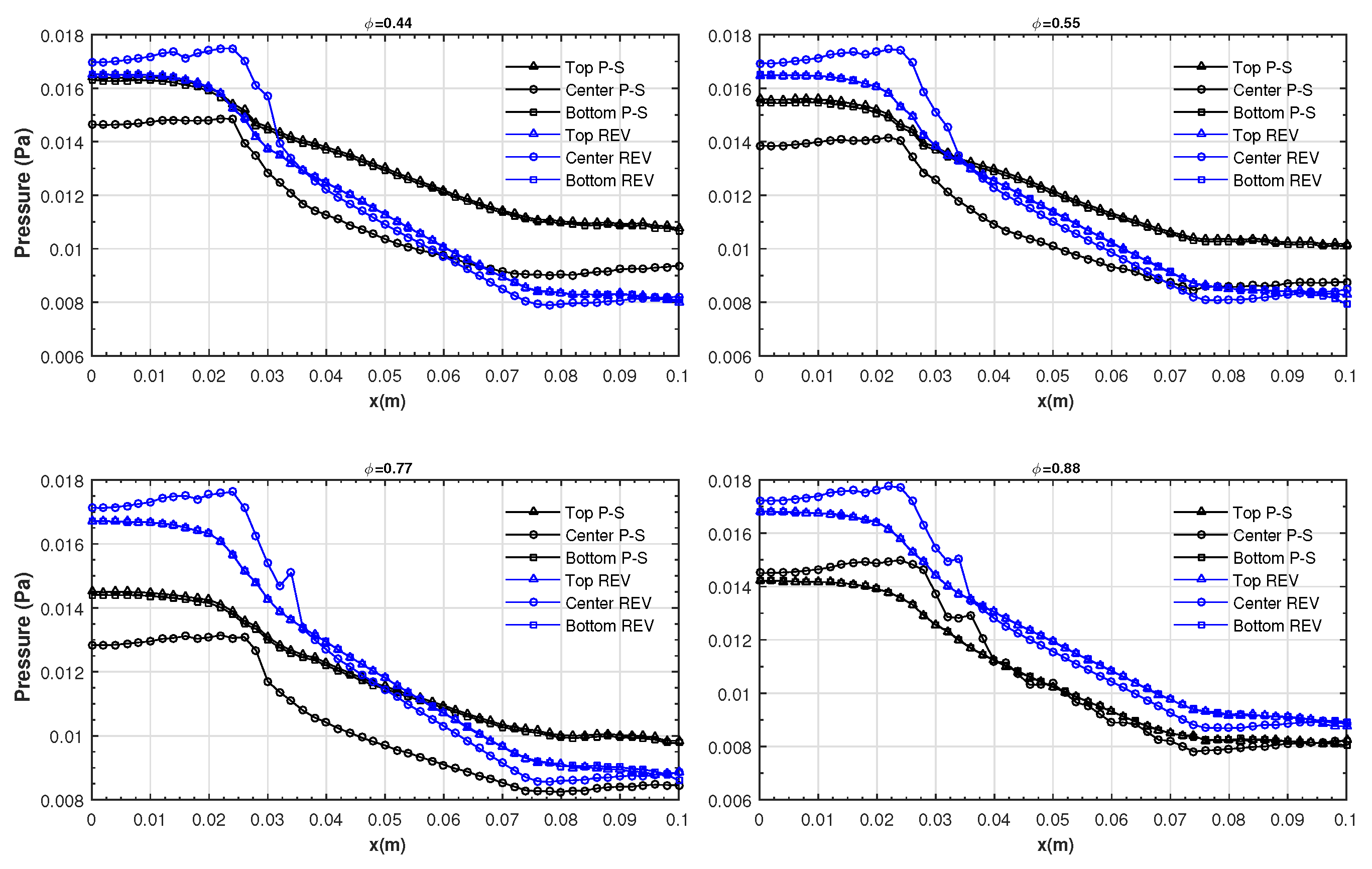
• The pressure losses at the REV scale reproduce those predicted at the pore scale when the grains are uniformly distributed in a non-staggered array with sufficiently good accuracy at intermediate values of the porosity (i.e., $\varphi =0.44$ and 0.55). At higher porosity, the trends of the pressure losses at the REV and pore scale are similar. In general, the distance between the profiles at the REV and pore scale increases with the porosity. However, this distance as measured in terms of the RMSE remains sufficiently small.
• The trends of the pressure losses at the REV and pore scale are affected by the geometry of the porous layer (i.e., by the grain distribution in the packed bed). The discrepancy grows for higher porosity values when the grains are randomly distributed.
• The magnitude of the pressure variations is also affected by the porosity and geometry of the porous medium. In general, the REV-scale simulations predict larger pressure losses compared to any of the pore-scale calculations.

In spite of the fact that no information is provided about the internal structure of the porous medium at the REV scale, the direct comparison with the pore-scale results in terms of the velocity field and outlet velocity profiles revealed a fairly good agreement between both scales, especially at intermediate porosity values. These results confirm that the SPH method is able to accurately describe the flow dynamics through small porous media at the REV scale. This aspect of the results becomes significantly important in larger media where the high computational load associated with such scenarios, such as, for example, in oil reservoirs, may represent an obstacle. On the other hand, the fairly good matching between the REV- and pore-scale results at relatively high porosity values makes the application of the Ergun fixed-bed equation particularly feasible in resistance calculations of porous media with higher porosity and an open-celled structure without the use of empirical corrections.

References

1. Hemond, H.F.; Fechner, E.J. Chemical Fate and Transport in the Environment; Elsevier/Academic Press: Amsterdam, The Netherlands, 2015. [Google Scholar]
2. Katopodes, N.D. Free-Surface Flow. Environmental Fluid Mechanics; Elsevier: Amsterdam, The Netherlands, 2019. [Google Scholar]
3. Xue, L.; Guo, X.; Chen, H. Fluid Flow in Porous Media. Fundamentals and Applications; World Scientific Publishing: Singapore, 2020. [Google Scholar]
4. Liu, M.; Suo, S.; Wu, J.; Gan, Y.; Hanaor, D.A.H.; Chen, C.Q. Tailoring porous media for controllable capillary flow. J. Colloid Interface Sci. 2019, 539, 379–387. [Google Scholar] [CrossRef] [PubMed]
5. Brinkman, H.C. A calculation of the viscous force exerted by a flowing fluid on a dense swarm of particles. Appl. Sci. Res. 1949, 1, 27–34. [Google Scholar] [CrossRef]
6. Liu, H.; Patil, P.R.; Narusawa, U. On Darcy-Brinkman equation: Viscous flow between two parallel plates packed with regular square arrays of cylinders. Entropy 2007, 9, 118–131. [Google Scholar] [CrossRef] [Green Version]
7. Rao, P.R.; Venkataraman, P. Validation of Forchheimer’s law for flow through porous media with converging boundaries. J. Hydraul. Eng. 2000, 126, 63–71. [Google Scholar] [CrossRef]
8. Montillet, A. Flow through a finite packed bed of spheres: A note on the limit of applicability of the Forchheimer-type equation. J. Fluids Eng. 2004, 126, 139–143. [Google Scholar] [CrossRef]
9. Krishnan, S.; Murthy, J.Y.; Garimella, S.V. Direct simulation of transport in open-cell metal foam. J. Heat Transf. 2006, 128, 793–799. [Google Scholar] [CrossRef]
10. Gerbaux, O.; Buyens, F.; Mourzenko, V.V.; Memponteil, A.; Vabre, A.; Thovert, J.F.; Adler, P.M. Transport properties of real metallic foams. J. Colloid Interface Sci. 2010, 342, 155–165. [Google Scholar] [CrossRef]
11. Bai, M.; Chung, J.N. Analytical and numerical prediction of heat transfer and pressure drop in open-cell metal foams. Int. J. Therm. Sci. 2011, 50, 869–880. [Google Scholar] [CrossRef]
12. Mostaghimi, P.; Bijeljic, B.; Blunt, M.J. Simulation of flow and dispersion on pore-space images. SPE J. 2012, 17, 1131–1141. [Google Scholar] [CrossRef] [Green Version]
13. Mostaghimi, P.; Blunt, M.J.; Bijeljic, B. Computations of absolute permeability on micro-CT images. Math. Geosci. 2013, 45, 103–125. [Google Scholar] [CrossRef]
14. Piller, M.; Casagrande, D.; Schena, G.; Santini, M. Pore-scale simulation of laminar flow through porous media. J. Phys. Conf. Ser. 2014, 501, 012010. [Google Scholar] [CrossRef]
15. Mohammadmoradi, P.; Kantzas, A. Pore-scale permeability calculation using CFD and DSMC techniques. J. Pet. Sci. Eng. 2016, 146, 515–525. [Google Scholar] [CrossRef]
16. Niu, Q.; Zhang, C.; Prasad, M. A framework for pore-scale simulation of effective electrical conductivity and permittivity of porous media in the frequency range from 1 mHz to 1GHz. J. Geophys. Res. Solid Earth 2020, 125, e2020JB020515. [Google Scholar] [CrossRef]
17. Bear, J. Dynamics of Fluids in Porous Media; American Elsevier: New York, NY, USA, 1972. [Google Scholar]
18. Succi, S.; Foti, E.; Higuera, F. Three-dimensional floes in complex geometries with the Lattice Boltzmann method. Europhys. Lett. 1989, 10, 433–438. [Google Scholar] [CrossRef]
19. Guo, Z.; Zhao, T.S. Lattice Boltzmann model for incompressible flows through porous media. Phys. Rev. E 2002, 66, 036304. [Google Scholar] [CrossRef]
20. Seta, T.; Takegoshi, E.; Kitano, K.; Okui, K. Thermal Lattice Boltzmann model for incompressible flows through porous media. J. Therm. Sci. Technol. 2006, 1, 90–100. [Google Scholar] [CrossRef] [Green Version]
21. Sukop, M.C.; Huang, H.; Lin, C.L.; Deo, M.D.; Oh, K.; Miller, J.D. Distribution of multiphase fluids in porous media: Comparison between lattice Boltzmann modeling and micro-X-ray tomography. Phys. Rev. E 2008, 77, 026710. [Google Scholar] [CrossRef]
22. Zarghami, A.; di Francesco, S.; Biscarini, C. Porous substrate effects on thermal flows through a REV-scale finite volume lattice Boltzmann model. Int. J. Mod. Phys. C 2014, 25, 1350086. [Google Scholar] [CrossRef]
23. Koekemoer, A.; Luckos, A. Effect of material type and particle size distribution on pressure drop in packed beds of large particles: Extending the Ergun equation. Fuel 2015, 158, 232–238. [Google Scholar] [CrossRef]
24. He, Y.L.; Liu, Q.; Li, Q.; Tao, W.Q. Lattice Boltzmann methods for single-phase and solid-liquid phase-change heat transfer in porous media: A review. Int. J. Heat Mass Transf. 2019, 129, 160–197. [Google Scholar] [CrossRef] [Green Version]
25. Ashorynejad, H.R.; Zarghami, A. Magnetohydrodynamics flow and heat transfer of Cu-water nanofluid through a partially porous wavy channel. Int. J. Heat Mass Transf. 2018, 119, 247–258. [Google Scholar] [CrossRef]
26. Vijaybabu, T.R.; Dhinakaran, S. MHD natural convection around a permeable triangular cylinder inside a square enclosure filled with Al2O3–H2O nanofluid: An LBM study. Int. J. Mech. Sci. 2019, 153-154, 500–516. [Google Scholar] [CrossRef]
27. Ergun, S. Fluid flow through packed columns. Chem. Eng. Prog. 1952, 48, 89–94. [Google Scholar]
28. Zhao, C.Y. Review on thermal transport in high porosity cellular metal foams with open cells. Int. J. Heat Mass Transf. 2012, 55, 3618–3632. [Google Scholar] [CrossRef]
29. du Plessis, J.P.; Woudberg, S. Pore-scale derivation of the Ergun equation to enhance its adaptability and generalization. Chem. Eng. Prog. 2008, 63, 2576–2586. [Google Scholar] [CrossRef]
30. Bazmi, M.; Hashemabadi, S.H.; Bayat, M. Modification of Ergun equation for application in trickle bed reactors randomly packed with trilobe particles using computational fluid dynamics technique. Korean J. Chem. Eng. 2011, 28, 1340–1346. [Google Scholar] [CrossRef]
31. Lai, T.; Liu, X.; Xue, S.; Xu, J. Extension of Ergun equation for the calculation of the flow resistance in porous media with higher porosity and open-celled structure. Appl. Therm. Eng. 2020, 173, 115262. [Google Scholar] [CrossRef]
32. Pang, M.; Zhang, T.; Meng, Y.; Ling, Z. Experimental study on the permeability of crushed coal medium based on the Ergun equation. Sci. Rep. 2021, 11, 23030. [Google Scholar] [CrossRef]
33. Li, Q.; Tang, R.; Wang, S.; Zou, Z. A coupled LES-LBM-IMB-DEM modeling for evaluating pressure drop of a heterogeneous alternating-layer packed bed. Chem. Eng. J. 2022, 433, 133529. [Google Scholar] [CrossRef]
34. Li, Q.; Guo, S.; Wang, S.; Zou, Z. CFD-DEM investigation on pressure drops of heterogeneous alternative-layer particle beds for low-carbon operating blast furnaces. Metals 2022, 12, 1507. [Google Scholar] [CrossRef]
35. Lucy, L.B. A numerical approach to the testing of the fission hypothesis. Astron. J. 1977, 82, 1013–1024. [Google Scholar] [CrossRef]
36. Gingold, R.A.; Monaghan, J.J. Smoothed particle hydrodynamics: Theory and application to non-spherical stars. Mon. Not. R. Astron. Soc. 1977, 181, 375–389. [Google Scholar] [CrossRef]
37. Monaghan, J.J. Smoothed particle hydrodynamics. Rep. Prog. Phys. 2005, 68, 1703–1759. [Google Scholar] [CrossRef] [Green Version]
38. Liu, M.B.; Liu, G.R. Smoothed particle hydrodynamics (SPH): An overview and recent developments. Arch. Comput. Methods Eng. 2010, 17, 25–76. [Google Scholar] [CrossRef] [Green Version]
39. Liu, G.R.; Liu, M.B. Smoothed Particle Hydrodynamics: A Meshfree Particle Method; World Scientific: Singapore, 2003. [Google Scholar]
40. Morris, J.P.; Zhu, Y.; Fox, P.J. Parallel simulations of pore-scale flow through porous media. Comput. Geotech. 1999, 25, 227–246. [Google Scholar] [CrossRef]
41. Zhu, Y.; Fox, P.J. Smoothed particle hydrodynamics model for diffusion through porous media. Transp. Porous Media 2001, 43, 441–471. [Google Scholar] [CrossRef]
42. Jiang, F.; Oliveira, M.S.A.; Sousa, A.C.M. Mesoscale SPH modeling of fluid flow in isotropic porous media. Comput. Phys. Commun. 2007, 176, 471–480. [Google Scholar] [CrossRef]
43. Tartakovsky, A.M.; Ward, A.L.; Meakin, P. Pore-scale simulations of drainage of heterogeneous and anisotropic porous media. Phys. Fluids 2007, 19, 103301. [Google Scholar] [CrossRef]
44. Tartakovsky, A.M.; Trask, N.; Pan, K.; Jones, B.; Pan, W.; Williams, J.R. Smoothed particle hydrodynamics and its applications for multiphase flow and reactive transport in porous media. Comput. Geosci. 2016, 20, 807–834. [Google Scholar] [CrossRef] [Green Version]
45. Kunz, P.; Zarikos, I.M.; Karadimitriou, N.K.; Huber, M.; Nieken, U.; Hassanizadeh, S.M. Study of multi-phase flow in porous media: Comparison of SPH simulations with micro-model experiments. Transp. Porous Media 2016, 114, 581–600. [Google Scholar] [CrossRef] [Green Version]
46. Kashani, M.N.; Elekaei, H.; Zivkovic, V.; Zhang, H.; Biggs, M.J. Explicit numerical simulation-based study of the hydrodynamics of micro-packed beds. Chem. Eng. Sci. 2016, 145, 71–79. [Google Scholar] [CrossRef] [Green Version]
47. Peng, C.; Xu, G.; Wu, W.; Yu, H.; Wang, C. Multiphase SPH modeling of free surface flow in porous media with variable porosity. Comput. Geotech. 2017, 81, 239–248. [Google Scholar] [CrossRef]
48. Lenaerts, T.; Adams, B.; Dutré, P. Porous Flow in Particle-Based Fluid Simulations. ACM Trans. Graph. 2008, 27, 1–8. [Google Scholar] [CrossRef]
49. Bui, H.H.; Nguyen, G.D. A coupled fluid-solid SPH approach to modelling flow through deformable porous media. Int. J. Solids Struct. 2017, 125, 244–264. [Google Scholar] [CrossRef]
50. Shigorina, E.; Rüdiger, F.; Tartakovsky, A.M.; Sauter, M.; Kordilla, J. Multiscale Smoothed Particle Hydrodynamics Model Development for Simulating Preferential Flow Dynamics in Fractured Porous Media. Water Resour. Res. 2021, 57, e2020WR027323. [Google Scholar] [CrossRef]
51. Bui, H.H.; Nguyen, G.D. Smoothed particle hydrodynamics (SPH) and its applications in geomechanics: From solid fracture to granular behaviour and multiphase flows in porous media. Comput. Geotech. 2021, 138, 104315. [Google Scholar] [CrossRef]
52. Nithiarasu, P.; Seetharamu, K.N.; Sundararajan, T. Natural convective heat transfer in a fluid saturated variable porosity medium. Int. J. Heat Mass Transf. 1997, 40, 3955–3967. [Google Scholar] [CrossRef]
53. Nithiarasu, P.; Seetharamu, K.N.; Sundararajan, T. Effect of porosity on natural convective heat transfer in a fluid saturated porous medium. Int. J. Heat Fluid Flow 1998, 19, 56–58. [Google Scholar] [CrossRef]
54. Becker, M.; Teschner, M. Weakly compressible SPH for free surfaces. In Proceedings of the 2007 ACM SIGGRAPH/Europhysics Symposium on Computer Animation, San Diego, CA, USA, 2–4 August 2007; Metaxas, D., Popovic, J., Eds.; pp. 32–58. [Google Scholar]
55. McCabe, W.L. Unit Operations of Chemical Engineering. Chemical Engineering Series, 7th ed.; McGraw-Hill: New York, NY, USA, 2005. [Google Scholar]
56. Rabbani, A.; Jamshidi, S.; Salehi, S. Determination of specific surface of rock grains by 2D imaging. J. Geophys. Res. 2014, 2014, 945387. [Google Scholar] [CrossRef] [Green Version]
57. Domínguez, J.M.; Fourtakas, G.; Altomare, C.; Canelas, R.B.; Tafuni, A.; García-Feal, O.; Martínez-Estévez, I.; Mokos, A.; Vacondio, R.; Crespo, A.J.C.; et al. DualSPHysics: From fluid dynamics to multiphysics problems. Comput. Part. Mech. 2022, 9, 867–895. [Google Scholar] [CrossRef]
58. Colagrossi, A.; Landrini, M. Numerical simulation of interfacial flows by smoothed particle hydrodynamics. J. Comput. Phys. 2003, 191, 448–475. [Google Scholar] [CrossRef]
59. Bonet, J.; Lok, T.S.L. Variational and momentum preservation aspects of smoothed particle hydrodynamics formulations. Comput. Methods Appl. Mech. Eng. 1999, 180, 97–115. [Google Scholar] [CrossRef]
60. Lo, E.Y.M.; Shao, S. Simulation of near-shore solitary wave mechanics by an incompressible SPH method. Appl. Ocean. Res. 2002, 24, 275–286. [Google Scholar] [CrossRef]
61. Dehnen, W.; Aly, H. Improving convergence in smoothed particle hydrodynamics simulations without pairing instability. Mon. Not. R. Astron. Soc. 2012, 425, 1068–1082. [Google Scholar] [CrossRef] [Green Version]
62. Alvarado-Rodríguez, C.E.; Sigalotti, L.D.G.; Klapp, J.; Fierro-Santillán, C.R.; Aragón, F.; Uribe-Ramírez, A.R. Smoothed particle hydrodynamics simulations of turbulent flow in curved pipes with different geometries: A comparison with experiments. J. Fluids Eng. 2021, 143, 091503. [Google Scholar] [CrossRef]
63. Alvarado-Rodríguez, C.E.; Klapp, J.; Sigalotti, L.D.G.; Domínguez, J.M.; de la Cruz Sánchez, E. Nonreflecting outlet boundary conditions for incompressible flows using SPH. Comput. Fluids 2017, 159, 177–188. [Google Scholar] [CrossRef] [Green Version]
64. Sigalotti, L.D.G.; Alvarado-Rodríguez, C.E.; Klapp, J.; Cela, J.M. Smoothed particle hydrodynamics simulations of water flow in a 90° pipe bend. Water 2021, 13, 1081. [Google Scholar] [CrossRef]
65. Morris, J.P.; Fox, P.J.; Zhu, Y. Modeling low Reynolds number incompressible flows using SPH. J. Comput. Phys. 1997, 136, 214–226. [Google Scholar] [CrossRef]
66. Sigalotti, L.D.G.; Klapp, J.; Sira, E.; Meleán, Y.; Hasmy, A. SPH simulations of time-dependent Poiseuille flow at low Reynolds numbers. J. Comput. Phys. 2003, 191, 622–638. [Google Scholar] [CrossRef]
Figure 1. Geometries of the porous media employed in the pore-scale simulations for the case when ϕ = 0.44 (left column of frames), schematic diagram of the problem at REV scale (top right) and steady-state inlet velocity profile used in all simulations (bottom right).
Water 15 02358 g001
Figure 2. Schematic diagram showing the geometry for the plane Poiseuille flow test problem (left picture) and numerical steady-state velocity profiles at different spatial resolutions (symbols) as compared to the analytical solution (solid line).
Water 15 02358 g002
Figure 3. (a) REV-scale velocity profiles at the exit plane of the rectangular channel at different spatial resolutions as compared with the pore-scale solution with N = 8 , 006 , 801 SPH particles (red curve). (b) The same for the mainstream velocity profile along the channel in the top clear zone.
Water 15 02358 g003
Figure 4. Mainstream fluid velocity across the channel obtained from the pore-scale simulations when the interposed porous layer consists of (a) a non-staggered square, (b) a staggered square and (c) a random array of circular grains as compared to (d) the REV-scale simulation for ϕ = 0.44 .
Water 15 02358 g004
Figure 5. Mainstream velocity profiles at the outlet plane of the channel for the REV- and pore-scale simulations at different porosity values between ϕ = 0.44 and 0.88. The profiles obtained at the pore scale for the three different geometries of the porous layer are compared with the REV-scale results.
Water 15 02358 g005
Figure 6. Root-mean-square error (RMSE) as a function of the porosity for the velocity profiles at the outlet plane of the channel (see Figure 5). The symbols identify the geometry of the porous layer.
Water 15 02358 g006
Figure 7. Pressure losses predicted by the REV-scale simulation (blue curves) as compared with the pore-scale calculation when the porous layer consists of grains distributed in a regular non-staggered way (black curves). The results are displayed for the top and bottom clear zones and for the center of the porous layer.
Water 15 02358 g007
Figure 8. Pressure losses predicted by the REV-scale simulation (blue curves) as compared with the porous-scale calculation when the porous layer consists of grains distributed in a regular staggered way (black curves). The results are displayed for the top and bottom clear zones and for the center of the porous layer.
Water 15 02358 g008
Figure 9. Pressure losses predicted by the REV-scale simulation (blue curves) as compared with the porous-scale calculation when the porous layer consists of randomly distributed grains (black curves). The results are displayed for the top and bottom clear zones and for the center of the porous layer.
Water 15 02358 g009
Figure 10. Root-mean-square errors (RMSEs) as functions of the porosity for the pressure losses between the REV- and pore-scale results of (a) Figure 7 for a non-staggered regular array of grains, (b) Figure 8 for a staggered regular array of grains and (c) Figure 9 for a randomly distributed array of grains.
Water 15 02358 g010
Disclaimer/Publisher’s Note: The statements, opinions and data contained in all publications are solely those of the individual author(s) and contributor(s) and not of MDPI and/or the editor(s). MDPI and/or the editor(s) disclaim responsibility for any injury to people or property resulting from any ideas, methods, instructions or products referred to in the content.