Forecasting of Standardized Precipitation Index Using Hybrid Models: A Case Study of Cape Town, South Africa

Abstract

Droughts have negative impacts on agricultural productivity and economic growth. Effective monitoring and accurate forecasting of drought occurrences and trends are crucial for minimizing drought losses and mitigating their spatial and temporal effects. In this study, trend dynamics in monthly total rainfall time series measured at Cape Town International Airport were analyzed using the Mann–Kendall (MK) test, Modified Mann–Kendall (MMK) test and innovative trend analysis (ITA). Additionally, we utilized a hybrid prediction method that combined the model with the complementary ensemble empirical mode decomposition with adaptive noise (CEEMDAN) technique, the autoregressive integrated moving average (ARIMA) model, and the long short-term memory (LSTM) network (i.e., CEEMDAN-ARIMA-LSTM) to forecast SPI values of 6-, 9-, and 12-months using rainfall data between 1995 and 2020 from Cape Town International Airport meteorological rainfall stations. In terms of trend analysis of the monthly total rainfall, the MK and MMK tests detected a significant decreasing trend with negative z-scores of −3.7541 and −4.0773, respectively. The ITA also indicated a significant downward trend of total monthly rainfall, especially for values between 10 and 110 mm/month. The SPI forecasting results show that the hybrid model (CEEMDAN-ARIMA-LSTM) had the highest prediction accuracy of the models at all SPI timescales. The Root Mean Square Error (RMSE) values of the CEEMDAN-ARIMA-LSTM hybrid model are 0.121, 0.044, and 0.042 for SPI-6, SPI-9, and SPI-12, respectively. The directional symmetry for this hybrid model is 0.950, 0.917, and 0.950, for SPI-6, SPI-9, and SPI-12, respectively. This indicates that this is the most suitable model for forecasting long-term drought conditions in Cape Town. Additionally, models that use a decomposition step and those that are built by combining independent models seem to produce improved SPI prediction accuracy.

1. Introduction

Drought is a gradual and pernicious natural catastrophic event with global socioeconomic and environmental consequences. This is a highly perilous climate-related catastrophe that has a substantial effect on both the environment and human existence [1]. Droughts have a profound effect on municipal water supplies, which is one of their most important effects. These supplies refer to the purified water distributed to households and businesses, which is crucial for human consumption, cleanliness, and numerous critical services on a global scale [2]. Municipal water sources are given priority during drought and water constraint due to their significant sociological and economic relevance. This prioritization entails reallocating available water resources, frequently diverting them away from other sectors, especially agriculture, to ensure the uninterrupted supply of water to urban areas and their residents [3]. During extremely severe drought circumstances, the water sources that urban water systems depend on can be exhausted, leading to a scarcity of municipal water for consumers.

In 2018, Cape Town and other parts of the country faced acute water shortages as a result of drought. These occurrences and growing concerns about water scarcity in urban areas are the result of several factors, including rising demand for water due to population growth, unpredictable weather patterns, the effects of climate change, and, in some cases, insufficient planning and management of water infrastructure [4,5]. In addition, the exploitation of surface water and groundwater resources, which have historically supplied water for human sustenance and agriculture, has reached unsustainable levels in several countries, resulting in negative environmental consequences [6]. The excessive use of these natural water resources has led to the contamination of certain water bodies, such as the salinization of over-exploited aquifers or the inability to dilute and assimilate wastewater discharges, rendering the water supplies unsuitable for human consumption [7]. To maintain a secure and stable water supply in the present and the future, it is essential to recognize that the development of resilient water systems is an imperative necessity [8]. In disaster management, the application of time series forecasting methodologies can serve as an early warning system.

The main aim of drought risk analysis is to improve drought management and forecasting techniques. It focuses on various aspects of droughts, such as their size, duration, intensity, and spatial extent [9]. Droughts develop slowly, and their consequences become apparent over a long period of time. To monitor and predict droughts, various drought indices are used to measure the deviation of meteorological variables, such as precipitation, from their long-term averages [10]. In general, drought monitoring relies on several indices, including the Palmer Drought Severity Index (PDSI) [11], Effective Drought Index (EDI) [12], Reconnaissance Drought Index (RDI) [13], Standardized Precipitation Evapotranspiration Index (SPEI) [14], Weighted Anomaly Standardized Precipitation Index (WASP) [15], and Standardized Drought Indices (SDIs) [16]. A comprehensive list of these indices and their descriptions can be found in Zargar et al. [17]. However, the most widely used method for drought monitoring using drought indices is the Standardized Precipitation Index (SPI) [18], primarily because it only uses one parameter (precipitation).

The SPI, developed by McKee et al. [18], is widely used as a global drought monitoring tool following the Lincoln Drought Declaration of the World Meteorological Organization [19,20]. What sets the SPI apart from other indices is its simplicity, as it relies solely on precipitation data. As a result, it is invaluable for conducting drought risk analysis and estimations in areas where data are limited and other parameters such as stream flow, evapotranspiration, and soil moisture information may be unavailable [21]. The SPI is applicable across different time periods and geographical areas, and it can be computed for various temporal scales [22]. As a result, it facilitates the assessment of drought duration, magnitude, and severity, while also categorizing droughts into hydrological, agricultural, or environmental types. The SPI’s utilization of a probabilistic approach has solidified its significance in drought analysis, making it a widely adopted tool in many global regions. Hence, accurate estimation of the SPI is crucial for comprehensive drought analysis.

To date, a multitude of research papers have been published on the estimation of drought indices using data-driven techniques [23,24,25,26,27,28]. The significance of addressing drought-related issues has increased as time series analysis continues to advance. Prediction of drought requires the management of complex, often nonstationary, nonlinear precipitation data, and SPI time series. Rarely do we encounter simple and stable time series in practice. Consequently, it is of the utmost importance to identify an efficient method for addressing the complexities of nonlinear and nonstationary time series and for making accurate forecasts. In the realm of developing data-based drought forecasting models, linear approaches, such as the utilization of autoregressive integrated moving average (ARIMA) models, have been superseded by nonlinear approaches rooted in Artificial Intelligence models in recent years. Nonetheless, due to the complexities of evaluating time series precision, devising suitable forecasting models remains a formidable challenge [29].

In recent years, numerous models, such as the Autoregressive Integrated Moving Average (ARIMA) model, have been utilized for drought forecasting due to its their adaptability and greater information on time-related changes [30]. However, the ARIMA model has certain limitations that make it unsuitable for forecasting hydrometeorological time series, especially when dealing with nonstationarity and nonlinearities [31]. According to Achite et al. 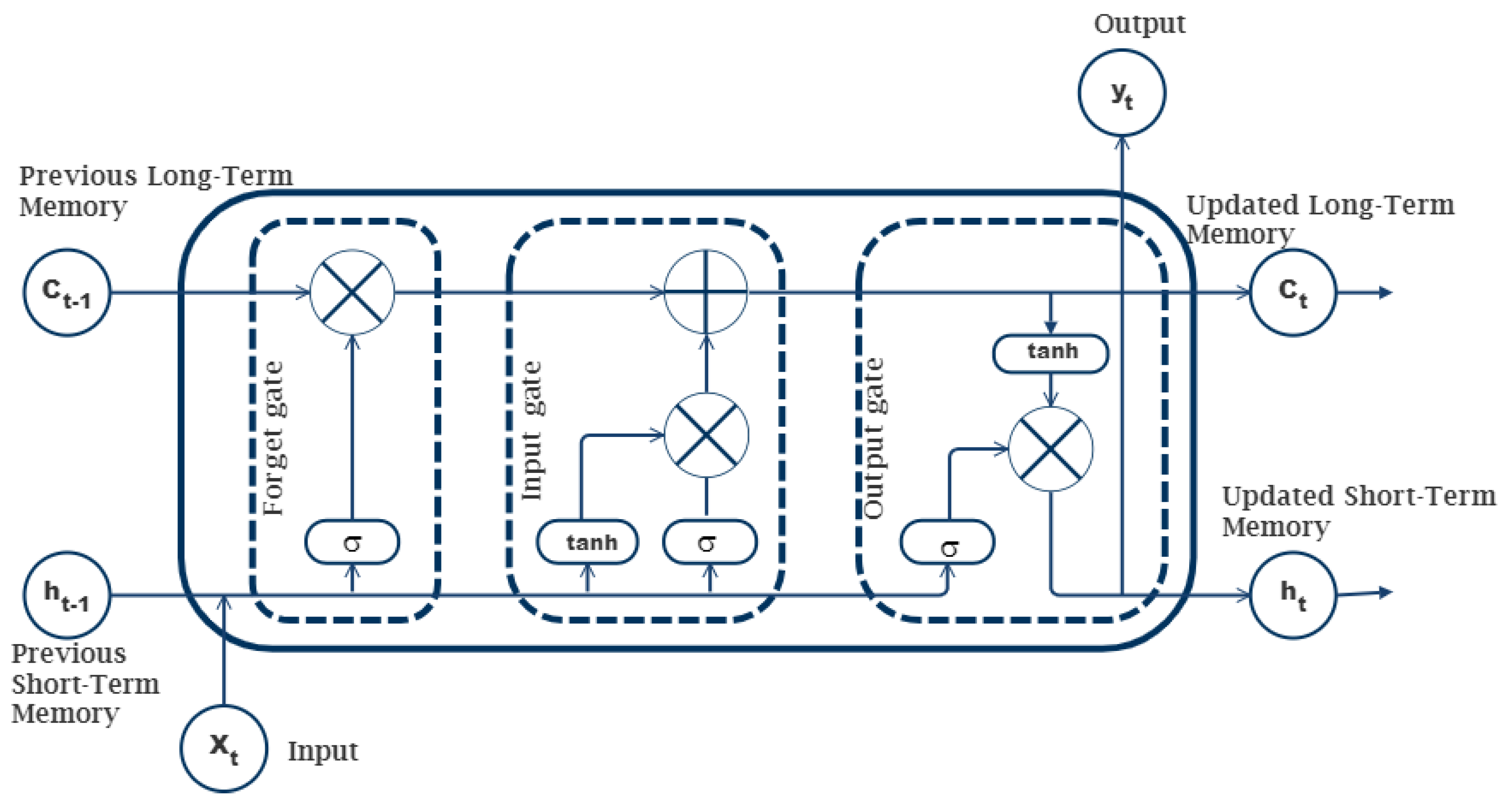[32], machine learning techniques have limited ability to anticipate nonstationary drought time series. As machine learning has evolved, the long short-term memory (LSTM) network has emerged as a solution to resolve long-term dependencies, especially in sequences with extended intervals and delays [33]. The LSTM model has shown promising results when applied to the prediction of drought time series and related domains [34,35,36]. Nonetheless, the inherent complexity of time series frequently results in suboptimal local predictions, thereby diminishing the overall performance of forecasting [37].

To enhance time series prediction accuracy in the face of these complexities, scholars have introduced signal decomposition techniques [38,39,40,41]. Utilizing data pre-processing techniques, such as wavelet transform and decomposition methods, proves to be a highly effective approach in addressing this limitation [42]. A study by Belayneh et al. [43] emphasized the utility of wavelet transform as a valuable tool for data preprocessing, effectively decomposing the original dataset. This is particularly advantageous in predicting nonlinear and nonstationary time series. The wavelet transform enables the extraction of vital information at varying levels of detail, subsequently enhancing the performance of machine learning models. Rezaiy and Shabri [44] utilized a hybrid modelling technique known as wavelet transform and ARIMA (W-ARIMA) in their drought forecasting study conducted in Kabul, Afghanistan. In their study, they utilized the Daubechies function of order 2 with a decomposition level of 3 for the wavelet transform. The integrated W-ARIMA method demonstrated superior performance in comparison to classic ARIMA techniques for SPI-based series in the short, medium, and long-term.

For the processing of nonstationary and nonlinear data with frequency components, the use of decomposition techniques serves as an additional preprocessing method in conjunction with the wavelet transform. In the context of predicting drought, decomposition emerges as a valuable tool when compared to wavelet transformation. Wavelet transform may have limitations due to a lack of sufficient mother wavelet functions or restricted decomposition levels. Signal decomposition efficiently removes certain characteristics from sequences, making them more stable and easier to handle. These methods streamline the initial simplified time series and enhance their predictability. Some of the methods include empirical mode decomposition (EMD), ensemble empirical mode decomposition (EEMD), complementary ensemble empirical mode decomposition (CEEMD), and complementary ensemble empirical mode decomposition with adaptive noise (CEEMDAN). CEEMD addresses both the problem of blending modes in EMD and the issue of residual white noise in EEMD. Furthermore, CEEMDAN is an enhanced iteration of CEEMD that provides enhanced adaptability in handling intricate signals with varying attributes and levels of noise. CEEMDAN is specifically intended to adaptively assess and remove noise from the signal throughout the decomposition process. This is especially advantageous when the input signal is contaminated by noise, as it enhances the integrity of the recovered components. The combination of decomposing techniques and prediction models has demonstrated potential in improving the prediction of drought in time series data [45]. In the study conducted by Libanda and Nkolola [46], it is demonstrated that the hybrid model exhibits greater proficiency in managing the intricacies of drought forecasting through the integration of EMD. This integration effectively addresses the limitations of ARIMA’s exclusively linear and stationary approach. Xu et al. [47] utilized the CEEMD-ARIMA combined model to forecast drought in the Xinjiang Uygur Autonomous Region of China. The model outperformed the standalone ARIMA in terms of prediction accuracy across many timescales. Ding et al. [37] utilized a hybrid model combining CEEMD-LSTM to predict drought in the Xinjiang Uygur Autonomous Region of China using the standardized precipitation index. The hybrid model demonstrated superior performance compared to LSTM.

Drought forecasting, particularly for different lead times, remains a challenging task [48]. In the literature of drought prediction, several methods using the hybrid approach for accurately predicting the SPI have been extensively discussed in recent years [49,50]. These hybrid methods have shown remarkable efficacy in SPI prediction, producing outstanding performance results. Despite these advancements, there is still a need for models that can accurately predict drought indices such as the SPI across diverse climatic conditions and temporal scales. The importance of accurate SPI drought prediction lies in its ability to provide and plays a pivotal role in efficient water resource management, decision-makers, policymakers and climate adaptation. Conventional models like ARIMA frequently encounter challenges in capturing the intricate, nonlinear characteristics of climatic data. While LSTM can address nonstationarity and nonlinearity through functions, optimizing its performance often entails preprocessing the data to unveil inherent patterns. Recent advancements, such as the CEEMDAN technique, hold promise for enhancing predictive accuracy by decomposing time series data into IMFs.

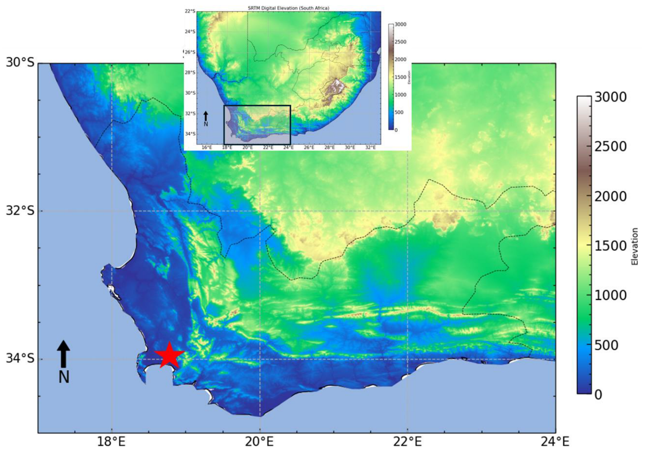
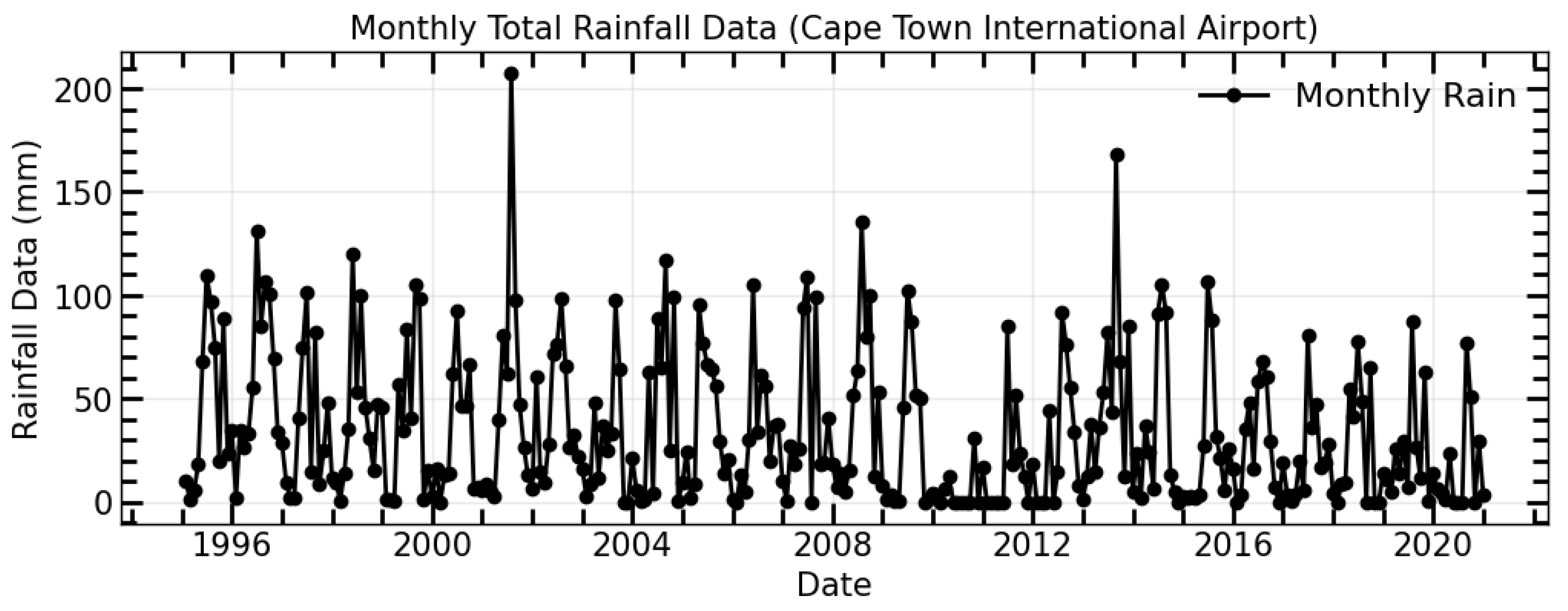
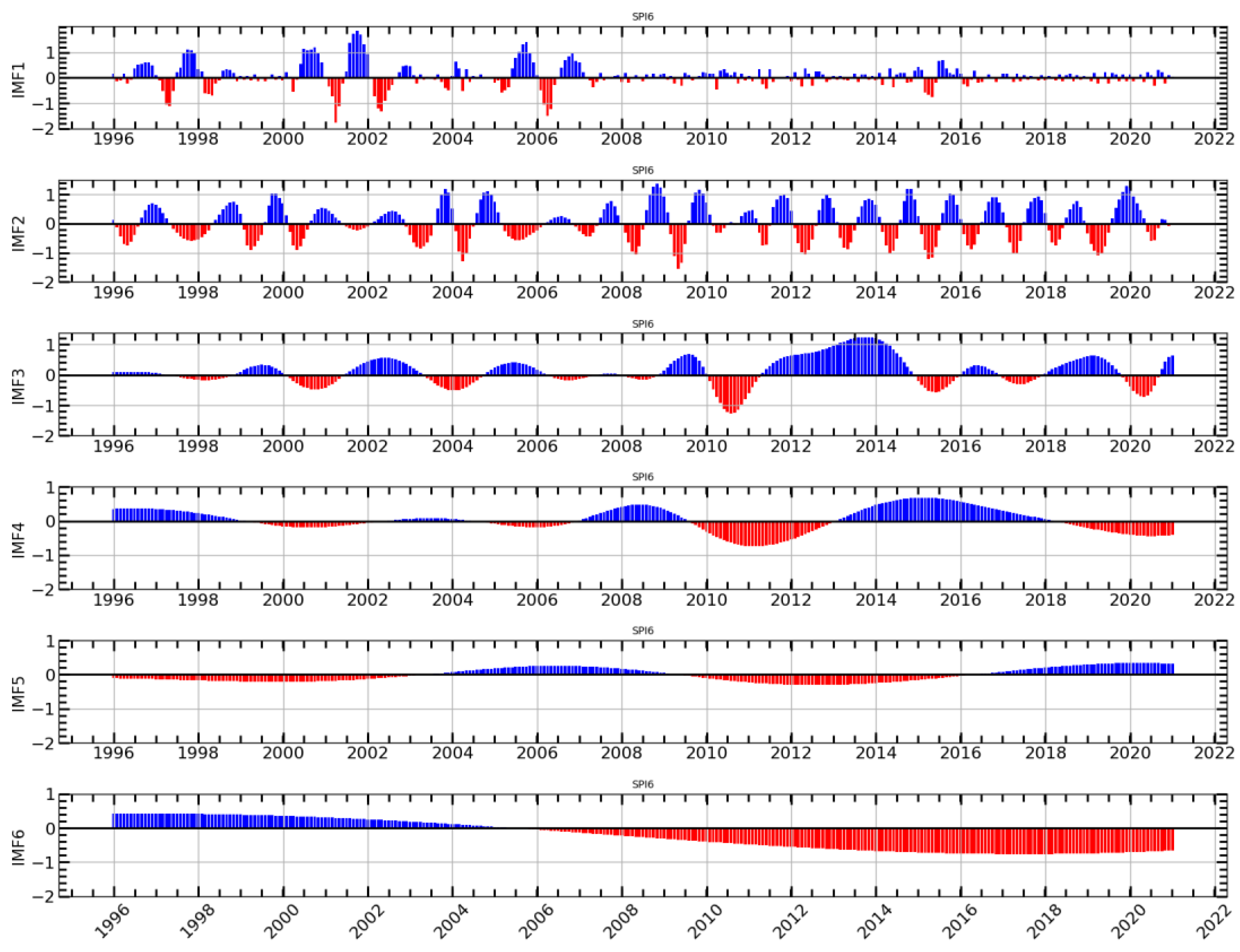
Due to the complexities associated with the nonlinear and nonstationary nature of precipitation data, our objective is to investigate more efficient methods for time series prediction. However, there is a lack of extensive research on the integration of CEEMDAN with ARIMA-LSTM for drought prediction in South Africa. The objective of the study is to enhance the precision of drought prediction by capitalizing on the strengths of these methods in managing intricate time series. Specifically, the study aims to (i) decompose precipitation data using CEEMDAN into five IMFs and one residual component; (ii) predict each IMF and the residual using ARIMA, LSTM, and ARIMA-LSTM; (iii) combine the forecasts of each IMF and residual to obtain the final drought prediction; and (iv) evaluate the accuracy of the proposed method against traditional ARIMA and LSTM models, as well as advanced methodologies used in previous studies. The focus of the study is on Cape Town International Airport in the Western Cape province of South Africa, an area with unique drought dynamics that have not been explored using hybrid methodologies before. By combining CEEMDAN and ARIMA-LSTM, our innovative model not only fills this research gap but also provides a pioneering solution that can significantly improve accuracy in drought forecasting. Through rigorous evaluation against established benchmarks such as ARIMA and LSTM, we aim to demonstrate the superior performance of our hybrid approach, thereby solidifying its significance in advancing the field of drought prediction.

2. Materials and Methods

2.1. Study Area

The data used in the study were measured at Cape Town International Airport (see Figure 1), located in the Western Cape province of South Africa. This figure shows the Shuttle Radar Topography Mission (SRTM) digital elevation profile of the study area, and the rain gauge station (Cape Town International Airport) is indicated by a red star. The exact geographical coordinates are approximately 33.9249° S latitude and 18.4241° E longitude. This coastal city is located on the southwestern coast of South Africa, between the Atlantic Ocean to the west and the Hottentots-Holland Mountains to the east, creating a breathtaking natural environment that includes picturesque coastlines and Table Mountain. The unique geographical location of Cape Town has played a significant role in its history and development, contributing to the city’s breathtaking natural attractiveness.

2.2. Mann–Kendall Test Statistics

Examining potential changes in the characteristics of precipitation events resulting from climate change is of the utmost importance as it has significant implications for soil moisture retention, hazard assessment, and flood management. The assessment of monotonous trends in a time series of geophysical data proves consistently advantageous. The Mann–Kendall (MK) test and modified Mann–Kendall (MMK) test are widely used nonparametric statistical methods, serving as effective tools for evaluating trends in time series data. Mann first introduced this test in 1945 [51], and Kendall later refined it in 1975 [52]. The computation of the test statistic $S$ follows the formula below.

$$S=\sum _{j=1}^{n-1}\sum _{i=j+1}^{n}Sign\left(x_i-x_j\right)$$

(1)

$$Sign\left(x\right)=f\left(x\right)=\left\{\begin{array}{c}1 for x>1\\ 0 for x=1\\ -1, for x<1\end{array}\right.$$

(2)

Let n represent the length of the data. The data values at times $i$ and $j$ are denoted as $x_i$ and $x_j$, respectively. According to Seenu and Jayakumar [53], in the Mann–Kendall test, a positive test statistic, S, suggests an increasing trend, whereas a negative test statistic indicates a decreasing trend. The variance for S is calculated using a specific mathematical formula.

$$Var\left(S\right)={\displaystyle \frac{n\left(n-1\right)\left(2n+5\right)-\sum _{i=1}^p{t}_i\left(t_i-1\right)\left(2t_i+5\right)}{18}}$$

(3)

The variable $t_i$ represents the number of data points in the $j^{th}$ tied group, while $p$ represents the number of the tied group in the time series. The statement indicates that the data in a time series can be compared to each other [54]. The summation procedure in Equation (3) is specifically used for linked groups in the time series. Its purpose is to minimize the impact of individual values within tied groups on the ranking statistics [55]. Assuming random and independent time series, the S statistic follows a normal distribution and can be calculated as the standardized Z statistic as follows:

$$Z=\left\{\begin{array}{c}{\displaystyle \frac{S-1}{Var\left(S\right)}} , S>0\\ 0 , S=0 \\ {\displaystyle \frac{S+1}{Var\left(S\right)}} , S<0\end{array}\right.$$

(4)

The Z variable follows a standard normal distribution with a variance of one and a mean of zero. The value of the S statistic is associated with the Kendall term $\tau$, which is defined as

$$\tau ={\displaystyle \frac{S}{D}}$$

(5)

where

$$D={\left[{\displaystyle \frac{1}{2}}n\left(n-1\right)-{\displaystyle \frac{1}{2}}\sum _{j=1}^p{t}_j\left(t_j-1\right)\right]}^{{\displaystyle \frac{1}{2}}}{\left[{\displaystyle \frac{1}{2}}n\left(n-1\right)\right]}^{{\displaystyle \frac{1}{2}}}$$

(6)

The test statistic Z is utilized to quantify the significance of trends. In fact, the null hypothesis of the MK test assumes the absence of any trend and is tested against the alternative hypothesis, which assumes the presence of a trend at a specific level of significance [56,57]. Another significant outcome of the Mann–Kendall statistics is the Kendall term, which measures the correlation and indicates the strength of the relationship between any two independent variables. For serially correlated data, having a significant lag-1 autocorrelation coefficient, a modified Mann–Kendall test using the Hamed and Ramachandra Rao [58] variance correlation approach was employed [59,60]. The positive and negative values of the standardized MK and MMK test statistics ($Z_{MK}$ and $Z_{MMK})$ indicate increasing and decreasing trends, respectively.

The Mann–Kendall trend method can be further extended to a sequential version of the Mann–Kendall test statistic, known as the Sequential Mann–Kendall (SQ-MK) test [61], with an aim to detect trends in time series [62]. The test involves comparing the original time series with its reversed counterpart to identify potential trends. The visual representation of the direct series $u\left(t_i\right)$ and the backward series $u^{\prime }\left(t_i\right)$ can offer valuable insights into the presence or absence of trends. The Sequential Mann–Kendall test is computed by assigning ranked values, $y_i$, to the initial values in the analysis $\left(x_1,x_2,x_3,\cdots ,x_n\right).$ The magnitudes of $y_i$ $( i=1, 2, 3,\dots ,n )$ are compared with $y_j$ $( j=1, 2, 3,\dots ,i-1 )$. Each comparison results in a count, denoted as $n_i$, for the cases where $y_i>y_j$. Consequently, a statistic $t_i$ can be precisely defined as:

$$t_i=\sum _{j=1}^i{n}_i$$

(7)

The distribution of test statistic $t_i$ has a mean value expressed as

$$E\left(t_i\right)={\displaystyle \frac{i\left(i-1\right)}{4}}$$

(8)

and a variance expressed as

$$Var\left(t_i\right)={\displaystyle \frac{i\left(i-1\right)\left(2i+5\right)}{72}}$$

(9)

Finally, the sequential value of a reduced or standardized variable, called statistic $u\left(t_i\right)$, is calculated for each test statistic variable $t_i$ as follows:

$$u\left(t_i\right)={\displaystyle \frac{t_i-E\left(t_i\right)}{\sqrt{Var\left(t_i\right)}}}$$

(10)

Equation (10) provides the forward sequential statistic, $u\left(t_i\right)$, also known as the progressive statistic, which is estimated using the original time series. The backward sequential statistic, $u^{\prime }\left(t_i\right)$, also known as the retrograde statistic, is calculated in the same way but starting from the end of the series. To estimate $u^{\prime }\left(t_i\right)$, the time series is rearranged so that the last value of the original time series becomes the first $\left(x_1,x_2,x_3,\cdots ,x_n\right)$. The sequential version of the Mann–Kendall test statistic allows for the detection of an approximate beginning of a developing trend. By plotting the $u\left(t_i\right)$ and $u^{\prime }\left(t_i\right)$ curves, the intersection of these curves can indicate an approximate potential trend turning point. If the intersection of $u\left(t_i\right)$ and $u^{\prime }\left(t_i\right)$ occurs beyond the 5% level of the standardized statistic, a detectable change at that point in the time series can be inferred. Additionally, if at least one value of the reduced variable is greater than a chosen level of significance of the Gaussian distribution, the null hypothesis is rejected. To enhance the detection and understanding of emerging trends, innovative trend analysis is applied in this study.

2.3. Innovative Trend Analysis

Innovative trend analysis (ITA) is a new technique proposed by Sen in 2012 [63]. The method assigns low, medium, and high values to a time series, and compared to other nonparametric tests, the ITA technique has wide applicability, regardless of distribution assumptions, dataset size, and serial correlation [64]. Due to these advantages, the ITA technique has been extensively utilized in detecting trends in meteorological and hydrological variables. In this method, the first half of the time series is plotted on the x-axis against the second half on the y-axis. It is evident that a monotone increasing (decreasing) trend in the given time series lies above (below) the 1:1 line. In this study, this approach is used to quantify the results of the MK test. The ITA method is a convenient way to extract trend information from available rainfall time series data.

2.4. Standardized Precipitation Index Calculation

As previously mentioned, this study utilizes the rainfall data to calculate the SPI, specifically the SPI6, SPI9, and SPI12 data series. The SPI, developed in 1993 by McKee et al. [18], serves as a probabilistic drought indicator. It is a tool used to define and monitor the severity of precipitation anomalies over different timescales. The SPI allows analysts to assess the intensity of drought during a specific period. The World Meteorological Organization [65,66,67] recommended the SPI as a tool for drought prediction and monitoring drought severity. The simplicity of the SPI lies in its use of only rainfall as an input parameter. By using precipitation data, the SPI calculates a standardized value that represents the deviation of current precipitation from the long-term average for a given location and time period. The SPI plays a significant role in quantifying precipitation deficits [68]. The computed SPI values can be classified into categories based on their magnitude. Negative values indicate drier-than-average conditions, while positive values indicate wetter-than-average conditions. The SPI can be calculated at different timescales, ranging from 1 to 48 months or more, depending on the application. However, since the changes in precipitation quantity affect various aspects of the hydrological cycle, SPI computation includes multiple timescales [69]. SPI values over a 3-month period characterize moisture conditions in the short and medium term, while SPI values over a 6-month period indicate droughts that impact agriculture. Moreover, SPI values over a 12-month period indicate droughts that affect aquifers or groundwater levels.

Table 1. Climate classification based on Standardized Precipitation Index (SPI) values.

SPI Value	Class	Probability (%)
SPI ≥ 2.00	Extremely wet	2.3
1.5 ≤ SPI < 2.00	Severely wet	4.4
SPI < 1.50	Moderately wet	9.2
SPI < 1.00	Mildly wet	34.1
−1.00 ≤ SPI < 0.00	Mild drought	34.1
−1.50 ≤ SPI < −1.00	Moderate drought	9.2
−2.00 ≤ SPI < −1.50	Severe drought	4.4
SPI < −2.00	Extreme drought	2.3

displays the categorization of SPI values, ranging from “extremely dry” to “extremely wet”, as well as intermediate classes indicating moderate to severe drought or wet conditions. The SPI value has a range from −2 to +2 [70,71]. In this study, SPI computation was conducted using Python system version 3.7.

2.5. Complete Ensemble Empirical Mode with Adaptive Noise (CEEMDAN)

CEEMDAN is a signal processing technique that was created by Torres et al. [72]. This method breaks down the original signal into intrinsic mode functions (IMFs). The CEEMDAN algorithm incorporates a fixed quantity of adaptable white noise into each decomposition iteration to resolve the issue of modal mixing in EMD decomposition. Additionally, it tackles the problem of incompleteness resulting from EEMD decomposition and improves computational efficiency by increasing the average number of iterations. This is achieved by setting $x\left(t\right)$ as the initial signal and adding Gaussian white noise ${\epsilon }_0\omega {\left(t\right)}^{\left(i\right)}$, assuming a normal distribution with mean of 0 and variance of 1. The representation of the i-th sequence expression is as follows:

$$x{\left(t\right)}^{\left(i\right)}=x\left(t\right)+{\epsilon }_0\omega {\left(t\right)}^{\left(i\right)}, i=1, 2, \cdots ,N$$

(11)

where $\omega {\left(t\right)}^{\left(i\right)}$ represents a set of Gaussian white noise sequences with a mean of 0 and variance of 1, and ${\epsilon }_0$ denotes the standard deviation of Gaussian white noise. The process of CEEMDAN can be given as follows.

• The EMD decomposition is performed for $x{\left(t\right)}^{\left(i\right)}$ to obtain N new sequences and calculate the mean worth to be the first model component IMF₁. The first remaining component $r_1$ will be calculated as

  $${IMF}_1={\displaystyle \frac{1}{N}}\sum _{i=1}^N{E}_1\left[x{\left(t\right)}^{\left(i\right)}\right]$$

  (12)

  $$r_1=x\left(t\right)-{IMF}_1$$

  (13)

  where E is the EMD decomposition operator, and $r_1$ denotes the residual signal after the first decomposition.
• Specific noise is added to the new signal, and EMD decomposition is continued to obtain the second IMF₂ of the original signal and corresponding residual $r_2$.

  $${IMF}_2={\displaystyle \frac{1}{N}}\sum _{i=1}^N{E}_1\left(r_1+{\epsilon }_1{E}_1\left[\omega {\left(t\right)}^{\left(i\right)}\right]\right)$$

  (14)

  $$r_2=r_1-{IMF}_2$$

  (15)
• In the following stage, for $i=3, 4,\cdots ,k$, the k-th mode component and the corresponding residual signal can be computed in the following equation.

  $${IMF}_k={\displaystyle \frac{1}{N}}\sum _{i=1}^N{E}_1\left(r_{k-1}+{\epsilon }_{k-1}{E}_{k-1}\left[\omega {\left(t\right)}^{\left(i\right)}\right]\right)$$

  (16)

  $$r_k=r_{k-1}-{IMF}_k$$

  (17)
• Step 3 is repeated until the residual satisfies the stoppage criterion.
• Finally, the decomposition consequence of the original signal can be described as

  $$x\left(t\right)=\sum _{k=1}^K{IMF}_k+r_k$$

  (18)

2.6. Autoregressive Integrated Moving Average

The ARIMA model is widely used, and it is the most popular time series model due to its strong statistical properties and the implementation of the Box–Jenkins methodology [73]. This model allows for the forecasting of values by considering the time series as a linear combination of its past values [74]. For the SPI time series, ARIMA models were constructed following the procedures described by Box and Jenkins as follows: model identification, parameter estimation, and diagnostic checks. Further information on the construction of ARIMA models for SPI time series can be found in the publications of ref. [75]. The ARIMA model is characterized by three parameters: p (autoregressive model order), d (differencing order), and q (moving average model order). The differencing method is applied to the ARIMA time series to make it stationary, hence the name “ARIMA model”. ARIMA models have proven to be highly significant and successful in forecasting across various applications. Figure 2 shows a concise summary of the steps involved in developing the model.

2.7. Long Short-Term Memory Neural Network

Long short-term memory (LSTM) was first proposed by Hochreiter and Schmidhuber [76] as one of the most successful recurrent neural networks (RNN) architectures. LSTM, a variant of recurrent neural networks (RNNs), incorporates a threshold mechanism consisting of an input gate, forgetting gate, and output gate. This mechanism evaluates incoming information to determine if it satisfies certain criteria, thus regulating the rate at which information is accumulated. Consequently, LSTM is capable of retaining and updating new information, effectively addressing the issue of long-term dependence. As illustrated in Figure 3, the neural unit of each LSTM is made up of the cell state, namely, the long-term state $c_t$ and the short-term state $h_t$, as well as the input gate $i_t$, forgetting gate $f_t$, and output gate $o_t$.

The cell state, which can be viewed as a container for storing information, modifies and outputs the information progressively through process control of the input, forgetting, and output gates. Each cell state within a neural unit experiences the forgetting gate, the input gate, and the process of transferring information to the output gate. To process the current neural unit, the input gate duplicates the incoming data. The entire input consists of two components. The sigmoid activation function portion specifies which categories of input data are updated, i.e., which input data are disregarded. The hyperbolic tangent function (tanh) was utilized to produce a novel candidate value vector, which was then added to the current cell state. The mathematical procedure is as follows:

$$i_t=\sigma \left(W_i \left[x_t.h_{t-1}\right]+b_i\right)$$

(19)

$$c_t=\phi \left(W_c \left[x_t.h_{t-1}\right]+b_c\right)$$

(20)

The forgetting gate is employed to determine which information in the current state should be discarded, while the LSTM algorithm acquires the ability to instruct the network to retain information.

$$f_t=\sigma \left(W_f \left[x_t.h_{t-1}\right]+b_f\right)$$

(21)

The output gate is primarily responsible for controlling the output information of the present concealed state.

$$h_t=o_t\otimes \phi \left(c_t\right)$$

(22)

$$c_t=i_t\otimes c_t+f_t\otimes c_{t-1}$$

(23)

$$o_t=\sigma \left(W_o \left[x_t.h_{t-1}\right]+b_o\right)$$

(24)

In the equation, $x_t$ represents the input, and $h_t$ signifies the network’s output at time $t$. Meanwhile, $c_t$ represents the newly formed candidate value vectors for the tanh component at time $t$. The elements $f_t$, $i_t$, and $o_t$ pertain to the forgetting gate, input gates, and output gates, respectively. The matrices $W_f$, $W_i$, $W_0$, and $W_c$ correspond to the weights associated with the forgetting, input, output, and memory cells. Additionally, $b_f$, $b_i$, $b_o$, and $b_c$ denote the bias vectors linked to the forgetting, input, output, and memory cells, respectively. The function $\sigma$ symbolizes the sigmoid function, while $\phi$ is indicative of the tanh function. To acquire the optimal parameters for augmenting the performance of the LSTM model, errors and gradients are calculated using the time backpropagation technique. The backpropagation in LSTM networks entails the computation of gradients over time, the modification of network parameters, and the control of information propagation through the cell state and gates. The LSTM’s ability to capture long-term dependencies in sequential data makes it highly suitable for time series prediction.

2.8. The Development of the Hybrid CEEMDAN-ARIMA-LSTM Model

In the development of the hybrid CEEMDAN-ARIMA-LSTM model, (see Figure 4) this work utilizes the complete ensemble empirical mode decomposition with adaptive noise (CEEMDAN), autoregressive integrated moving average model (ARIMA), and long short-term memory (LSTMs) network. The CEEMDAN modal decomposition method is used to decompose the data at different frequencies to improve the timing characteristics reflected in the data and achieve the noise reduction effect, and the advantage of LSTM and ARIMA in time series data processing is exploited to enhance prediction accuracy. The specific procedures are listed below.

• The original data are decomposed into Intrinsic Mode Functions (IMFs) and a residual component using the CEEMDAN technique. CEEMDAN decomposes the time series into numerous oscillatory mode components with varying frequencies, capturing both high-frequency and low-frequency components, thereby making it easier for subsequent models to capture distinct patterns.
• The ARIMA models are used to capture temporal dependencies and trends, as well as to analyze individually each of the retrieved IMFs and the residual component derived from CEEMDAN. The ARIMA models is applied for each IMFs and residual components. The residual component is then combined with the forecasts from the ARIMA models of each IMF to reconstruct the predicted series.
• From the ARIMA fitted results, the calculated residuals serve as inputs of the LSTM model. The LSTM model is trained using the training set to generate 1 step ahead forecasts.
• The prediction result is derived by adding the predicted values of the high-frequency components using LSTM and the predicted value of the low-frequency components using ARIMA.
• Steps (1) to (4) are repeated to obtain the final prediction.

2.9. Model Performance Criteria

The following performance metrics were used to assess the forecast performance of the aforementioned models. These performance indicators included root mean square error (RMSE), absolute variance fraction ($R^2$), and directionary symmetry (DS) as follows:

$$RMSE=\sqrt{{\displaystyle \frac{1}{n}}\sum _{i=1}^n{\left(y_i-{\widehat{y}}_i\right)}^2}$$

(25)

$$R^2=\sum _{i=1}^n{\left({\widehat{y}}_i-{\overline{y}}_i\right)}^2/\sum _{i=1}^n{\left(y_i-{\overline{y}}_i\right)}^2$$

(26)

$$DS\left(y,\widehat{y}\right)={\displaystyle \frac{100}{n-1}}\sum _{i=2}^n{d}_i\hspace{1em}\hspace{1em}\hspace{1em}{d}_i=\left\{\begin{array}{l}1, if \left(y_i-y_{i-1}\right)\left({\widehat{y}}_i-{\widehat{y}}_{i-1}\right)>0\\ 0, otherwise\end{array}\right.$$

(27)

where $n$ is the number of data points, $y_i$ is the observed value, ${\widehat{y}}_i$ is the predicted value, and ${\overline{y}}_i$ is the mean of the observation data.

3. Results

3.1. Rainfall Data Series and Trend Analysis

Figure 5 shows the monthly cumulative rainfall data measured at the Cape Town International Airport meteorological station in the Western Cape province of South Africa from 1995 to 2020. Typically, the monthly rainfall ranges from 0 to approximately 100 mm, with occasional instances where it exceeds 150 mm. The rainfall time series was utilized to calculate the Standardized Precipitation Index (SPI) in this research. Prior to calculating the SPI, it is crucial to evaluate the rainfall pattern across the research region. Thus, the section below will utilize innovative trend approaches to investigate rainfall trends.

The results of the ITA analysis of the monthly total rainfall for Cape Town International Airport are presented in Figure 6 and

Table 2. The results of the trend analysis for monthly total rainfall obtained through a two-tailed test at a significance level of 5% using ITA technique.

ITA Variables	Values
Trend slope	−0.083083
Trend indicator	−3.214672
Correlation	0.985378
Slope standard deviation	0.002202
Confidence Limit ($\pm$)	0.003415

, estimated at a 95% confidence level. The 1:1 line of the ITA appears, with the shaded light blue area representing the 95% confidence limit. The higher limit of the 95% confidence interval is represented by the blue line, while the lower limit is represented by the purple line. According to the ITA methodology, if the slope value falls within the lower and upper limits, there is no discernible trend. In contrast, if the slope exceeds the upper limit, an increasing trend is observed, whereas a decreasing trend is indicated if the slope falls below the lower limit. The rainfall variable results in Figure 6 revealed that most of the data points were situated below the 1:1 line (especially for rainfall values between 10 and 110 mm/month), indicating a significant overall decreasing trend. This finding strongly aligned with the ITA trend indicator value ($-3.215$) (see Table 2). Additionally, Table 2 displays a slope of −0.083, which is below the ITA 95% confidence interval. This further confirms the presence of a decreasing trend, and the significance was established at the 5% level, as the calculated p-value was lower than the alpha level (0.05). However, it should be noted that the trend seems to recover for higher rainfall values.

The results of the Sequential Mann-Kendall (SQ-MK) test statistics for the monthly rainfall dataset from Cape Town International Airport are presented in Figure 7. These statistics are derived from the monthly values of $u\left(t_i\right)$ and $u^{\prime }\left(t_i\right)$ for the period spanning from 1995 to 2020. The major trend change detection point is reported in November, where the curves of $u\left(t_i\right)$ and $u^{\prime }\left(t_i\right)$ intersect each other. This leads to a significant downward trend that persists from 2010 onwards. The downward trend indicated by the SQ-MK results seems to be consistent with the ITA results presented in Figure 6 and Table 2.

The MK and MMK techniques were also applied to the total rainfall time series (see

Table 3. MK and MMK Statistical values for rainfall at Cape Town International Airport.

Variables	Mann–Kendall	Modified Mann–Kendall
slope	$-0.04810127$	$-0.04810127$
S	$-6909.0$	$-6909.0$
Var(s)	$\mathrm{3,386,141.0}$	$\mathrm{2,870,533.483}$
$\tau$	$-0.142407$	$-0.142407$
z-value	$-3.75405^{ *}$	$-4.07728{5 }^{*}$
p-value	$1.74002\times {10}^{-4 *}$	$4.5564\times {10}^{-5 *}$
Decision (Trend)	Decreasing	Decreasing

Note(s): * Significant at 5% level of significance.

). In Table 3, the results indicate that both the MK and the MMK methods showed a significant decreasing trend with negative Z-score values of $-3.374$ and $-4.077$, respectively, and p-values of $1.74002\times {10}^{-4}$ and $4.5564\times {10}^{-5}$, respectively, which are lower than the alpha level (0.05). In general, all these results are consistent with those shown using the SQ-MK test and ITA.

3.2. SPI Time Series and Forecusting Results

In this study, the SPI values for the 6-, 9-, and 12-month timescale were calculated using monthly total rainfall data measured at the Cape Town International Airport meteorological station in the Western Cape Region of South Africa (see Figure 5). Figure 8 illustrates the time series of the SPI computed for timescale of 6 months (SPI-6), 9 months (SPI-9), and 12 months (SPI-12), respectively. In general, all the SPIs (SPI-6, SPI-9, and SPI-12) reported several episodes of moderate to high to excessive droughts in the study area. There is a broad peak of a drought period that begins in late 2009 and persists to 2012. SPI-12 shows a persistent drought period that started in 2014, which led to day zero conditions in terms of the water supply to Cape Town [77].

The complexity and fluctuation of the original SPI series in the model fitting and subsequent convergence of the model can be affected and thus limit the prediction accuracy. In response to the challenges, the nonlinear and nonstationary SPI series is preprocessed with the powerful method for conducting the decomposition of the series, namely, the CEEMDAN algorithm [78]. The decomposition of the time series is a fundamental component of the hybrid model proposed in this research for time series forecasting. As a result, CEEMDAN deconstructed the training dataset, yielding five IMF components and one trend time series. For an example of the decomposition of the time series, CEEMDAN was applied to the SPI-6 time series, and the results are shown in Figure 9 While the CEEMDAN is able to present all the IMFs, it is important to mention that IMF6 (which is associated with the trend) seem to indicate a downward trend of the SPI-6 time series. This could potentially indicate a prevalence of dry spells in the study area in recent years.

After decomposing the data, each sub-series is divided into a training set and a test set. Subsequently, forecasting models are developed for each sub-series. To achieve the most accurate prediction results for the various index data, the optimal hyperparameters are determined through experimental analysis, as presented in

Table 4. Accuracy criteria for different model parameters of the ARIMA model applied in SPI-6, SPI-9 and SPI-12.

SPI-6		SPI-9		SPI-12
Model	AIC	Model	AIC	Model	AIC
ARIMA (0,1,1)	378.558	ARIMA (2,1,0)	278.225	ARIMA (0,1,0)	77.828
ARIMA (1,0,1)	364.877	ARIMA (3,1,1)	253.817	ARIMA (1,1,0)	79.810
ARIMA (1,1,1)	366.480	ARIMA (4,0,1)	250.291	ARIMA (0,1,1)	79.813
ARIMA (2,1,0)	366.163	ARIMA (4,1,2)	252.270	ARIMA (1,1,1)	80.713
ARIMA (2,1,1)	367.573	ARIMA (5,1,2)	251.784	ARIMA (0,2,0)	80.810

and

Table 5. Main experimental parameters of the LSTM model used in training model for SPI in various timescales (SPI-6, SPI-9 and SPI-12).

Parameters	Values	Parameters	Values
Number of LSTM units	[32, 256]	Activation function	ReLU
Number of LSTM hidden units	[32, 25]	Optimizer	Adam
Batch size	[16, 128]	Loss function	Mean square error
Epoch	[50, 300]	Dropout	[0.05, 0.1]
LSTM learning rate	[0.0001, 0.001]	Regularization	Early stopping

. The primary analysis involves the application of a benchmark model, starting with the ARIMA predictive models. In the ARIMA model, the process begins by checking the stationarity of the SPI data using an augmented Dickey–Fuller (ADF) test. The results indicate that SPI6 (p-value = 0.003) and SPI9 (p-value = 0.004) are stationary, while SPI12 (p-value = 0.057) is nonstationary at a significance level of 5%. The nonstationary SPI series is then made stationary through differencing. First, it is important to check the stationarity of the data using the ADF test. If the series is found to be nonstationary, differencing is performed to achieve stationarity. After that, the order of the autoregressive (p) and moving average (q) terms can be determined by utilizing the $auto\_arima( )$ function developed in Python 3.7. The function systematically explores all possible models for the SPI series and selects the optimal model based on the smallest value of the Akaike Information Criterion (AIC). The results of the models and their corresponding criteria are presented in Table 4.

Another primary model used in this study is LSTM. During the LSTM training process, the data points are normalized within a range of 0 to 1. Normalization is carried out to reduce the influence of noise and improve the effectiveness of parameter updates in the neural network, thus accelerating the training process [79]. In this paper, we adopt the normalization method of a linear function. We use the Keras library, built in Python, to configure the LSTM model. The main experimental parameters of the model are specified in Table 5. We perform an automated hyperparameter search to find the optimal values of these parameters. Hyperparameter optimization is crucial for black-box models, but it can be time consuming to determine the best values for each parameter during model training [80]. Currently, common techniques for hyperparameter tuning include manual parameter tuning, grid search, random search, and Bayesian optimization [81]. This research also used Bayesian optimization to improve the search efficiency by leveraging previously investigated factors to forecast future steps. We effectively calibrated the range of hyperparameter optimization for different time steps and further integrated random seeds into the process to ensure that the resulting model closely approximates the optimal model. Finally, we carefully adjusted various parameters and checked if the model could still be further improved within the specified search range on the test set. Once all feasible optimizations were exhausted, the training model was stored.

This study compared the prediction performance of models listed in

Table 6. Performance measures for the comparison of observed and forecasted data of the models for SPI-6, SPI-9 and SPI-12 across various lead times using statistical criteria.

Model	SPI-6			SPI-9			SPI-12
	RMSE	${\mathit{R}}^2$	DS	RMSE	${\mathit{R}}^2$	DS	RMSE	${\mathit{R}}^2$	DS
ARIMA	0.262	0.872	0.867	0.118	0.964	0.850	0.059	0.981	0.867
LSTM	0.234	0.897	0.883	0.081	0.984	0.883	0.058	0.984	0.883
ARIMA-LSTM	0.186	0.931	0.883	0.077	0.983	0.867	0.057	0.985	0.900
CEEMDAN-ARIMA	0.169	0.945	0.850	0.083	0.983	0.833	0.054	0.984	0.933
CEEMDAN-LSTM	0.178	0.938	0.800	0.066	0.987	0.917	0.047	0.989	0.950
CEEMDAN-ARIMA-LSTM	0.121	0.972	0.950	0.044	0.991	0.917	0.042	0.995	0.950

before and after time series decomposition to determine whether the effort of decomposition improves the practicality of the model’s prediction performance. Figure 10 presents a comparison of the prediction results of the different models, along with the original time series for SPI-6, SPI-9, and SPI-12, as well as a Taylor diagram. Overall, all the models appear to closely mimic the original SPI time series across all the timescales (see Figure 10). The Taylor diagram seems to indicate an improvement in prediction accuracy after applying the CEEMDAN signal decomposition method, with the CEEMDAN-ARIMA-LSTM model outperforming the other models in terms of prediction accuracy across all timescales. Table 6 evaluates the comparison of the prediction performance values of the different models using RMSE, $R^2$, and DS. As the timescale increases, the RMSE values of the models decrease, while the DS values generally increase (see Table 6). This indicates that the prediction accuracy of the models gradually improves with increasing timescale, peaking at the 12-month timescale. For instance, the LSTM model implemented at SPI-6 had an RMSE of 0.234 and an $R^2$ of 0.897, while at SPI12, it had an RMSE of 0.058 and an $R^2$ of 0.984. In Table 6, it can be observed that at all the timescales, the RMSE values of the CEEMDAN-ARIMA and CEEMDAN-LSTM models were lower than those of the ARIMA and LSTM models, respectively, while the $R^2$ values were higher than those of the single models. This indicates higher prediction accuracy of the combined model, making it more suitable for predicting a multiscale SPI. At each monthly timescale, the prediction accuracy of the ARIMA-LSTM combined model was significantly higher than that of the single model, with slightly higher accuracy for SPI-6, SPI-9, and SPI-12. For example, in SPI-6, the model had an RMSE of 0.186 and an $R^2$ of 0.931, while in SPI9, it had an RMSE of 0.077 and an $R^2$ of 0.983. In SPI12, the RMSE was 0.057 and the $R^2$ was 0.985. It is evident that the prediction performance after the CEEMDAN decomposition is superior to that of the undecomposed models, suggesting that the SPI time series is better predicted after decomposition. Among these models, the CEEMDAN-ARIMA-LSTM model achieves the highest prediction accuracy with RMSE values ranging from 0.120 to 0.042, DS values ranging from 0.915 to 0.950, and $R^2$ values ranging from 0.970 to 0.995, significantly outperforming other models.

4. Discussion

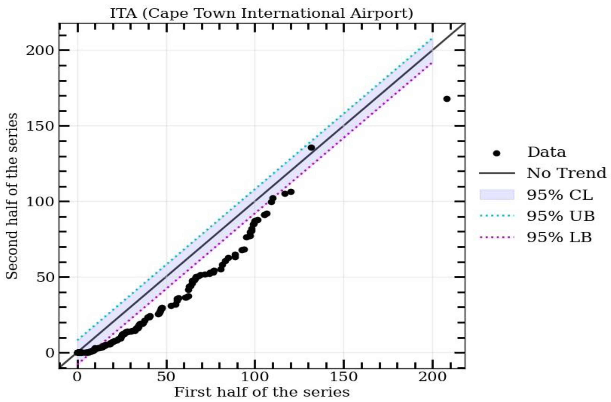
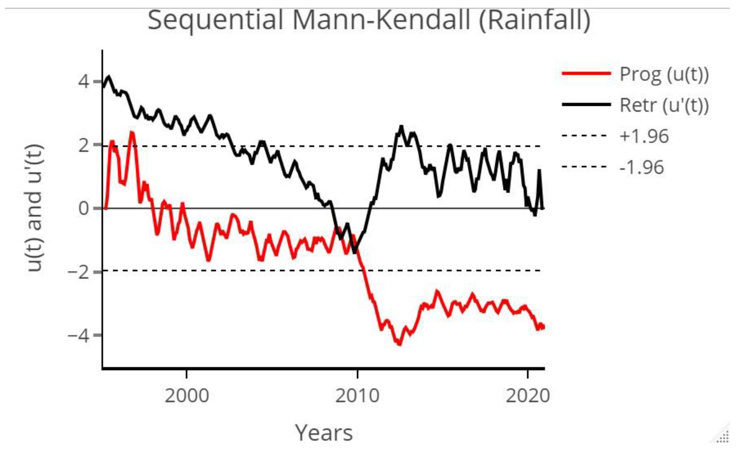
In this study, we utilized innovative trend analysis methods, including the Mann–Kendall test and Sequential Mann–Kendall test, to determine the drought trends in meteorological variables within the basin. The precipitation drought indicator was evaluated in relation to the precipitation data obtained from the weather station at Cape Town International Airport. The ITA, Mann–Kendall test, and SQ-MK trend methods indicated a significant downward trend in rainfall in Cape Town. These findings align with the research conducted by Ndebele et al. [82] and Jury [83]. A study conducted by Ndebele [82] also reported a significant negative trend in rainfall measurements for Cape Town. Additionally, Jury [82] found evidence of a consistent drying trend, faster warming, and declining rainfall, particularly during the winter wet seasons. The SQ-MK findings presented in this research further support the notion of a steady dry trend, which coincided with the El Niño Period of 2015–2017. These results are consistent with the findings of a study conducted by Wolski et al. [84]. We also employed ITA, which complements the MK and SQ-MK tests in terms of trends, and the results reveal the importance of knowing drought conditions. The findings of our study support previous research conducted by Nxumalo et al. [85], Muse et al. [86], and Tladi et al. [87], which emphasize the importance of employing trend analysis in African countries to investigate the impacts of climate change. Trends and predictive models play a crucial role in informing proactive decision making.

According to the statistical indices in Table 4, the models with CEEMDAN performed considerably better than those without, leading to improved forecasting accuracy. These findings are consistent with previous studies [37,47,88,89,90,91], which emphasized the enhanced forecasting accuracy of employing hybrid drought forecasting models in comparison to stand-alone models. For instance, Ding et al. [37] proposed a hybrid model based on complementary ensemble empirical mode decomposition (CEEMD) and long short-term memory (LSTM) to improve the accuracy of drought prediction in the Xinjiang Uygur Autonomous Region in China. A comparison of their results revealed that CEEMD was able to improve the forecasting accuracy of the hybrid model, as evidenced by the decreasing mean square error with increasing timescale, and the gradual improvement of the CEEMD-LSTM models. The hybrid CEEMD-LSTM model outperformed the LSTM model with RMSE values of 0.815, 0.578, 0.378, 0.291, 0.219, and 0.152 for SPI-1, SPI-3, SPI-6, SPI-9, SPI-12, and SPI-24, respectively. Xu et al. [47] explored the strengths of autoregressive integrated moving average (ARIMA) and complementary ensemble empirical mode decomposition (CEEMD) to predict drought using 60 years of monthly precipitation data from 1960 to 2019 for the Ningxia Hui Autonomous Region. The results revealed that the CEEMD–ARIMA model had lower MAE and RMSE values compared to the ARIMA model at all timescales. Additionally, the NSE, KGE, and WI values were higher for the CEEMD–ARIMA model, indicating higher prediction accuracy and suitability for predicting a multiscale SPI. Salisu and Shabriet [89] proposed a hybrid Wavelet–ARIMA model and examined its ability to forecast drought using SPI data from January 1954 to December 2008. The comparison of their results showed that the Wavelet improved the forecasting accuracy of the hybrid model, as the mean square error decreased by an average value of 43%. Rezaiy and Shabri [90] combined the Support Vector Machine (SVM) model with ensemble empirical mode decomposition (EEMD) to present a novel method for drought prediction using monthly precipitation data from Bamyan province in Central Afghanistan, spanning the period January 1970 to December 2019. The results demonstrated that the EEMD-SVM technique significantly improved drought forecasting accuracy, especially for mid- and long-term SPIs. For example, in the testing period, SPI 9 yielded an RMSE of 0.1632, MAE of 0.1208, and R² of 0.9357, while for SPI 12, the RMSE was 0.1078, MAE was 0.0745, and $R^2$ was 0.9141. These results indicate that the EEMD-SVM technique outperformed conventional ARIMA and SVM models, achieving the best criteria with the lowest RMSE and MAE values and the highest $R^2$ value.

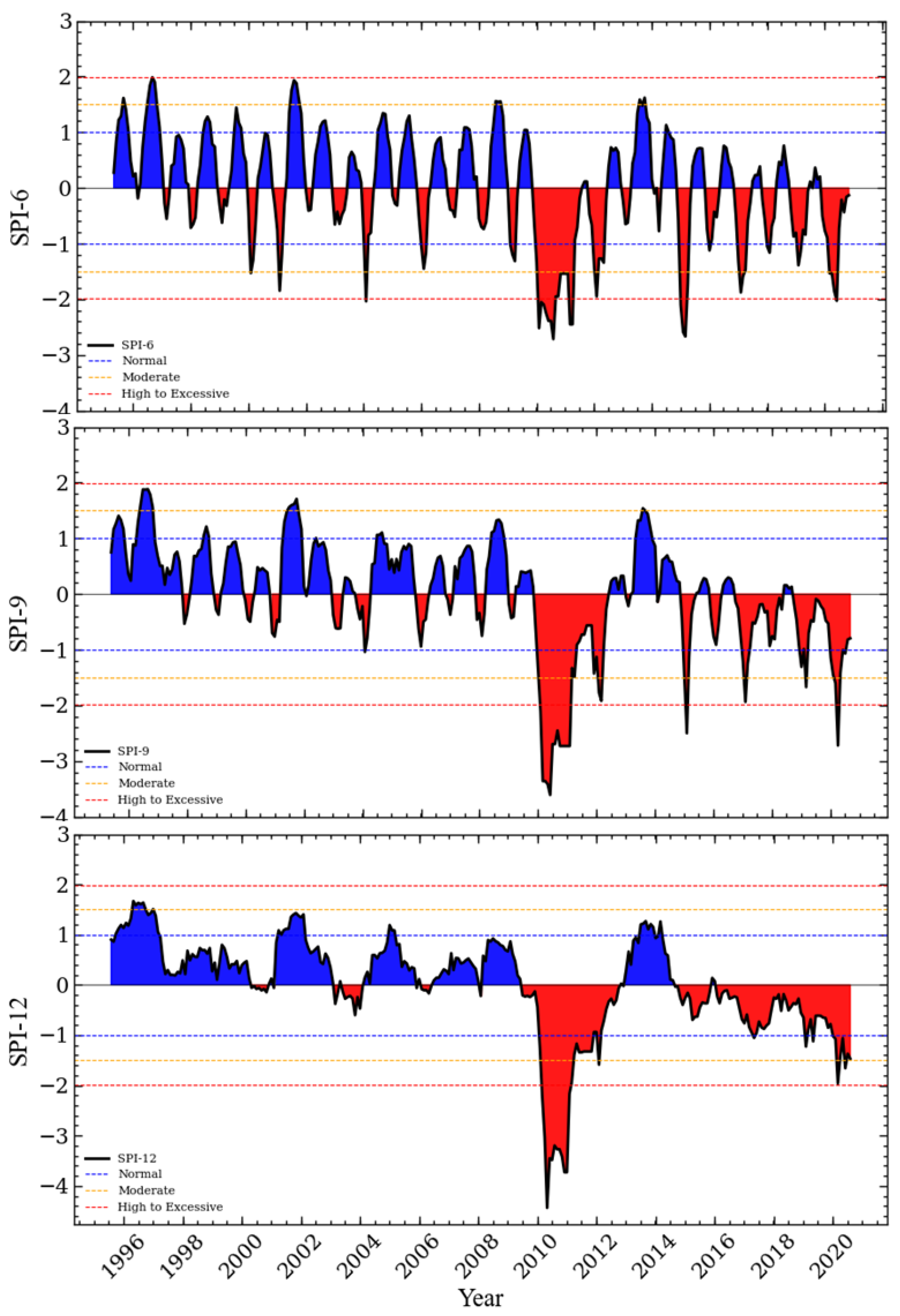
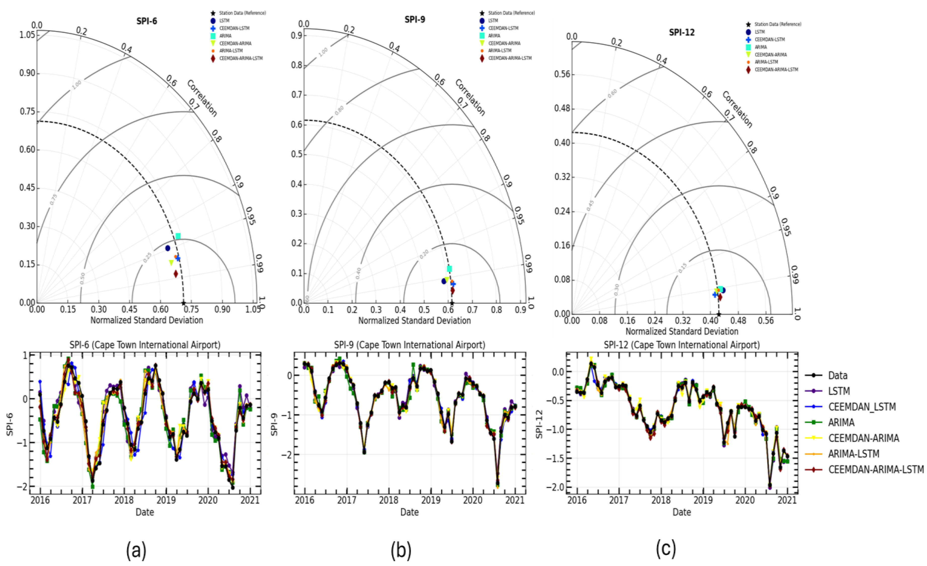
Based on a comparative analysis of this study’s findings with previous research, it is evident that the SPI forecasting results indicate that the hybrid model (CEEMDAN-ARIMA-LSTM) consistently outperformed all other models across all SPI timescales in terms of prediction accuracy. The RMSE of the CEEMDAN-ARIMA-LSTM hybrid model is 0.121, 0.044, and 0.042 for SPI-6, SPI-9, and SPI-12, respectively. The $R^2$ for this hybrid model is 0.972, 0.991, and 0.955, for SPI-6, SPI-9, and SPI-12, respectively. This indicates that this is the most suitable model for forecasting long-term drought conditions in Cape Town. Based on the aforementioned discussion and the findings of this study, our work provides valuable insights into the use of the hybrid CEEMDAN-ARIMA-LSTM model for forecasting meteorological drought.

5. Conclusions

In the present study, the Mann–Kendall (MK) test and the innovative trend analysis (ITA) method were utilized to analyze the trends in monthly rainfall total data from Cape Town International Airport, South Africa, for the period from 1995 to 2020. The results of the MK and MMK tests indicated a significant decreasing trend in rainfall at a 95% significance level. These findings were further supported by the ITA results, with most data points falling below the 1:1 line, indicating a downward trend. Both the SQ-MK and ITA methods indicate a significant downward trend of rainfall in the study area for most of the years studied. A recovery of the downward trend seems to be observed during the period after the 2014–2016 strong El Niño years. Moreover, this study used rainfall data to compute the SPI and used this data train and forecast the SPI data at multiscale using ARIMA and LSTM. To achieve accurate SPI forecasts, the CEEMDAN signal processing algorithm was integrated with the ARIMA, LSTM, and ARIMA-LSTM hybrid model. A comprehensive comparative analysis of the prediction outcomes was conducted (see Figure 10 and Table 4). The results revealed that all the models produced a good performance in predicting the SPI in all the timescales. The performance steadily increased as the timescale increased, presumably because of the lower noise levels for higher SPI timescales. Throughout multiple timescales, the CEEMDAN combined hybrid model consistently outperformed the individual models. Specifically, for SPI12, the hybrid model exhibited RMSE values exceeding 0.97, highlighting CEEMDAN’s ability to handle nonstationary and nonlinear data characteristics, thereby improving predictability. Additionally, as depicted in Figure 10, the drought index predictions derived from the hybrid CEEMDAN-ARIMA-LSTM model are reported to have a superior prediction accuracy compared to other models across all timescales. It is evident that the combination of CEEMDAN with ARIMA, LSTM, and ARIMA-LSTM has the potential to significantly enhance the accuracy of meteorological drought forecasting. Based on the results and discussion, the main conclusion of this study is that integrating CEEMDAN and ARIMA with LSTM resulted in a highly valuable tool for meteorological drought forecasting, which could be key for early warning systems. This could be useful for planning and policy decisions related to agricultural production and tourism management. Furthermore, analyzing climate parameters can help predict climate changes, especially drought and abnormal wet spells. And future investigations should explore the predictability of the standardized precipitation evapotranspiration index (SPEI) to assess the applicability of the combined model.

References

1. Fang, O.; Zhang, Q.-B.; Vitasse, Y.; Zweifel, R.; Cherubini, P. The frequency and severity of past droughts shape the drought sensitivity of juniper trees on the Tibetan plateau. For. Ecol. Manag. 2021, 486, 118968. [Google Scholar] [CrossRef]
2. Murgatroyd, A.; Gavin, H.; Becher, O.; Coxon, G.; Hunt, D.; Fallon, E.; Wilson, J.; Cuceloglu, G.; Hall, J.W. Strategic analysis of the drought resilience of water supply systems. Philos. Trans. R. Soc. A 2022, 380, 20210292. [Google Scholar] [CrossRef]
3. Garrick, D.; De Stefano, L.; Yu, W.; Jorgensen, I.; O’Donnell, E.; Turley, L.; Aguilar-Barajas, I.; Dai, X.; de Souza Leão, R.; Punjabi, B.; et al. Rural water for thirsty cities: A systematic review of water reallocation from rural to urban regions. Environ. Res. Lett. 2019, 14, 043003. [Google Scholar] [CrossRef]
4. Vorosmarty, C.J.; Green, P.; Salisbury, J.; Lammers, R.B. Global water resources: Vulnerability from climate change and population growth. Science 2000, 289, 284–288. [Google Scholar] [CrossRef]
5. Hall, J.W.; Grey, D.; Garrick, D.; Fung, F.; Brown, C.; Dadson, S.J.; Sadoff, C.W. Coping with the curse of freshwater variability. Science 2014, 346, 429–430. [Google Scholar] [CrossRef] [PubMed]
6. Murgatroyd, A.; Hall, J.W. Regulation of freshwater use to restore ecosystems resilience. Clim. Risk Manag. 2021, 32, 100303. [Google Scholar] [CrossRef]
7. Jin, L.; Whitehead, P.G.; Bussi, G.; Hirpa, F.; Taye, M.T.; Abebe, Y.; Charles, K. Natural and anthropogenic sources of salinity in the Awash River and Lake Beseka (Ethiopia): Modelling impacts of climate change and lake-river interactions. J. Hydrol. Reg. Stud. 2021, 36, 100865. [Google Scholar] [CrossRef]
8. Hall, J.W.; Borgomeo, E.; Bruce, A.; Di Mauro, M.; Mortazavi-Naeini, M. Resilience of water resource systems: Lessons from England. Water Secur. 2019, 8, 100052. [Google Scholar] [CrossRef]
9. Ding, Y.; Xu, J.; Wang, X.; Cai, H.; Zhou, Z.; Sun, Y.; Shi, H. Propagation of meteorological to hydrological drought for different climate regions in China. J. Environ. Manag. 2021, 283, 111980. [Google Scholar] [CrossRef]
10. Esfahanian, E.; Nejadhashemi, A.P.; Abouali, M.; Adhikari, U.; Zhang, Z.; Daneshvar, F.; Herman, M.R. Development and evaluation of a comprehensive drought index. J. Environ. Manag. 2017, 185, 31–43. [Google Scholar] [CrossRef]
11. Alley, W.M. The Palmer drought severity index: Limitations and assumptions. J. Clim. Appl. Meteorol. 1984, 23, 1100–1109. [Google Scholar] [CrossRef]
12. Byun, H.R.; Wilhite, D.A. Objective quantification of drought severity and duration. J. Clim. 1999, 12, 2747–2756. [Google Scholar] [CrossRef]
13. Tsakiris, G.; Pangalou, D.; Vangelis, H. Regional drought assessment based on the Reconnaissance Drought Index (RDI). Water Resour. Manag. 2007, 21, 821–833. [Google Scholar] [CrossRef]
14. Beguería, S.; Vicente-Serrano, S.M.; Reig, F.; Latorre, B. Vicente-Serrano, Fergus Reig, and Borja Latorre. Standardized precipitation evapotranspiration index (SPEI) revisited: Parameter fitting, evapotranspiration models, tools, datasets and drought monitoring. Int. J. Climatol. 2014, 34, 3001–3023. [Google Scholar] [CrossRef]
15. Lyon, B.; Barnston, A.G. ENSO and the spatial extent of interannual precipitation extremes in tropical land areas. J. Clim. 2005, 18, 5095–5109. [Google Scholar] [CrossRef]
16. Erhardt, T.M.; Czado, C. Standardized drought indices: A novel univariate and multivariate approach. J. R. Stat. Soc. Ser. C Appl. Stat. 2018, 67, 643–664. [Google Scholar] [CrossRef]
17. Zargar, A.; Sadiq, R.; Naser, B.; Khan, F.I. A review of drought indices. Environ. Rev. 2011, 19, 333–349. [Google Scholar] [CrossRef]
18. McKee, T.B.; Doesken, N.J.; Kleist, J. The relationship of drought frequency and duration to time scales. In Proceedings of the 8th Conference on Applied Climatology, Anaheim, CA, USA, 17–22 January 1993; Volume 17, pp. 179–183. [Google Scholar]
19. Hayes, M.; Svoboda, M.; Wall, N.; Widhalm, M. The Lincoln declaration on drought indices: Universal meteorological drought index recommended. Bull. Am. Meteorol. Soc. 2011, 92, 485–488. [Google Scholar] [CrossRef]
20. Svoboda, M.D.; Fuchs, B.A. Handbook of Drought Indicators and Indices; World Meteorological Organization: Geneva, Switzerland, 2016; Volume 2. [Google Scholar]
21. Latifoğlu, L.; Özger, M. A novel approach for high-performance estimation of SPI data in drought prediction. Sustainability 2023, 15, 14046. [Google Scholar] [CrossRef]
22. Wu, H.; Hayes, M.J.; Weiss, A.; Hu, Q.I. An evaluation of the Standardized Precipitation Index, the China-Z Index and the statistical Z-Score. Int. J. Climatol. 2001, 21, 745–758. [Google Scholar] [CrossRef]
23. Choubin, B.; Malekian, A.; Gloshan, M. Application of several data-driven techniques to predict a standardized precipitation index. Atmósfera 2016, 29, 121–128. [Google Scholar] [CrossRef]
24. Hosseini-Moghari, S.M.; Araghinejad, S.; Azarnivand, A. Drought forecasting using data-driven methods and an evolutionary algorithm. Model. Earth Syst. Environ. 2017, 3, 1675–1689. [Google Scholar] [CrossRef]
25. Aghelpour, P.; Kisi, O.; Varshavian, V. Multivariate drought forecasting in short-and long-term horizons using MSPI and data-driven approaches. J. Hydrol. Eng. 2021, 26, 04021006. [Google Scholar] [CrossRef]
26. Elbeltagi, A.; AlThobiani, F.; Kamruzzaman, M.; Shaid, S.; Roy, D.K.; Deb, L.; Islam, M.M.; Kundu, P.K.; Rahman, M.M. Estimating the standardized precipitation evapotranspiration index using data-driven techniques: A regional study of Bangladesh. Water 2022, 14, 1764. [Google Scholar] [CrossRef]
27. Pande, C.B.; Costache, R.; Sammen, S.S.; Noor, R.; Elbeltagi, A. Combination of data-driven models and best subset regression for predicting the standardized precipitation index (SPI) at the Upper Godavari Basin in India. Theor. Appl. Climatol. 2023, 152, 535–558. [Google Scholar] [CrossRef]
28. Noh, S.; Lee, S. Forecasting Meteorological Drought Conditions in South Korea Using a Data-Driven Model with Lagged Global Climate Variability. Sustainability 2024, 16, 6485. [Google Scholar] [CrossRef]
29. Khan, M.M.H.; Muhammad, N.S.; El-Shafie, A. Wavelet based hybrid ANN-ARIMA models for meteorological drought forecasting. J. Hydrol. 2020, 590, 125380. [Google Scholar] [CrossRef]
30. Han, P.; Wang, P.; Tian, M.; Zhang, S.; Liu, J.; Zhu, D. Application of the ARIMA models in drought forecasting using the standardized precipitation index. In Computer and Computing Technologies in Agriculture VI, Proceedings of the 6th IFIP WG 5.14 International Conference, CCTA 2012, Zhangjiajie, China, 19–21 October 2012; Revised Selected Papers, Part I 6; Springer: Berlin/Heidelberg, Germany, 2013; pp. 352–358. [Google Scholar]
31. Tan, Y.X.; Ng, J.L.; Huang, Y.F. A review on drought index forecasting and their modelling approaches. Arch. Comput. Methods Eng. 2023, 30, 1111–1129. [Google Scholar] [CrossRef]
32. Achite, M.; Elshaboury, N.; Jehanzaib, M.; Vishwakarma, D.K.; Pham, Q.B.; Anh, D.T.; Abdelkader, E.M.; Elbeltagi, A. Performance of machine learning techniques for meteorological drought forecasting in the Wadi Mina Basin, Algeria. Water 2023, 15, 765. [Google Scholar] [CrossRef]
33. Liu, M.-D.; Ding, L.; Bai, Y.-L. Application of hybrid model based on empirical mode decomposition, novel recurrent neural networks and the ARIMA to wind speed prediction. Energy Convers. Manag. 2021, 233, 113917. [Google Scholar] [CrossRef]
34. Poornima, S.; Pushpalatha, M. Drought prediction based on SPI and SPEI with varying timescales using LSTM recurrent neural network. Soft Comput. 2019, 23, 8399–8412. [Google Scholar] [CrossRef]
35. Dikshit, A.; Pradhan, B.; Alamri, A.M. Long lead time drought forecasting using lagged climate variables and a stacked long short-term memory model. Sci. Total Environ. 2021, 755, 142638. [Google Scholar] [CrossRef] [PubMed]
36. Balti, H.; Abbes, A.B.; Mellouli, N.; Sang, Y.; Farah, I.R.; Lamolle, M.; Zhu, Y. Big data based architecture for drought forecasting using LSTM, ARIMA, and Prophet: Case study of the Jiangsu Province, China. In Proceedings of the 2021 International Congress of Advanced Technology and Engineering (ICOTEN), Virtual Conference, 4–5 July 2021; IEEE: New York, NY, USA, 2021; pp. 1–8. [Google Scholar]
37. Ding, Y.; Yu, G.; Tian, R.; Sun, Y. Application of a hybrid CEEMD-LSTM model based on the standardized precipitation index for Drought forecasting: The case of the Xinjiang Uygur Autonomous Region, China. Atmosphere 2022, 13, 1504. [Google Scholar] [CrossRef]
38. Wang, Z.-Y.; Qiu, J.; Li, F.-F. Hybrid models combining EMD/EEMD and ARIMA for Long-term streamflow forecasting. Water 2018, 10, 853. [Google Scholar] [CrossRef]
39. Mathivha, F.; Sigauke, C.; Chikoore, H.; Odiyo, J. Short-term and medium-term drought forecasting using generalized additive models. Sustainability 2020, 12, 4006. [Google Scholar] [CrossRef]
40. Guoyang, Z.; Xinjun, T.; Tian, W.; Yuting, X.I.E.; Xiaomei, M.O. Drought Prediction Based on Artificial Neural Network and Support Vector Machine. Pearl River 2021, 42, 1. [Google Scholar]
41. Wu, G.; Zhang, J.; Xue, H. Long-Term Prediction of Hydrometeorological Time Series Using a PSO-Based Combined Model Composed of EEMD and LSTM. Sustainability 2023, 15, 13209. [Google Scholar] [CrossRef]
42. Rezaiy, R.; Shabri, A. An innovative hybrid W-EEMD-ARIMA model for drought forecasting using the standardized precipitation index. In Natural Hazards; Springer: Berlin/Heidelberg, Germany, 2024; pp. 1–30. [Google Scholar]
43. Belayneh, A.; Adamowski, J.; Khalil, B.; Quilty, J. Coupling machine learning methods with wavelet transforms and the bootstrap and boosting ensemble approaches for drought prediction. Atmos. Res. 2016, 172, 37–47. [Google Scholar] [CrossRef]
44. Rezaiy, R.; Shabri, A. Drought forecasting using W-ARIMA model with standardized precipitation index. J. Water Clim. Chang. 2023, 14, 3345–3367. [Google Scholar] [CrossRef]
45. Coşkun, Ö.; Citakoglu, H. Prediction of the standardized precipitation index based on the long short-term memory and empirical mode decomposition-extreme learning machine models: The Case of Sakarya, Türkiye. Phys. Chem. Earth Parts A/B/C 2023, 131, 103418. [Google Scholar] [CrossRef]
46. Libanda, B.; Nkolola, N.B. An ensemble empirical mode decomposition of consecutive dry days in the Zambezi Riparian Region: Implications for water management. Phys. Chem. Earth Parts A/B/C 2022, 126, 103147. [Google Scholar] [CrossRef]
47. Xu, D.; Ding, Y.; Liu, H.; Zhang, Q.; Zhang, D. Applicability of a CEEMD–ARIMA Combined Model for Drought Forecasting: A Case Study in the Ningxia Hui Autonomous Region. Atmosphere 2022, 13, 1109. [Google Scholar] [CrossRef]
48. Hao, Z.; Singh, V.P.; Xia, Y. Seasonal drought prediction: Advances, challenges, and future prospects. Rev. Geophys. 2018, 56, 108–141. [Google Scholar] [CrossRef]
49. Adnan, R.M.; Mostafa, R.R.; Islam AR, M.T.; Gorgij, A.D.; Kuriqi, A.; Kisi, O. Improving drought modeling using hybrid random vector functional link methods. Water 2021, 13, 3379. [Google Scholar] [CrossRef]
50. Wu, X.; Zhou, J.; Yu, H.; Liu, D.; Xie, K.; Chen, Y.; Hu, J.; Sun, H.; Xing, F. The development of a hybrid wavelet-ARIMA-LSTM model for precipitation amounts and drought analysis. Atmosphere 2021, 12, 74. [Google Scholar] [CrossRef]
51. Mann, H.B. Nonparametric tests against trend. Econometrica 1945, 13, 245–259. [Google Scholar] [CrossRef]
52. Kendall, M.G. Rank Correlation Methods; Griffin: London, UK, 1975. [Google Scholar]
53. Seenu, P.Z.; Jayakumar, K.V. Comparative study of innovative trend analysis technique with Mann-Kendall tests for extreme rainfall. Arab. J. Geosci. 2021, 14, 536. [Google Scholar]
54. Körük, A.E.; Kankal, M.; Yıldız, M.B.; Akçay, F.; Şan, M.; Nacar, S. Trend analysis of precipitation using innovative approaches in northwestern Turkey. Phys. Chem. Earth Parts A/B/C 2023, 131, 103416. [Google Scholar] [CrossRef]
55. Mbatha, N.; Xulu, S. Time series analysis of MODIS-Derived NDVI for the Hluhluwe-Imfolozi Park, South Africa: Impact of recent intense drought. Climate 2018, 6, 95. [Google Scholar] [CrossRef]
56. Onoz, B.; Bayazit, M. The power of statistical tests for trend detection. Turk. J. Eng. Environ. Sci. 2003, 27, 247–251. [Google Scholar]
57. Othman, M.A.; Zakaria, N.A.; Ghani, A.A.; Chang, C.K.; Chan, N.W. Analysis of trends of extreme rainfall events using Mann Kendall test: A case study in Pahang and Kelantan river basins. J. Teknol. 2016, 78. [Google Scholar] [CrossRef]
58. Hamed, K.H.; Rao, A.R. A modified Mann-Kendall trend test for autocorrelated data. J. Hydrol. 1998, 204, 182–196. [Google Scholar] [CrossRef]
59. Kumar, S.; Machiwal, D.; Dayal, D. Spatial modelling of rainfall trends using satellite datasets and geographic information system. Hydrol. Sci. J. 2017, 62, 1636–1653. [Google Scholar] [CrossRef]
60. Singh, R.N.; Sah, S.; Das, B.; Potekar, S.; Chaudhary, A.; Pathak, H. Innovative trend analysis of spatio-temporal variations of rainfall in India during 1901–2019. Theor. Appl. Climatol. 2021, 145, 821–838. [Google Scholar] [CrossRef]
61. Sneyers, R. On the Statistical Analysis of Series of Observations; Technical Note No. 143, WMO No. 415; World Meteorological Organization: Geneva, Switzerland, 1991; p. 192. [Google Scholar]
62. Bisai, D.; Chatterjee, S.; Khan, A. Detection of recognizing events in lower atmospheric temperature time series (1941–2010) of Midnapore Weather Observatory, West Bengal, India. J. Environ. Earth Sci. 2014, 4, 61–66. [Google Scholar]
63. Şen, Z. Innovative trend analysis methodology. J. Hydrol. Eng. 2012, 17, 1042–1046. [Google Scholar] [CrossRef]
64. Paulo, A.A.; Pereira, L.S. Prediction of SPI drought class transitions using Markov chains. Water Resour. Manag. 2007, 21, 1813–1827. [Google Scholar] [CrossRef]
65. World Meteorological Organization. WMO Statement on the Status of the Global Climate in 2015; World Meteorological Organization (WMO): Geneva, Switzerland, 2016. [Google Scholar]
66. Wilhite, D.A.; Hayes, M.J.; Knutson, C.; Smith, K.H. Planning for drought: Moving from crisis to risk management1. JAWRA J. Am. Water Resour. Assoc. 2000, 36, 697–710. [Google Scholar] [CrossRef]
67. Zhou, H.; Liu, Y. SPI based meteorological drought assessment over a humid basin: Effects of processing schemes. Water 2016, 8, 373. [Google Scholar] [CrossRef]
68. Zhang, X.; Peng, Y.; Zhang, C.; Wang, B. Are hybrid models integrated with data preprocessing techniques suitable for monthly streamflow forecasting? Some experiment evidences. J. Hydrol. 2015, 530, 137–152. [Google Scholar] [CrossRef]
69. Koudahe, K.; Kayode, A.J.; Samson, A.O.; Adebola, A.A.; Djaman, K. Trend analysis in standardized precipitation index and standardized anomaly index in the context of climate change in Southern Togo. Atmos. Clim. Sci. 2017, 7, 401. [Google Scholar] [CrossRef]
70. Nourani, V.; Alami, M.T.; Vousoughi, F.D. Wavelet-entropy data pre-processing approach for ANN-based groundwater level modeling. J. Hydrol. 2015, 524, 255–269. [Google Scholar] [CrossRef]
71. Lloyd-Hughes, B.; Saunders, M.A. A drought climatology for Europe. Int. J. Climatol. 2002, 22, 1571–1592. [Google Scholar] [CrossRef]
72. Torres, M.E.; Colominas, M.A.; Schlotthauer, G.; Flandrin, P. A complete ensemble empirical mode decomposition with adaptive noise. In Proceedings of the 2011 IEEE International Conference on Acoustics, Speech and Signal Processing (ICASSP), Prague, Czech Republic, 22–27 May 2011; IEEE: New York, NY, USA, 2011; pp. 4144–4147. [Google Scholar]
73. Box, G.E.; Jenkin, G.M.; Wisconsin University Madison Department of Statistics. Time Series Analysis Forecasting and Control; Wiley: Hoboken, NJ, USA, 1970. [Google Scholar]
74. Sharma, R.R.; Kumar, M.; Maheshwari, S.; Ray, K.P. EVDHM-ARIMA-based time series forecasting model and its application for COVID-19 cases. IEEE Trans. Instrum. Meas. 2020, 70, 6502210. [Google Scholar] [CrossRef]
75. El-Dakak, A.M.; Saleh, O.K.; Mosad, K.; Elnikhely, E.A. Drought forecast using ARIMA model for the standardized precipitation index (SPI) and precipitation data. Int. J. Civ. Eng. Technol. 2021, 12, 63–79. [Google Scholar]
76. Hochreiter, S.; Schmidhuber, J. Long short-term memory. Neural Comput. 1997, 9, 1735–1780. [Google Scholar] [CrossRef] [PubMed]
77. Calverley, C.M.; Walther, S.C. Drought, water management, and social equity: Analyzing Cape Town, South Africa’s water crisis. Front. Water 2022, 4, 910149. [Google Scholar] [CrossRef]
78. Sun, Y.; Liu, J. Aqi prediction based on ceemdan-arma-lstm. Sustainability 2022, 14, 12182. [Google Scholar] [CrossRef]
79. Makridakis, S. Accuracy measures: Theoretical and practical concerns. Int. J. Forecast. 1993, 9, 527–529. [Google Scholar] [CrossRef]
80. Sameen, M.I.; Pradhan, B.; Lee, S. Application of convolutional neural networks featuring Bayesian optimization for landslide susceptibility assessment. Catena 2020, 186, 104249. [Google Scholar] [CrossRef]
81. Sameen, M.I.; Pradhan, B.; Lee, S. Self-learning random forests model for mapping groundwater yield in data-scarce areas. Nat. Resour. Res. 2019, 28, 757–775. [Google Scholar] [CrossRef]
82. Ndebele, N.E.; Grab, S.; Turasie, A. Characterizing rainfall in the south-western Cape, South Africa: 1841–2016. Int. J. Climatol. 2020, 40, 1992–2014. [Google Scholar] [CrossRef]
83. Jury, M.R. Climate trends in the Cape Town area, South Africa. Water SA 2020, 46, 438–447. [Google Scholar]
84. Wolski, P.; Conradie, S.; Jack, C.; Tadross, M. Spatio-temporal patterns of rainfall trends and the 2015–2017 drought over the winter rainfall region of South Africa. Int. J. Climatol. 2021, 41, E1303–E1319. [Google Scholar] [CrossRef]
85. Nxumalo, G.; Bashir, B.; Alsafadi, K.; Bachir, H.; Harsányi, E.; Arshad, S.; Mohammed, S. Meteorological drought variability and its impact on wheat yields across South Africa. Int. J. Environ. Res. Public Health 2022, 19, 16469. [Google Scholar] [CrossRef] [PubMed]
86. Muse, N.M.; Tayfur, G.; Safari, M.J.S. Meteorological drought assessment and trend analysis in Puntland region of Somalia. Sustainability 2023, 15, 10652. [Google Scholar] [CrossRef]
87. Tladi, T.M.; Ndambuki, J.M.; Olwal, T.O.; Rwanga, S.S. Groundwater Level Trend Analysis and Prediction in the Upper Crocodile Sub-Basin, South Africa. Water 2023, 15, 3025. [Google Scholar] [CrossRef]
88. Zhang, X.; Wu, X.; He, S.; Zhao, D. Precipitation forecast based on CEEMD–LSTM coupled model. Water Supply 2021, 21, 4641–4657. [Google Scholar] [CrossRef]
89. Salisu, A.M.; Shabri, A. A hybrid wavelet-ARIMA model for standardized precipitation index drought forecasting. Matematika 2020, 36, 141–156. [Google Scholar] [CrossRef]
90. Rezaiy, R.; Shabri, A. Improving drought prediction accuracy: A hybrid EEMD and support vector machine approach with standardized precipitation index. Water Resour. Manag. 2024, 1–23. [Google Scholar] [CrossRef]
91. Alquraish, M.; Ali Abuhasel, K.; Alqahtani, A.S.; Khadr, M. SPI-based hybrid hidden Markov–GA, ARIMA–GA, and ARIMA–GA–ANN models for meteorological drought forecasting. Sustainability 2021, 13, 12576. [Google Scholar] [CrossRef]
Figure 1. The study area map. Cape Town International Airport location is indicated by a red star.
Water 16 02469 g001
Figure 2. The s schematic representation of the Box–Jenkins methodology application to improve SPI time series forecasting.
Water 16 02469 g002
Figure 3. The basic unit structure diagram of the LSTM single cell.
Water 16 02469 g003
Figure 4. Schematic structure of the developed hybrid CEEMDAN-ARIMA-LSTM model for time series analysis methodology.
Water 16 02469 g004
Figure 5. Time series of the monthly rainfall.
Water 16 02469 g005
Figure 6. Innovative trend analysis of monthly total rainfall data measured at Cape Town International Airport meteorological station, South Africa. The blue shaded area represents the 95% confidence level area.
Water 16 02469 g006
Figure 7. Sequential Mann–Kendall values of the statistics u(t) (red line) and u’(t) (black line) from the Mann–Kendall test for monthly rainfall measured at Cape Town International Airport for the period from 1995 to 2020.
Water 16 02469 g007
Figure 8. Observed SPI values at the 6-, 9-, and 12-month timescales calculated from the rainfall data measured at Cape Point International Airport. The blue and red shades indicate moist and dry conditions.
Water 16 02469 g008
Figure 9. The CEEMDAN decomposition results of SPI-6 sequence. The blue and red shades indicate moist and dry conditions.
Water 16 02469 g009
Figure 10. The time series of observations and forecasts for the SPI prediction (Bottom) and their Taylor diagram plots at different timescales (Top) (a) SPI-6, (b) SPI-9, and (c) SPI-12.
Water 16 02469 g010