
Reconstruction of Lake Level Changes of Groundwater-Fed Lakes in Northeastern Germany Using RapidEye Time Series

Abstract
:1. Introduction
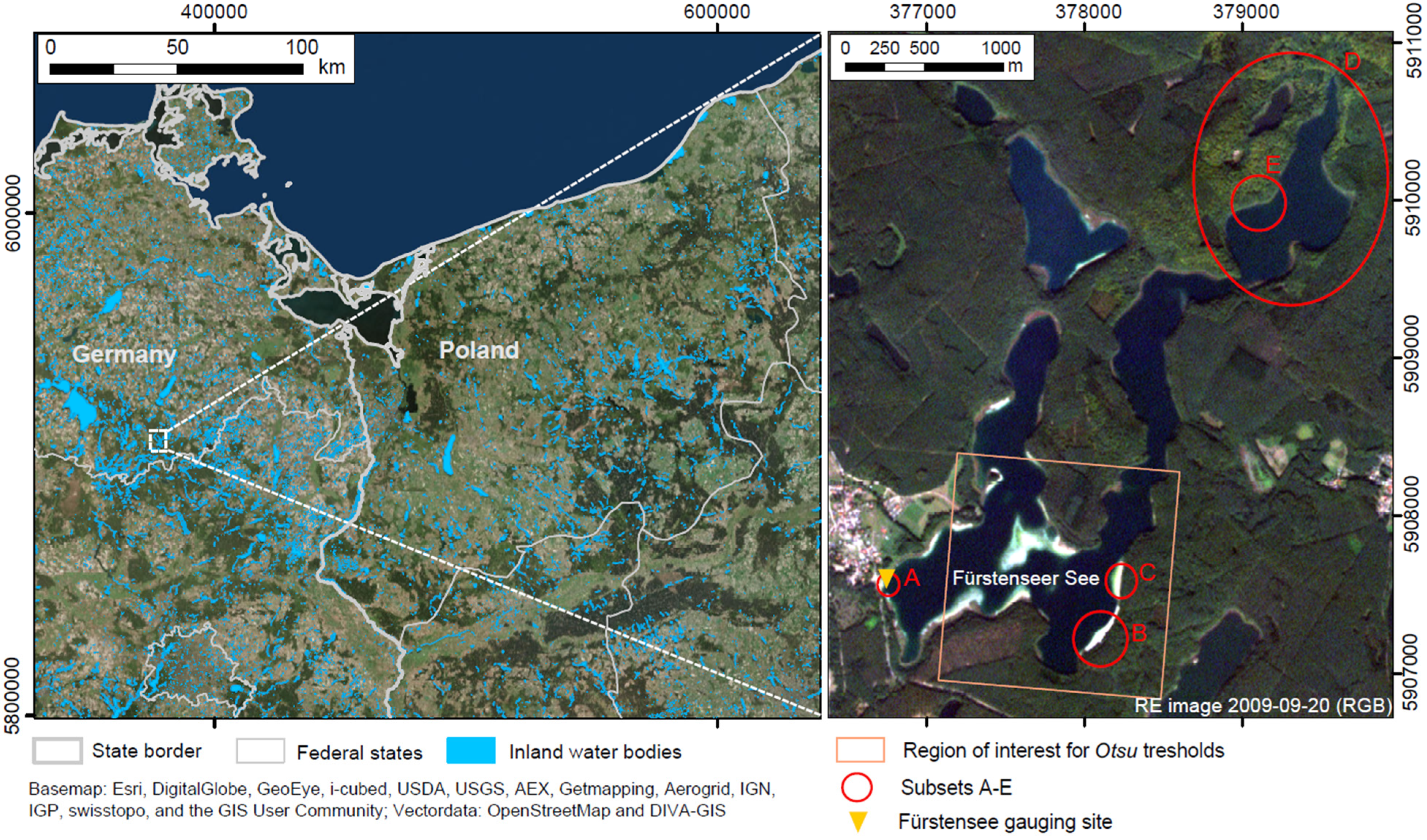
2. Study Area

3. Materials and Methods
3.1. Data Acquisition and Preparation

| Data | Abbreviation | Method/Device | Acquisition Date | Resolution (Accuracy) | Source |
|---|---|---|---|---|---|
| In situ measured lake level | Manual reading at gauging site | monthly since 1987, daily since 2006 | 1 cm | Staatliches Amt für Landwirtschaft und Umwelt Mecklenburgische Seenplatte (MS) [38] | |
| Digital surface model | ATKIS-DGM1 | Pre-processed LiDAR | 1 November 2010 and 15 December 2010 | 1 m (vertical: 0.15–0.2 m) | Landesamt für innere Verwaltung Mecklenburg-Vorpommern [40] |
| Bathymetric point data | Sonar via SIMRAD-Echolot | 7 October 2002 | (Horizontal: 1 m, vertical: 0.1 m) | Ministerium für Landwirtschaft, Umwelt und Verbraucherschutz M-V [37] | |
| In situ measured water-land border | Differential Global Positioning System via Triumph-VS Receiver | 12 August 2014 | (Horizontal RMSE < 1 m) |
| Acquisition Date | Satellite | Sensor | Sensor Viewing Angle (°) | Sun Elevation Angle (SEA) (°) | Lake Levels (m a.s.l.) Measured in situ |
|---|---|---|---|---|---|
| 2009-04-04 | RE-1 | MSI | 0.06 | 42.59 | 63.37 |
| 2009-04-13 | RE-1 | MSI | 13.43 | 45.81 | 63.36 |
| 2009-04-21 | RE-4 | MSI | 6.69 | 48.72 | 63.34 |
| 2009-08-31 | RE-2 | MSI | −3.05 | 45.31 | 63.18 |
| 2009-09-20 | RE-3 | MSI | −2.90 | 37.75 | 63.15 |
| 2010-06-03 | RE-2 | MSI | 17.03 | 59.12 | 63.4 |
| 2010-06-17 | RE-2 | MSI | 20.46 | 60.06 | 63.39 |
| 2010-07-03 | RE-3 | MSI | 3.68 | 59.74 | 63.34 |
| 2010-07-19 | RE-5 | MSI | 10.38 | 57.56 | 63.29 |
| 2010-09-22 | RE-3 | MSI | 3.53 | 37.05 | 63.32 |
| 2010-10-04 | RE-1 | MSI | 13.16 | 32.40 | 63.31 |
| 2011-04-20 | RE-3 | MSI | −2.94 | 48.26 | 63.54 |
| 2011-05-07 | RE-1 | MSI | 3.49 | 53.54 | 63.51 |
| 2011-05-11 | RE-5 | MSI | −3.18 | 54.59 | 63.5 |
| 2011-05-30 | RE-5 | MSI | −2.95 | 58.50 | 63.52 |
| 2011-06-04 | RE-5 | MSI | −9.79 | 59.11 | 63.51 |
| 2011-06-27 | RE-5 | MSI | 13.60 | 60.10 | 63.53 |
| 2011-09-24 | RE-3 | MSI | 6.88 | 36.34 | 63.7 |
| 2011-10-02 | RE‑1 | MSI | −2.96 | 33.05 | 63.7 |
| 2011-10-13 | RE-3 | MSI | 7.07 | 29.00 | 63.7 |
| 2011-10-17 | RE-2 | MSI | 3.91 | 27.42 | 63.7 |
| 2011-10-22 | RE-2 | MSI | −6.11 | 25.52 | 63.7 |
| 2011-11-13 | RE-5 | MSI | −6.21 | 18.63 | 63.68 |
| 2012-04-05 | RE-1 | MSI | −9.61 | 43.05 | 63.92 |
| 2012-05-01 | RE-4 | MSI | 10.25 | 52.08 | 63.94 |
| 2012-05-23 | RE-2 | MSI | 10.24 | 57.48 | 63.91 |
| 2012-06-18 | RE-4 | MSI | −2.95 | 60.21 | 63.84 |
| 2012-07-24 | RE-2 | MSI | 7.03 | 56.53 | 63.83 |
| 2012-10-12 | RE-1 | MSI | 10.00 | 29.07 | 63.77 |
| 2012-11-14 | RE-5 | MSI | −6.25 | 18.14 | 63.77 |
| 2014-03-10 | RE-5 | MSI | −5.87 | 32.77 | 63.86 |
| 2014-03-20 | RE-1 | MSI | 6.69 | 36.70 | 63.86 |
| 2014-04-25 | RE-3 | MSI | −13.11 | 49.95 | 63.87 |
| 2014-05-01 | RE-5 | MSI | 0.31 | 51.93 | 63.86 |
| 2014-05-20 | RE‑5 | MSI | 0.34 | 56.82 | 63.84 |
| 2014-08-06 | RE-2 | MSI | 3.54 | 53.44 | 63.76 |
| 2014-09-05 | RE-3 | MSI | −9.77 | 43.52 | 63.72 |
3.2. Method

4. Results
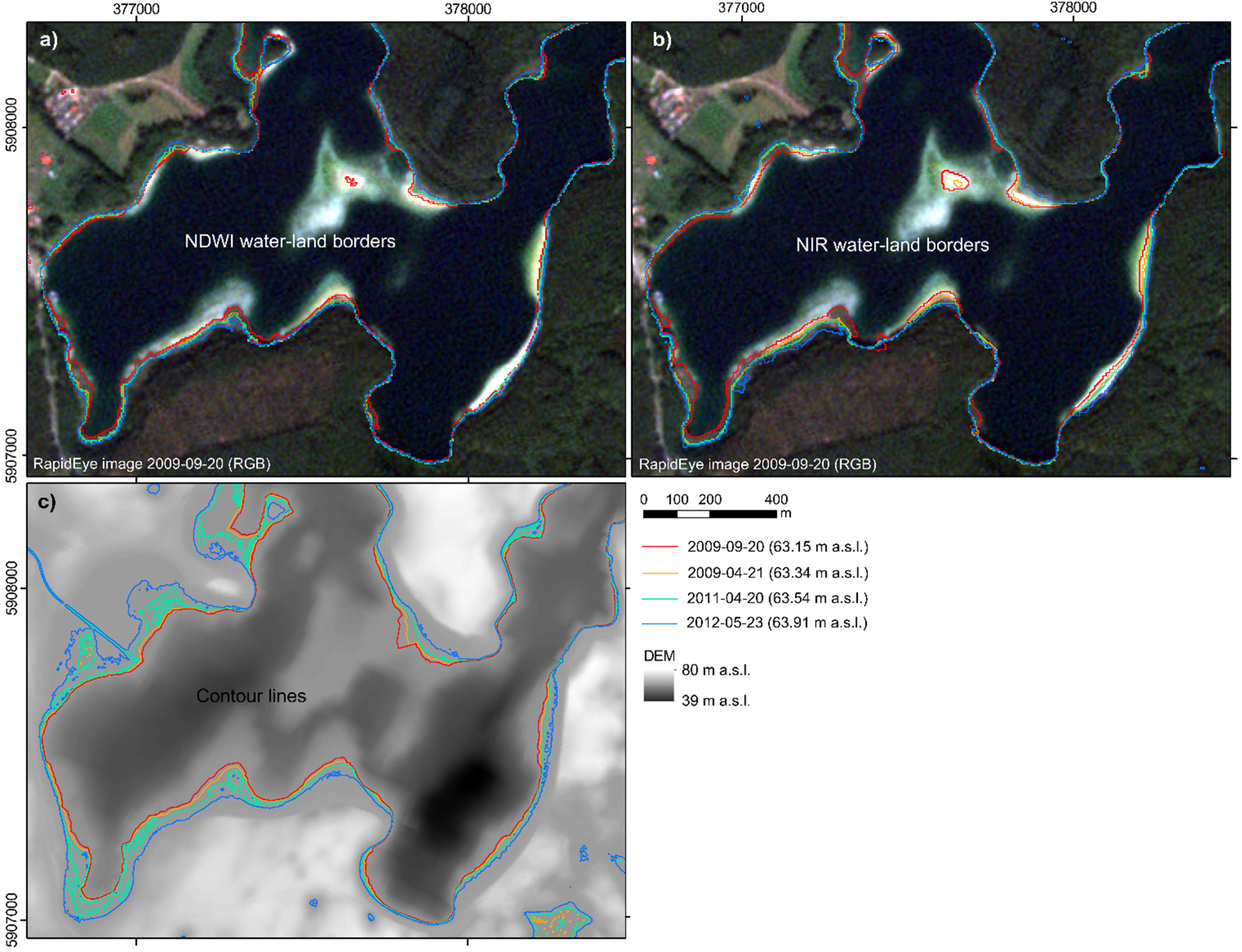
4.1. Automatic Water-Land Border Extraction

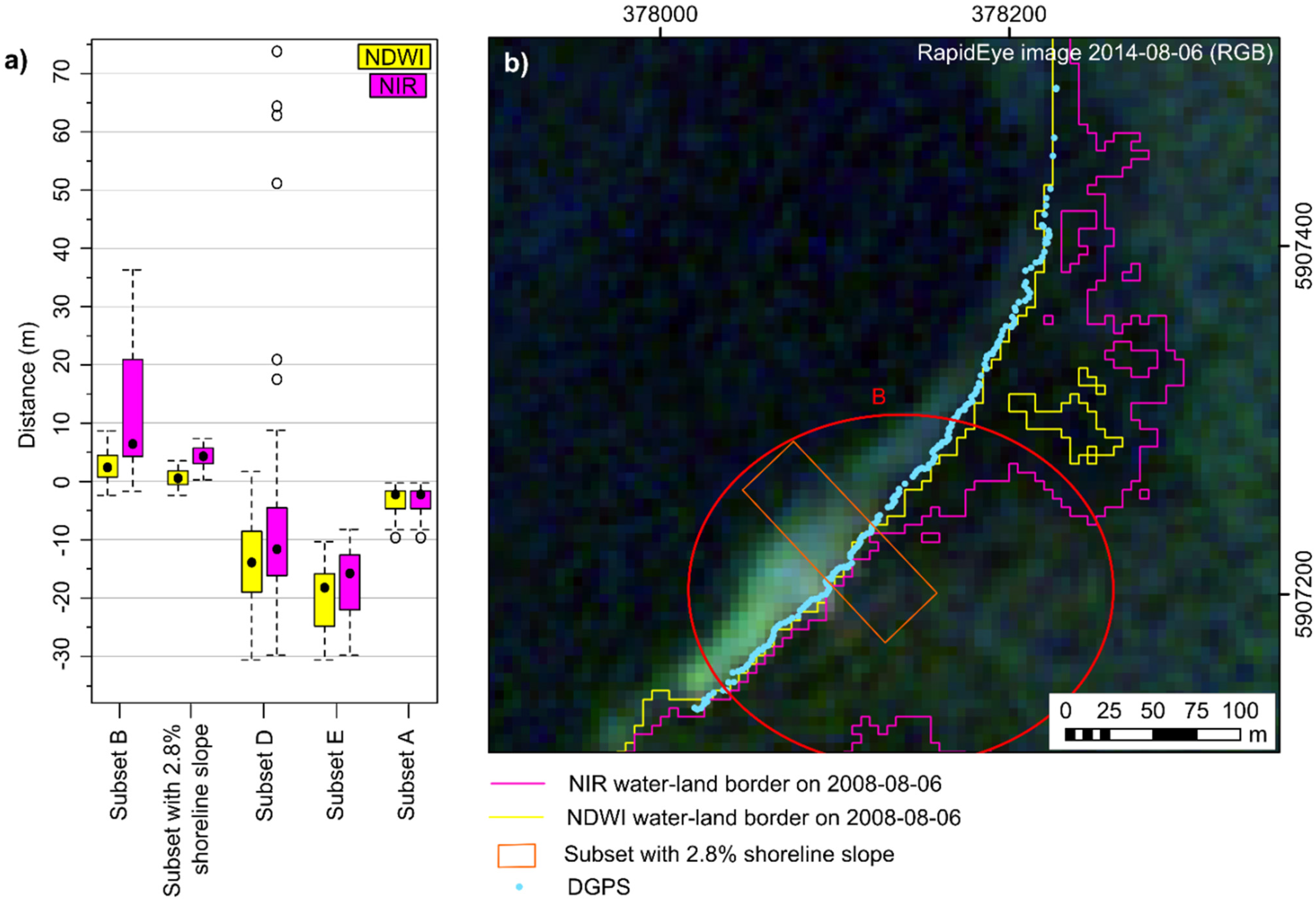
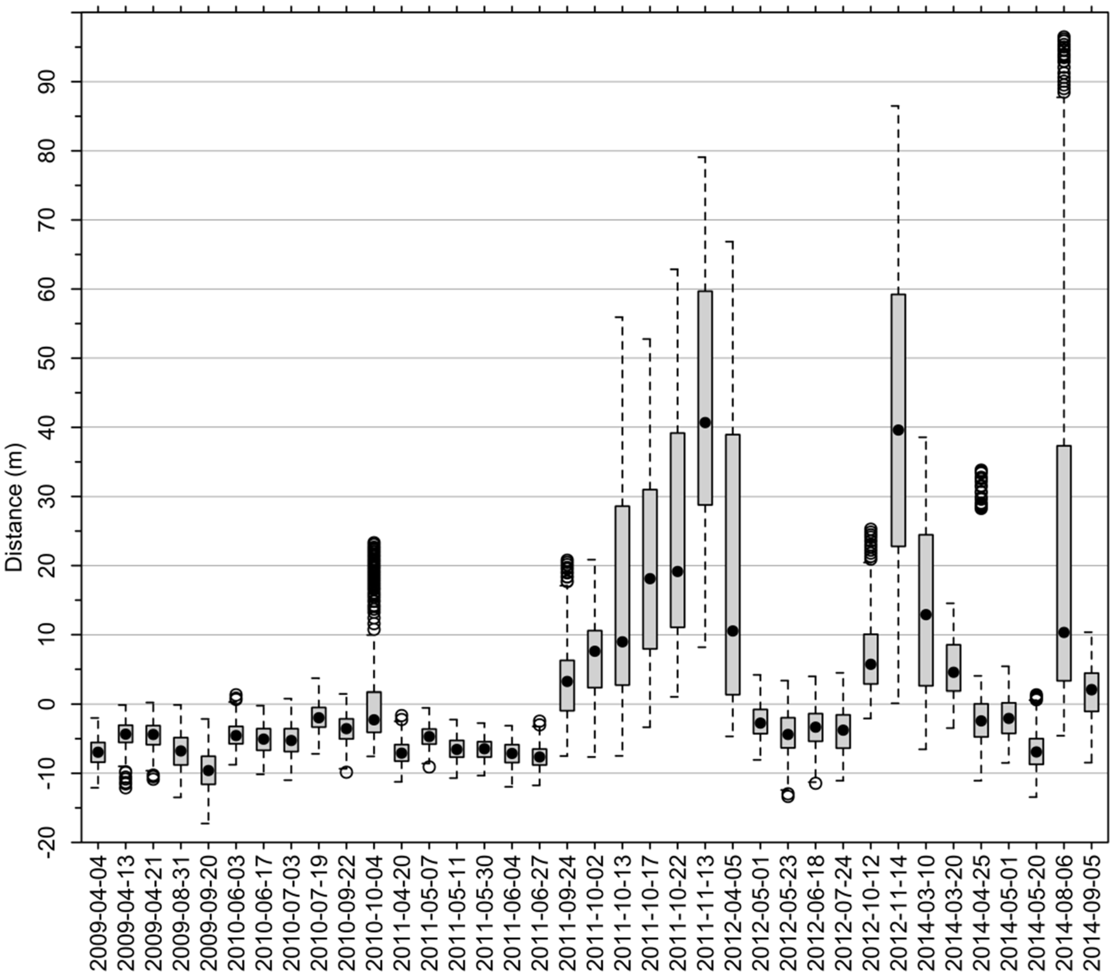
4.2. Shoreline Changes


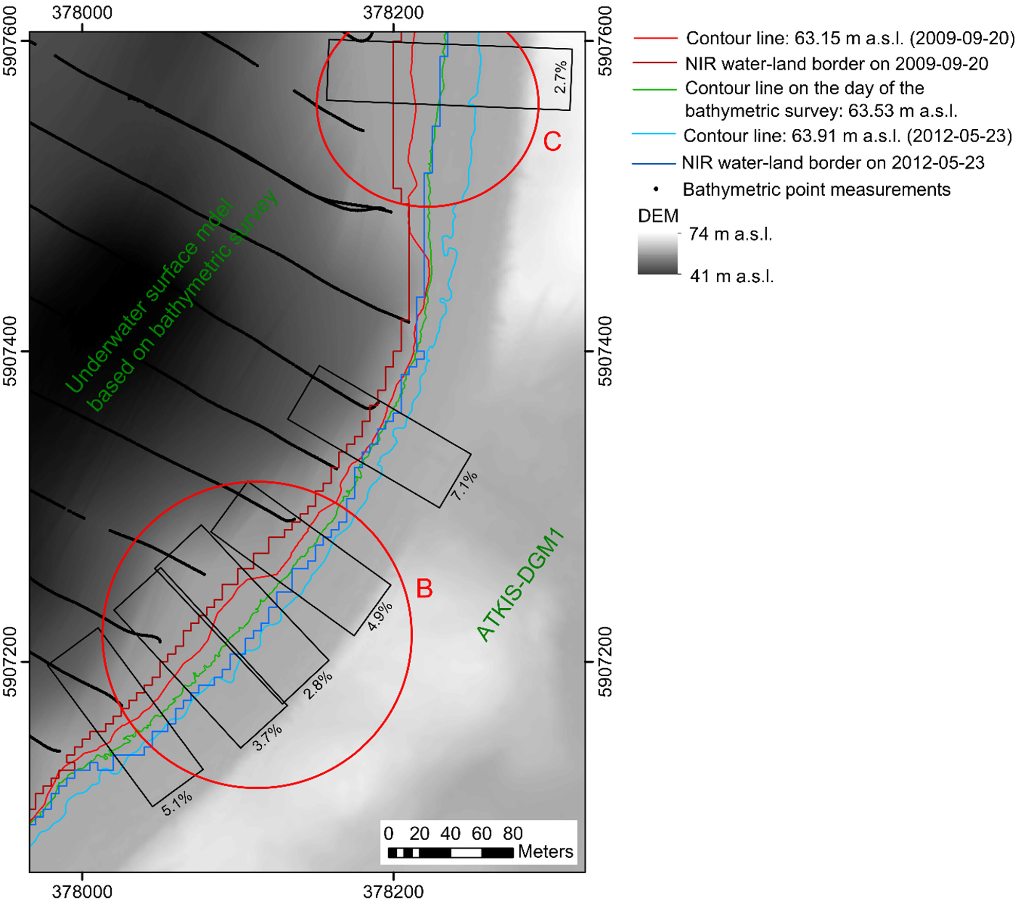
4.3. Subset Selection for Lake Level Reconstruction
| Slope (%) | Distance between Minimum and Maximum NIR Water-Land Border (m) | Distance between Minimum and Maximum Contour Lines (m) | Location (cf. Figure 1 and Figure 3) | Notes |
|---|---|---|---|---|
| 2.7 | 30.1 | 40.2 | Subset C | Trees flooded in August 2014, high lake level |
| 2.8 | 29.6 | 29.0 | Subset B | |
| 3.7 | 29.1 | 21.6 | Subset B | |
| 4.9 | 21.7 | 19.1 | Subset B | |
| 5.1 | 22.2 | 16.3 | Subset B | |
| 7.1 | 10.2 | 10.8 | Subset B | |
| 8.7 | 5.3 | 8.9 | Subset A |
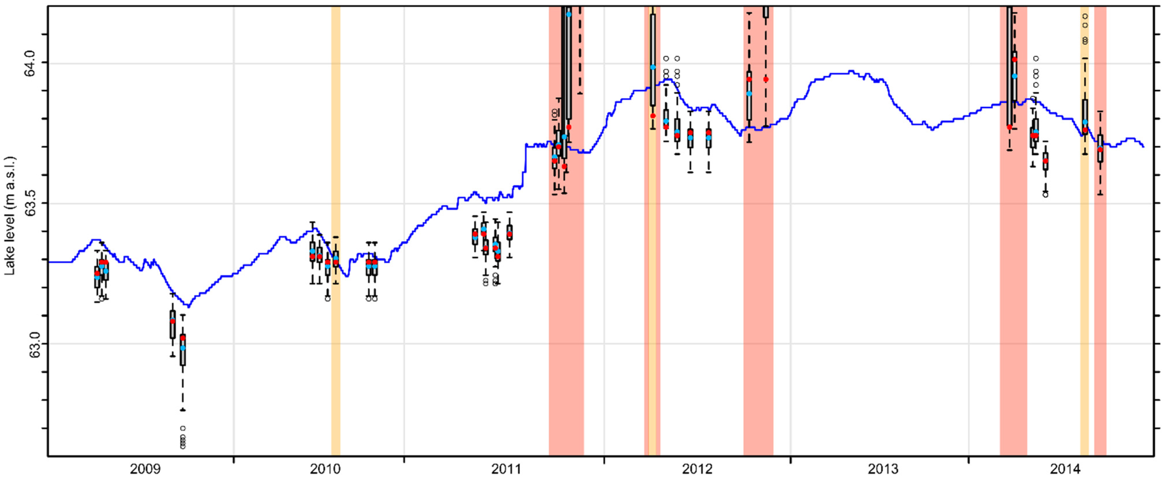
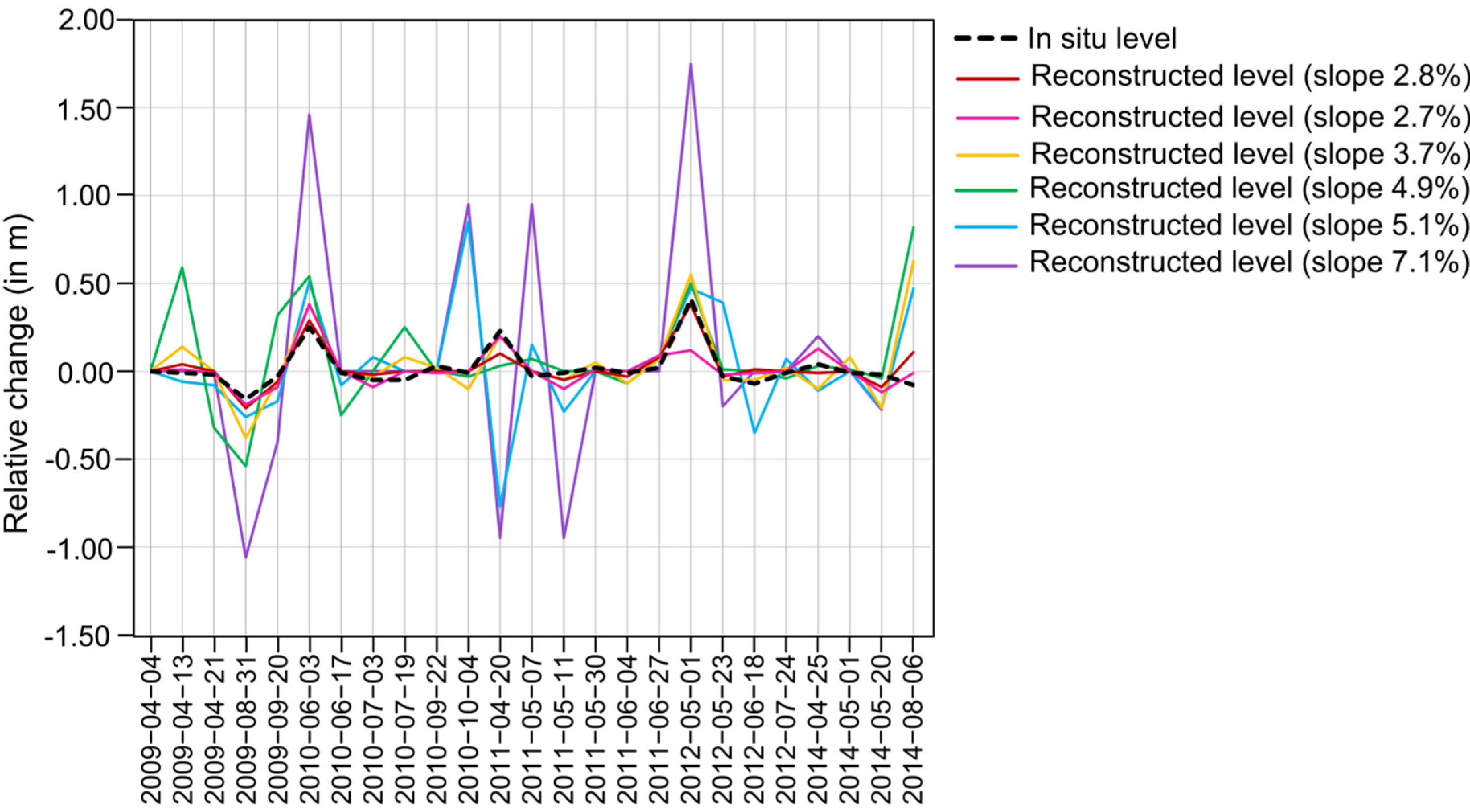
4.4. Lake Level Reconstruction


5. Discussion
- The water-land border needs to be delineated precisely. The automatic Otsu threshold on the NIR band showed the best results, but the approach is sensitive to shadows and thus to low solar angles. Dense vegetation cover hinders the accurate retrieval of water-land borders.
- The topographic data needs to be accurate as the lake level reconstruction is only as good as the underlying DEM. This is specifically true for the underwater surface model, which is not of very high quality due to sparse bathymetric point measurements. Due to the different quality levels of the DEM, the accuracy of lake level reconstruction depends here also on the lake level itself.
- The shoreline subset that is used for the retrieval of the lake level needs to be very shallow, so that the shift of the water-land border with changing lake level is maximized. Using RapidEye images, a decimeter accuracy of lake level reconstruction is only feasible if the shoreline slope is less than 3%.
6. Conclusions
Supplementary Materials
Acknowledgments
Author Contributions
Conflicts of Interest
References
- Kaiser, K.; Friedrich, J.; Oldorff, S.; Germer, S.; Mauersberger, R.; Natkhin, M.; Hupfer, M.; Pingel, A.; Schönfelder, J.; Spicher, V.; et al. Aktuelle hydrologische Veränderungen von Seen in Nordostdeutschland: Wasserspiegeltrends, ökologische Konsequenzen, Handlungsmöglichkeiten. In Wasserbezogene Anpassungsmaßnahmen an den Landschafts- und Klimawandel; Grünewald, U., Bens, O., Fischer, H., Hüttl, R.F., Kaiser, K., Eds.; Schweizerbart Science Publishers: Stuttgart, Germany, 2012; pp. 148–170. [Google Scholar]
- Mauersberger, R. Klassifikation der Seen für die Naturraumerkundung des nordostdeutschen Tieflandes. Arch. Naturschutz Landschaftsforsch. 2006, 3, 51–90. [Google Scholar]
- Germer, S.; Kaiser, K.; Bens, O.; Hüttl, R.F. Water Balance Changes and Responses of Ecosystems and Society in the Berlin-Brandenburg Region—A Review. DIE ERDE J. Geogr. Soc. Berlin 2011, 142, 65–95. [Google Scholar]
- Kaiser, K.; Koch, P.J.; Mauersberger, R.; Stüve, P.; Dreibrodt, J.; Bens, O. Detection and attribution of lake-level dynamics in north-eastern central Europe in recent decades. Reg. Environ. Chang. 2014, 14, 1587–1600. [Google Scholar] [CrossRef]
- Heine, I.; Francke, T.; Rogass, C.; Medeiros, P.H.A.; Bronstert, A.; Foerster, S. Monitoring Seasonal Changes in the Water Surface Areas of Reservoirs Using TerraSAR-X Time Series Data in Semiarid Northeastern Brazil. J. Sel. Top. Appl. Earth Obs. Remote Sens. 2014, 7, 3190–3199. [Google Scholar] [CrossRef]
- Van de Weyer, K.; Päzolt, J.; Tigges, P.; Raape, C.; Oldorff, S. Flächenbilanzierungen submerser Pflanzenbestände—Dargestellt am Beispiel des Großen Stechlinsees (Brandenburg) im Zeitraum von 1962–2008. Naturschutz Landschaftspfl. Brand. 2009, 18, 1–16. [Google Scholar]
- Brauns, M.; Garcia, X.F.; Pusch, M.T. Potential effects of water-level fluctuations on littoral invertebrates in lowland lakes. Hydrobiologia 2008, 613, 5–12. [Google Scholar] [CrossRef]
- Landesamt Brandenburg. Ökologische Charakterisierung der wichtigsten Brutgebiete für Wasservögel in Brandenburg. Stud. Tagungsberichte 2008, 57, 1–181. [Google Scholar]
- Landesamt Brandenburg (Ed.) Leitfaden zur Renaturierung von Feuchtgebieten in Brandenburg. Studien und Tagungsberichte des Landesumweltamtes, 2004; No. 50. Available online: http://www.lugv.brandenburg.de/cms/media.php/lbm1.a.3310.de/lua_bd50.pdf (accessed on 29 July 2015).
- Schmieder, K.; Dienst, M.; Ostendorp, W.; Joehnk, K. Effects of water level variations on the dynamics of the reed belts of Lake Constance. Ecohydrol. Hydrobiol. 2004, 4, 469–480. [Google Scholar]
- Hilt, S.; Henschke, I.; Rücker, J.; Nixdorf, B. Can submerged macrophytes influence turbidity and trophic state in deep lakes? Suggestions from a case study. J. Environ. Qual. 2010, 39, 725–733. [Google Scholar] [CrossRef] [PubMed]
- Hupfer, M.; Nixdorf, B. Zustand und Entwicklung von Seen in Berlin und Brandenburg. Materialien der Interdisziplinären Arbeitsgruppen (IAG Globaler Wandel—Regionale Entwicklung); Berlin-Brandenburgische Akademie der Wissenschaften: Leipzig, Germany, 2011; Diskussionspapier, No. 11. [Google Scholar]
- Ulrich, K.U. Vergleichende Untersuchungen zur Auswirkungen des Sediments auf die Wasserbeschaffenheit in Trinkwassertalsperren unter Berücksichtigung von Stauspiegelschwankungen; Cuvillier Verlag: Göttingen, Germany, 1998. [Google Scholar]
- Verpoorter, C.; Kutser, T.; Tranvik, L. Automated mapping of water bodies using Landsat multispectral data. Limnol. Oceanogr. Methods 2012, 10, 1037–1050. [Google Scholar] [CrossRef]
- Muster, S.; Heim, B.; Abnizova, A.; Boike, J. Water Body Distributions Across Scales: A Remote Sensing Based Comparison of Three Arctic TundraWetlands. Remote Sens. 2013, 5, 1498–1523. [Google Scholar] [CrossRef] [Green Version]
- Maillard, P.; Pivari, M.O.; Luis, C.H.P. Remote Sensing for Mapping and Monitoring Wetlands and Small Lakes in Southeast Brazil. In Remote Sensing of Planet Earth; Chemin, Y., Ed.; InTech: Rijeka, Croatia, 2012; pp. 23–46. [Google Scholar]
- Wang, J.; Sheng, Y.; Tong, T.S.D. Monitoring decadal lake dynamics across the Yangtze Basin downstream of Three Gorges Dam. Remote Sens. Environ. 2014, 152, 251–269. [Google Scholar] [CrossRef]
- Alesheikh, A.; Ghorbanali, A.; Nouri, N. Coastline change detection using remote sensing. Int. J. Environ. Sci. Technol. 2007, 4, 61–66. [Google Scholar] [CrossRef]
- White, K.; El Asmar, H.M. Monitoring changing position of coastlines using Thematic Mapper imagery, an example from the Nile Delta. Geomorphology 1999, 29, 93–105. [Google Scholar] [CrossRef]
- Lipakis, M.; Chrysoulakis, N. Shoreline extraction using satellite imagery. In Beach Erosion Monitoring: Results from BEACHMED-e/OpTIMAL Project; Pranzini, E., Wetzel, L., Eds.; Nuova Grafica Fiorentina: Florence, Italy, 2008; pp. 81–96. [Google Scholar]
- Li, X.; Damen, M.C.J. Coastline change detection with satellite remote sensing for environmental management of the Pearl River Estuary, China. J. Mar. Syst. 2010, 82, S54–S61. [Google Scholar] [CrossRef]
- Gens, R. Remote sensing of coastlines: Detection, extraction and monitoring. Int. J. Remote Sens. 2010, 31, 1819–1836. [Google Scholar] [CrossRef]
- Pardo-Pascual, J.E.; Almonacid-Caballer, J.; Ruiz, L.A.; Palomar-Vázquez, J. Automatic extraction of shorelines from Landsat TM and ETM+ multi-temporal images with subpixel precision. Remote Sens. Environ. 2012, 123, 1–11. [Google Scholar] [CrossRef]
- Baup, F.; Frappart, F.; Maubant, J. Combining high-resolution satellite images and altimetry to estimate the volume of small lakes. Hydrol. Earth Syst. Sci. 2014, 18, 2007–2020. [Google Scholar] [CrossRef]
- Maillard, P.; Bercher, N.; Calmant, S. New processing approaches on the retrieval of water levels in Envisat and SARAL radar altimetry over rivers: A case study of the São Francisco River, Brazil. Remote Sens. Environ. 2015, 156, 226–241. [Google Scholar] [CrossRef]
- Abarca-Del-Rio, R.; CrÉtaux, J.F.; Berge-Nguyen, M.; Maisongrande, P. Does Lake Titicaca still control the Lake Poopó system water levels? An investigation using satellite altimetry and MODIS data (2000–2009). Remote Sens. Lett. 2012, 3, 707–714. [Google Scholar] [CrossRef]
- Da Silva, J.S.; Seyler, F.; Calmant, S.; Rotunno Filho, O.C.; Roux, E.; Araújo, A.A.M.; Guyot, J.L. Water level dynamics of Amazon wetlands at the watershed scale by satellite altimetry. Int. J. Remote Sens. 2012, 33, 3323–3353. [Google Scholar] [CrossRef]
- Gupta, R.; Banerji, S. Monitoring of reservoir volume using LANDSAT data. J. Hydrol. 1985, 77, 159–170. [Google Scholar] [CrossRef]
- Smith, L.C. Satellite remote sensing of river inundation area, stage, and discharge: A review. Hydrol. Process. 1997, 11, 1427–1439. [Google Scholar] [CrossRef]
- Brakenridge, G.R.; Nghiem, S.V.; Anderson, E.; Chien, S. Space-based measurement of river runoff. Eos Trans. Am. Geophys. Union 2005, 86, 185. [Google Scholar] [CrossRef]
- Alsdorf, D.E.; Rodriguez, E.; Lettenmaier, D.P. Measuring surface water from space. Rev. Geophys. 2007, 45, 1–24. [Google Scholar] [CrossRef]
- Hostache, R.; Matgen, P.; Schumann, G.; Member, S.; Puech, C.; Hoffmann, L.; Pfister, L. Model Calibration Uncertainties Using Satellite SAR Images of Floods. Trans. Geosci. Remote Sens. 2009, 47, 431–441. [Google Scholar]
- Kaiser, K.; Heinrich, I.; Heine, I.; Natkhin, M.; Dannowski, R.; Lischeid, G.; Schneider, T.; Henkel, J.; Küster, M.; Heussner, K.; et al. Multi-decadal lake-level dynamics in north-eastern Germany as derived by a combination of gauging, proxy-data and modelling. J. Hydrol. 2015, in press. [Google Scholar] [CrossRef]
- Germer, S.; Kaiser, K.; Mauersberger, R. Sinkende Seespiegel in Nordostdeutschland: Vielzahl hydrologischer Spezialfälle oder Gruppen von Ähnlichen Seesystemen? In Aktuelle Probleme im Wasserhaushalt von Nordostdeutschland: Trends, Ursachen, Lösungen; Scientific Technical Report 10/10; Deutsches GeoForschungsZentrum: Potsdam, Germany, 2010. [Google Scholar]
- Data from Deutscher Wetterdienst. Available online: http://www.dwd.de/ (accessed on 10 March 2015).
- Landesamt für Umwelt Naturschutz und Geologie Mecklenburg-Vorpommern. Gutachtlicher Landschaftsrahmenplan Mecklenburgische Seenplatte. 2011. Available online: http://www.lung.mv-regierung.de/dateien/glrp_ms_06_2011.pdf (accessed on 29 July 2015).
- Ministerium für Landwirtschaft, Umwelt und Verbraucherschutz Mecklenburg-Vorpommern. Available online: http://www.regierung-mv.de/cms2/Regierungsportal_prod/Regierungsportal/de/lm/index.jsp (accessed on 4 December 2014).
- Staatliches Amt für Landwirtschaft und Umwelt Mecklenburgische Seenplatte (MS). Available online: http://www.stalu-mv.de/cms2/StALU_prod/StALU/de/ms/index.jsp (accessed on 8 January 2015).
- Sandau, R. Status and trends of small satellite missions for Earth observation. Acta Astronaut. 2010, 66, 1–12. [Google Scholar] [CrossRef]
- Landesamt für innere Verwaltung Mecklenburg Vorpommern. Available online: http://www.laiv-mv.de/land-mv/LAiV_prod/LAiV/AfGVK/index.jsp (accessed on 3 May 2013).
- RapidEye—Satellite Imagery Product Specifications, Version 6.1, April 2015. Available online: http://blackbridge.com/rapideye/upload/RE_Product_Specifications_ENG.pdf (accessed on 27 July 2015).
- Behling, R.; Roessner, S.; Segl, K.; Kleinschmit, B.; Kaufmann, H. Robust automated image co-registration of optical multi-sensor time series data: Database generation for multi-temporal landslide detection. Remote Sens. 2014, 6, 2572–2600. [Google Scholar] [CrossRef]
- Amt für Geoinformation, V.K. Satellitenpositionierungsdienst-SAPOS®. Available online: http://www.laiv-mv.de/land-mv/LAiV_prod/LAiV/AfGVK/Festpunkte,_SAPOS/SAPOS/index.jsp (accessed on 27 July 2015).
- Arbor, A.; Gilmer, D.S.; Fish, U.S.; Service, W. Utilization of Satellite Data for Inventorying Prairie Ponds and Lakes. Photogramm. Eng. Remote Sens. 1976, 42, 685–694. [Google Scholar]
- Kropáček, J.; Braun, A.; Kang, S.; Feng, C.; Ye, Q.; Hochschild, V. Analysis of lake level changes in Nam Co in central Tibet utilizing synergistic satellite altimetry and optical imagery. Int. J. Appl. Earth Obs. Geoinf. 2012, 17, 3–11. [Google Scholar] [CrossRef]
- Roessler, S.; Wolf, P.; Schneider, T. Multispectral Remote Sensing of Invasive Aquatic Plants Using RapidEye. In Earth Observation of Global Changes (EOGC); Krisp, J.M., Meng, L., Pail, R., Stilla, U., Eds.; Lecture Notes in Geoinformation and Cartography; Springer: Berlin, Germany, 2013; pp. 109–123. [Google Scholar]
- Ji, L.; Zhang, L.; Wylie, B. Analysis of Dynamic Thresholds for the Normalized Difference Water Index. Photogramm. Eng. Remote Sens. 2009, 75, 1307–1317. [Google Scholar] [CrossRef]
- Lu, S.; Ouyang, N.; Wu, B.; Wei, Y.; Tesemma, Z. Lake water volume calculation with time series remote-sensing images. Int. J. Remote Sens. 2013, 34, 7962–7973. [Google Scholar] [CrossRef]
- Li, W.; Du, Z.; Ling, F.; Zhou, D.; Wang, H.; Gui, Y.; Sun, B.; Zhang, X. A Comparison of Land Surface Water Mapping Using the Normalized Difference Water Index from TM, ETM+ and ALI. Remote Sens. 2013, 5, 5530–5549. [Google Scholar] [CrossRef]
- McFeeters, S.K. The use of the Normalized Difference Water Index (NDWI) in the delineation of open water features. Int. J. Remote Sens. 1996, 17, 1425–1432. [Google Scholar] [CrossRef]
- Lu, S.; Wu, B.; Yan, N.; Wang, H. Water body mapping method with HJ-1A/B satellite imagery. Int. J. Appl. Earth Obs. Geoinf. 2011, 13, 428–434. [Google Scholar] [CrossRef]
- Otsu, N. A threshold selection method from Gray-level. IEEE Trans. Syst. Man Cybern. 1979, 9, 62–66. [Google Scholar]
- Puech, C.; Raclot, D. Using geographical information systems and aerial photographs to determine water levels during floods. Hydrol. Process. 2002, 16, 1593–1602. [Google Scholar] [CrossRef]
- Hostache, R.; Matgen, P.; Schumann, G.; Puech, C.; Hoffmann, L.; Pfiste, L. Water level estimation and reduction of hydraulic model calibration uncertainties using satellite SAR images of floods. Trans. Geosci. Remote Sens. 2009, 47, 431–441. [Google Scholar] [CrossRef]
- Bochow, M.; Heim, B.; Küster, T.; Rogaß, C.; Bartsch, I.; Segl, K.; Reigber, S.; Kaufmann, H. On the Use of Airborne Imaging Spectroscopy Data for the Automatic Detection and Delineation of Surface Water Bodies. In Remote Sensing of Planet Earth; Chemin, Y., Ed.; InTech: Rijeka, Croatia, 2012; pp. 3–22. [Google Scholar]
- Lira, J. Segmentation and morphology of open water bodies from multispectral images. Int. J. Remote Sens. 2006, 27, 4015–4038. [Google Scholar] [CrossRef]
- Qiao, C.; Luo, J.; Sheng, Y.; Shen, Z.; Zhu, Z.; Ming, D. An Adaptive Water Extraction Method from Remote Sensing Image Based on NDWI. J. Indian Soc. Remote Sens. 2012, 40, 421–433. [Google Scholar] [CrossRef]
- Davaasuren, N.; Meesters, H.W.G. Extent and Health of Mangroves Mangroves in Lac Bay Bonaire Using Satellite Data; IMARES Wageningen UR: Haringkade, The Netherland, 2012. [Google Scholar]
- Päzolt, J.; Landesamt für Umwelt, Gesundheit und Verbraucherschutz, Brandenburg, Germany. Personal Communication, 2015.
- Mathes, J.; Ministerium für Landwirtschaft, Umwelt und Geologie, Mecklenburg-Vorpommers, Germany. Personal Communication, 2015.
- Lillesand, T.M.; Kiefer, R.W.; Chipman, J.W. Remote Sensing and Image Interpretation, 6th ed.; Wiley: Hoboken, NJ, USA, 2008. [Google Scholar]
© 2015 by the authors; licensee MDPI, Basel, Switzerland. This article is an open access article distributed under the terms and conditions of the Creative Commons Attribution license (http://creativecommons.org/licenses/by/4.0/).
Share and Cite
Heine, I.; Stüve, P.; Kleinschmit, B.; Itzerott, S. Reconstruction of Lake Level Changes of Groundwater-Fed Lakes in Northeastern Germany Using RapidEye Time Series. Water 2015, 7, 4175-4199. https://doi.org/10.3390/w7084175
Heine I, Stüve P, Kleinschmit B, Itzerott S. Reconstruction of Lake Level Changes of Groundwater-Fed Lakes in Northeastern Germany Using RapidEye Time Series. Water. 2015; 7(8):4175-4199. https://doi.org/10.3390/w7084175
Chicago/Turabian StyleHeine, Iris, Peter Stüve, Birgit Kleinschmit, and Sibylle Itzerott. 2015. "Reconstruction of Lake Level Changes of Groundwater-Fed Lakes in Northeastern Germany Using RapidEye Time Series" Water 7, no. 8: 4175-4199. https://doi.org/10.3390/w7084175