Integrating Ecosystem Services and Health into Landscape Functional Zoning: A Case Study of the Jinan Southern Mountainous Area, China

Abstract

Ecosystems and their services to society have exhibited dramatic degradation all over the world, and landscape planning based on ecosystem service (ES) science is a promising way to mitigate ES loss and improve human well-being. However, ecosystem health, which is crucial for intrinsic ecosystem values, may be overlooked in ES-based landscape planning. Therefore, we proposed a landscape functional zoning method by combining the ES and EH using the Jinan Southern Mountainous Area as a case study. Specifically, we first quantified and mapped six ESs (including regulating, cultural, and provisioning services) and three EH properties (ecosystem vigor, organization, and resilience). Then, we used coupling coordination analysis to determine the coordination of the ES and EH, and adopted bundle analysis to reveal ES-EH compositions. Finally, landscape functional zones were delineated by spatially overlapping the maps of ES-EH bundle types and coupling coordination degrees. The results show that the different ESs and EH properties exhibited uneven spatial distributions. In terms of the ES-EH coupling coordination degree, high values were located along the mountains and aggregated in the eastern part of the study area, and the Caishi town had the highest coupling coordination degree on the town scale. Furthermore, five ES-EH bundle types were identified, i.e., bundles of multifunctionality, subordinate multifunctionality, the highest crop production, ESs and EH properties of medium levels, and ESs and EH properties of low levels. Finally, nine landscape functional zones based on the ES-EH bundle and coupling coordination were identified, and the grids within one zone were homogeneous in terms of their ES-EH compositions and coupling coordination. This study can contribute to the integration of ES and EH into landscape planning and provides a zoning method as a spatial instrument to achieve synergic ES-EH management.

1. Introduction

In the context of global climate change and increasingly intensive human activities, ecosystems and their contributions to society have shown dramatic degradation [1]. Such degradation has threatened human well-being from different aspects, such as basic material [2], security [3], and mental and physical health [4]. Managing ecosystems for sustainable development has become one of the most crucial issues for scientists and decision-makers [5]. The concept of ecosystem service (ES) has been proposed to link ecosystems and socioeconomic systems [6]. The ES classification provides a systematic inventory of benefits provided by ecosystems for people [7], and ES quantification and mapping provide spatially explicit information for ES-related decision making [8]. In recent years, the ES concept has been widely integrated into landscape planning, e.g., urban green infrastructure [9], conservation planning [10], and controlling urban expansion [11]. Landscape planning has acted as one of the most important ES science–policy interfaces [12].

Spatial zoning has been considered an important part of the design stage of landscape planning [13]. Landscapes normally show great spatial heterogeneity in terms of the ecosystem structure and process, and thus decision-makers have to consider how to manage different areas of a complex landscape [14]. The zoning scheme can simplify chaotic information by dividing landscapes into several distinct zones, and areas in each zone remain homogeneous in terms of the landscape structure and function [15]. Therefore, zoning can make management strategies fit specific socio-ecological conditions of different zones [16]. Zone identification based on ES information is normally regarded as landscape functional zoning, which has been widely used to guide landscape planning [17]. For example, previous studies have developed different zoning schemes on multiple scales, e.g., the urban agglomeration [16], prefecture [18], and watershed [19]. It has been shown that landscape functional zoning has great potential to identify specific ecological risks [20], improve conservation efficiency [21] and mitigate conflicts between ecological restoration and socioeconomic development [15]. However, zoning solely relying on ESs may overlook some important landscape characteristics that are not directly related to human well-being but are crucial for maintaining ecosystem integrity.

Ecosystem health (EH) refers to the ability of ecosystems to maintain self-regulation and recovery [22], and is fundamental to many ecological processes and functions, such as energy capture, nutrient cycling, and species migration [23]. Moreover, EH plays an important role in mitigating anthropogenic pressures on ecosystems [24]. Compared with the ES concept, EH emphasizes natural ecosystems themselves, and has drawn the increasing attention of scientists and decision-makers to landscape features essential for healthy ecosystems [25] The anthropocentric value of the ES has been criticized by some ecologists, as decision making solely based on ESs may degrade the intrinsic value of ecosystems [26]. Scientists have gradually realized that linking EH and ES together to landscape functional zoning can mitigate such a defect, and have developed several landscape assessment frameworks combining ESs and EH. For example, Zhao and Huang [27] have developed a combined index of ESs and EH to evaluate the landscape sustainability level and identified conservation priority with the support of this index. Qiao and Huang [23] constructed an improved EH evaluation framework which not only includes EF properties but also the ES value. Despite those efforts, rare studies have formulated landscape zoning based on the combination of ESs and EH. Such a zoning may provide a novel spatial tool to protect ecosystems’ ability to satisfy human demands and maintain sustainable ecosystems.

The ability of ecosystems to provide multiple ESs normally acts as the proxy of the overall ecosystem performance [7]. The landscape functional zones can be delineated according to the range of the ecosystem performance, and then planners can determine the management intensity [28]. However, how to evaluate the overall ecosystem performance from an ES-EH coupled perspective still needs to be addressed. Coupling coordination analysis provides a novel perspective to portray the overall coordination between the ES and EH. The concept of coupling coordination origins from the field of physics, and refers to the desired state where different subsystems are interactive and support each other [29]. Coupling coordination not only represents the overall high quality of subsystems, but is also involved with the positive relationship between different subsystems [30]. Coupling coordination has great potential to support the decision making of ecosystem management [29]. Therefore, taking the ES and EH as subsystems and analyzing their coupling coordination can reveal the overall ability of ecosystems to provide ESs and maintain the EH status, and subsequently is suitable to be used in landscape functional zoning.

Another promising perspective for landscape functional zoning is the ES bundle analysis. An ES bundle refers to a series of ESs co-occurring repeatedly among landscapes, and has been used to illustrate the ES composition [31]. The difference in the ES composition is minimized within one bundle and maximized between different bundles [15]. Planners tend to identify landscape functional zones according to the ES composition represented by the ES bundle, and can formulate targeted planning strategies to manage multiple ESs together instead of one single ES [19]. Successful cases of landscape functional zoning based on the ES bundle have been shown in previous studies, which are on the scales of the watershed [32], urban agglomeration [15], and nation [33]. However, few studies have bundled ES and EH properties together to delineate landscape functional zones, which hinders the simultaneous management of ES and EH. Bundling ES and EH properties for zoning can prevent unexpected decreases in some EH properties induced by maximizing the provision of specific ESs.

To narrow the research gaps mentioned above, we aimed to propose a landscape functional zoning method based on the ES and EH, and used the Jinan Southern Mountainous Area (JSMA) as a case study. The objectives of this study are as follows: (1) revealing ES-EH bundles and their spatial patterns; (2) analyzing ES-EH coupling coordination and its spatial pattern; and (3) proposing the landscape functional zoning method based on the combination of ES-EH bundles and coupling coordination. This study provides a novel spatial tool for the synergetic management of the ES and EH, which can contribute to maintaining human well-being and sustainable ecosystems.

2. Study Area

The JSMA (116°41′15″ E~117°18′45″ E, 36°12′30″ E~36°42′15″ E) is located in the southeastern part of the Jinan Prefecture and involves 16 towns/counties, while the total area of the JSMA is 837 km². JSMA has complex geomorphic features, where a variety of landforms are distributed, such as low mountains, middle mountains, hills, intermountain platforms, and intermountain basins [34]. The study area is situated in the warm temperate continental monsoon climate zone, and has an annual average temperature of 13.7 °C and average precipitation of 644.4 mm. The elevation ranges from 30 m to 896 m, and the elevation in the eastern part is higher than that in the western part. In 2020, farmland was the land use type with the biggest area proportion of the JSMA (38.09%), while forestland, grassland, and built-up land accounted for 36.72%, 16.95%, and 5.85%, respectively (Figure 1). Platycladus orientalis Linn and Populus tomentosa Carrière are the dominant tree species, while the main meadow types include Arthraxon hispidus Thunb, and Deyeuxia arundinacea Linnaeus. Wheat is the main crop type in the study area, and wheat production is important for the crop demand of the whole Jinan Prefecture. Due to abundant natural ecosystems, JSMA acts as an important ES-providing area. However, in past decades, farmland and built-up land have expanded greatly at the cost of natural ecosystems. Furthermore, the JSMA has continuously developed secondary and tertiary industries since the 1990s, e.g., mining, real estate, and machine manufacturing, which exerts severe pressure on local ecosystems. Therefore, landscape planning with a scientific basis is urgently needed to manage the ESs and EH of the JSMA.

3. Methodology

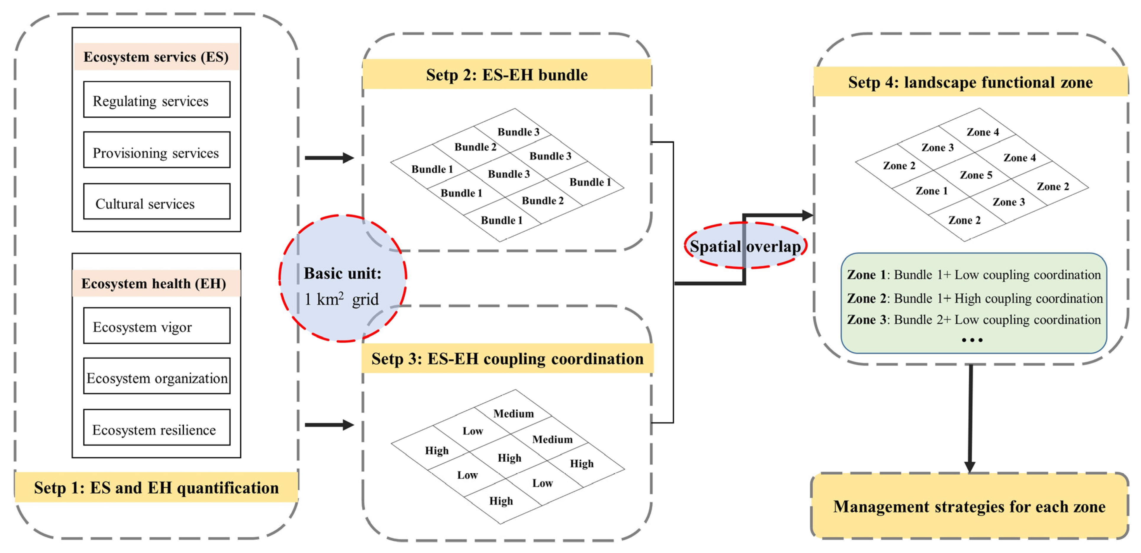
3.1. Research Design

The year 2020 was taken as the study period, and we selected the 1 km² grid as the basic unit due to the fact that (1) this unit has been widely used in previous studies related to ESs and EH [35]; (2) this unit is small compared with the study area, and can serve landscape planning; (3) several ESs and EH properties have to be calculated on the scale of the grid compose of various land use/cover types. This study was processed with four steps (Figure 2). In the first step, we quantified different ESs (including regulating, cultural, and provisioning service classes) and EH properties (ecosystem vigor, organization, and resilience), which were the basis of the next three steps. The second step is to evaluate ES-EH coupling coordination, which was used to reveal the overall performance of ecosystems in terms of satisfying human demands and maintaining intrinsic ecosystem values. The third step is ES-EH bundle identification, which was used to determine ES-EH compositions and their spatial patterns. In the last step, we overlapped the maps of ES-EH bundle types and coupling coordination classes, and the grids sharing a similar bundle type and coupling coordination class were regarded as individual management zones. For each zone, the ES-EH coupling coordination degree indicates the conservation intensity, while the ES-EH bundle can illustrate the types of ESs and EH properties that should be conservation targets. Based on the conservation intensity and the target in each zone, specific management strategies for each landscape functional zone were proposed.

3.2. Data Source

In this study, we used multisource data to quantify different ESs and EH properties, mainly including land use/cover data, meteorological data, soil characteristics, topography data, and so on (

Table 1. The data information and source.

Data	Time	Resolution	Source
Landsat 8 remote sensing image (path/row: 122/34 and 122/35)	July–September, 2020	30 m	Chinese geospatial data cloud (http://www.gscloud.cn, 31 August 2024)
GlobeLand30 land use/cover data	2020	30 m	http://www.globallandcover.com, 31 August 2024
Annually average temperature	2020	1 km	National Earth System Science Data center (http://www.geodata.cn, 31 August 2024)
Annual precipitation	2020	1 km	National Earth System Science Data center (http://www.geodata.cn, 31 August 2024)
Potential evapotranspiration	2020	1 km	National Earth System Science Data center (http://www.geodata.cn, 31 August 2024)
Digital elevation model (ASTER GDEM)	2009	30 m	Chinese geospatial data cloud (http://www.gscloud.cn, 31 August 2024)
Harmonized World Soil Database	2009	1 km	Food and Agriculture Organization of the United Nations (https://www.fao.org/soils-portal/, 31 August 2024)
Transportation network	2020	Vector	National Geomatics Center of China (http://www.ngcc.cn, 31 August 2024)
Administrative boundary	2020	Vector	National Geomatics Center of China (http://www.ngcc.cn, 31 August 2024)
Statistics data (annual crop yield and water resources)	2020	Numerical value (county level)	Shandong Provincial Bureau of statistics (http://tjj.shandong.gov.cn, 31 August 2024)

). Most data are for the year 2020 except those insensitive to temporal changes.

3.3. ES Selection and Quantification

According to the ES classification framework, we selected different ESs belonging to all the ES classes, i.e., regulating, provisioning, and cultural services [36]. Each ES selected should be crucial to local human well-being and socioeconomic development. Additionally, we preferentially selected the ESs that have been listed as management goals in environmental management and spatial planning policies in the JSMA. In this study, we determined six types of ESs, including water retention, carbon storage, soil retention, water purification, natural aesthetics and recreation, and crop production. The JSMA is the main water resource conservation area of the Jinan Prefecture, so water retention is one focus of local ES management [37]. Carbon storage plays an important role in climate change mitigation, while soil conservation was selected due to the high soil erosion vulnerability in the study area [34]. Farmland is a major land use type in the study area, representing a high water pollution risk. Therefore, water purification should be managed to mitigate non-point source pollution. The JSMA owns great tourism resources that contribute to human mental health and residents’ income, so natural aesthetics and recreation is one ES that needs to be integrated into landscape planning [38]. Agriculture is one of the main production activities that local residents work in; thus, crop production was also evaluated in this study. All the ESs selected have been regarded as the ecological conservation targets in official planning policies, including the Plan for Coordinating Development and Conservation in the JSMA (http://www.jinan.gov.cn/, accessed on 31 August 2024), Combined Master Plan in the JSMA from 2017 to 2035 (http://jnns.jinan.gov.cn/, accessed on 31 August 2024), and Territory Space Plan in the JSMA from 2022 to 2035 (http://jnns.jinan.gov.cn/, accessed on 31 August 2024). In addition, to ensure ES evaluation accuracy, the values of the parameters for ES quantification were obtained from the previous studies in regions with similar ecological conditions to those of the JSMA. Specific parameter settings for ES quantification can be seen in the electronic Supplementary Materials (ESM).

3.3.1. Water Retention

Water retention can be understood as ecosystems’ ability to retain and conserve water from rainfall, contributing to vegetation growth and runoff reduction [28]. In this study, we quantified water retention on the pixel scale with three steps: (1) quantifying annual water yield with the Water Yield Module of InVEST version 3.13.0; (2) quantifying surface runoff based on the runoff coefficient and precipitation; and (3) calculating water retention by subtracting surface runoff from water yield for each pixel. The Water Yield Module of InVEST is designed based on the water balance equation, and suggests that water yield is equal to the difference between precipitation and evapotranspiration [39] Thereafter, the runoff coefficient is the proportion of surface runoff in total precipitation, which can be determined by land use/cover types (the coefficient can be seen in the previous study of Li et al. [28]). Then, we subtracted surface runoff from water yield to calculate water retention for each pixel (Equation (2)).

$${WY}_k=(1-{\displaystyle \frac{{AET}_k}{P_k}})\times P_k$$

(1)

where ${WY}_k$ is water yield in pixel $k$ (mm); ${AET}_j$ and $P_j$ represent the actual evapotranspiration and precipitation of pixel $k$ (mm), respectively. In the Water Yield Module, actual evapotranspiration is calculated with the reference evapotranspiration, root depth, soil property, and vegetation available water content. More explicit explanations and equations of actual evapotranspiration can be found in the InVEST Users’ Guide [39].

$${WR}_k={WY}_k-P_k\times {RC}_k$$

(2)

where ${WR}_k$ is water retention of pixel $k$ (mm); ${RC}_k$ is the runoff coefficient of pixel $k$ (dimensionless). The parameters can be seen in Tables S1 and S2 of the ESM.

3.3.2. Carbon Storage

We adopted the Carbon Storage Module of the InVEST Model for carbon storage quantification. This module assumes that carbon storage can be calculated by accumulating the carbon stocks of four carbon pools (aboveground biomass, underground biomass, soil carbon, and dead organic matter pools), and the carbon stocks per unit area of four carbon pools are determined by land use/cover types [39]. In this study, parameters of carbon density for each land use/cover type were obtained from previous studies in the study area and its adjacent areas [40]. The equation is as follows:

$$CS={CS}_{above}+{CS}_{under}+{CS}_{soil}+{CS}_{dead}$$

(3)

where $CS$ is the carbon storage (t/hm²); ${CS}_{above}$, ${CS}_{under}$, ${CS}_{soil}$, and ${CS}_{dead}$ represent carbon stocks per hectare of aboveground biomass, underground biomass, soil carbon, and dead organic matter pools, respectively (t/hm²). The specific parameters can be seen in Table S3 of the ESM.

3.3.3. Soil Conservation

Soil conservation is defined as the capacity of ecosystems to prevent soil erosion, and was calculated with the Revised Universal Soil Loss Equation (RUSLE) in this study. RUSLE considers the influences of rainfall, soil properties, topography, and human management on actual and potential soil erosion to quantify soil conservation [41]. In this model, soil erosion in the current situation of the land use/cover pattern is entitled actual soil erosion, while potential soil erosion refers to soil erosion in an assumed situation where all the lands are covered by bare land without any soil erosion management [42]. Soil conservation is the difference between actual and potential soil erosion, and the equation is expressed as follows:

$$SC={SE}_{Potential}-{SE}_{actual}=(1-C\times P)\times R\times K\times LS$$

(4)

where $SC$, ${SE}_{Potential}$, and ${SE}_{Actual}$ (t/hm²) stand for soil conservation, potential, and actual soil erosion, respectively; R represents the rainfall erosivity factor (MJ·mm·hm⁻²·h⁻¹), and K denotes the soil erodibility factor (t·h·MJ⁻¹·mm⁻¹); $LS$, $C$, and $P$ are dimensionless parameters, and represent the slope length and steepness factor, vegetation coverage factor, and soil erosion management factor, respectively.

3.3.4. Water Purification

We used the nitrogen export as the water purification proxy, and quantified the nitrogen export on the pixel scale with the Nutrient Delivery Ratio (NDR) Module of the InVEST Model. The lower the nitrogen export is, the higher the water purification is [43]. This module can simulate where the nitrogen load is distributed in landscapes and how the nitrogen load is transported by the runoff. The nitrogen export is the part of the nitrogen load that is not retained by downstream ecosystems and flows into the stream. The nitrogen export for each pixel is determined by the nitrogen load, topography, downstream length, and nitrogen retention capacity provided by downstream ecosystems. The specific formulas and explicit explanations can be seen in the InVEST Users’ Guide (Sharp et al., 2014). For validation, the simulated water purification value was compared with the observed data. Since the observed data related to water purification is only available on the prefecture scale, the comparison was conducted on the scale of the Jinan Prefecture. The observed nitrogen export amount (1317.69 t) in the Jinan Prefecture was obtained from the Bulletin of Jinan Ecological Environment Bureau (http://jnepb.jinan.gov.cn/, 31 August 2024), while the nitrogen export calculated with the parameters used in this study was 1351.42 t. Such comparison indicated that the evaluation of this study is reliable.

3.3.5. Natural Aesthetics and Recreation

The visual quality index was used to quantify natural aesthetics and recreation in this study [44]. The visual quality index considers five indicators influencing natural recreation and aesthetics, including terrain, water scene, green space, naturalness, and accessibility, and is calculated by adding the normalized values of these five indicators (Cui et al., 2019 [45]):

$$\begin{gathered} {VQI}_{total}= {VQI}_{terrain}+{VQI}_{water scene}+{VQI}_{green space}+{VQI}_{naturalness} \\ +{VQI}_{accessibility} \end{gathered}$$

(5)

where ${VQI}_{total}$ is the visual quality index (dimensionless, 0~1), while ${VQI}_{terrain}$, ${VQI}_{water scene}$, ${VQI}_{green space}$, ${VQI}_{naturalness}$, and ${VQI}_{accessibility}$ stand for the normalized value of terrain, water scene, green space, naturalness, and accessibility, respectively (0~1); ${VQI}_{terrain}$ is reflected by the terrain roughness index [45]; ${VQI}_{water scene}$ and ${VQI}_{accessibility}$ are calculated with minimal distances to the waterbody and road, and the smaller minimal distance denotes the larger value of ${VQI}_{water scene}$ and ${VQI}_{accessibility}$; ${VQI}_{green space}$ takes the green space proportion as the proxy, while ${VQI}_{naturalness}$ adopts the inverse value of the built-up land proportion for the indicator.

3.3.6. Crop Production

We quantified crop production for each farmland pixel using the annual crop yield of the Jinan Prefecture (derived from local statistics data) and farmland NDVI. Since previous studies have shown that NDVI has been widely used as the proxy of crop production capacity [46], we used the farmland NDVI value to spatialize crop production of the prefecture scale:

$${CP}_k={\displaystyle \frac{{NDVI}_k}{{NDVI}_{mean}}}\times {CP}_{mean}$$

(6)

where ${CP}_k$ is the crop production capacity of farmland pixel $k$ (kg/hm²); ${NDVI}_i$ represents the NDVI value of farmland pixel $k$ (dimensionless), while ${NDVI}_{mean}$ is the mean farmland NDVI value in the Jinan Prefecture (dimensionless); ${CP}_{mean}$ is the annual average crop production per hectare of farmland in the Jinan Prefecture (kg/hm²).

3.4. EH Quantification

EH emphasizes the capacity of ecosystems to maintain their healthy statuses under human pressures, and is mainly involved with three aspects, i.e., ecosystem vigor, organization, and resilience [25]. Therefore, we used the ecosystem vigor–organization–resilience (VOR) model to quantify EH. This model is not only one of the most commonly used methods for EH evaluation, but also shows great feasibility in previous studies [22,23,47]. According to this model, EH is a combined result of ecosystem organization, vigor, and resilience. Ecosystem organization was calculated on the 1 km² grid scale, while ecosystem vigor and resilience were calculated for each pixel and then counted on the 1 km² grid scale.

3.4.1. Ecosystem Vigor

Ecosystem vigor denotes the metabolism and primary productivity of ecosystems [48]. In this study, NDVI was used as the proxy of ecosystem vigor, since NDVI can effectively represent the primary productivity and metabolism ratio [49]. The equation is expressed as follows [50]:

$$\mathrm{N}\mathrm{D}\mathrm{V}\mathrm{I}={\displaystyle \frac{\left({\rho }_{NIR}-{\rho }_{RED}\right)}{\left({\rho }_{NIR}+{\rho }_{RED}\right)}}$$

(7)

where ${\rho }_{RED}$ and ${\rho }_{NIR}$ are the red and near-infrared bands, which correspond to the fourth and fifth brand reflectivity in the Landsat 8 OLI/TIRS image.

3.4.2. Ecosystem Organization

Ecosystem organization represents the interaction between ecosystems and their structural stability, and is normally reflected by the landscape pattern metric on the landscape scale [24]. According to previous studies, we selected different landscape pattern metrics from three aspects of ecosystem vigor, i.e., connectivity for the whole landscape, connectivity for the green space, and landscape heterogeneity [48]. All the landscape metrics have clear planning implications and have been widely used in ecosystem organization evaluation [47,51]. The Landscape Contagion Index and Division Index analyzed on the landscape scale were adopted to denote landscape connectivity from the aspects of patch contagion and spatial adjacency. In terms of green space connectivity, due to the inapplicability of the Landscape Contagion Index on the class level, this metric was replaced by another commonly used metric of Cohesion Index. Therefore, the Cohesion Index and Division Index on the class level were used to represent green space connectivity. Moreover, the Mean Fractal Dimension Index and Shannon Evenness Index were used to indicate landscape heterogeneity in terms of shape and composition. Finally, we used the weighted summation method to calculate the overall level of ecosystem organization (the weight for each metric is derived from previous studies of [22,47,48]:

$$\begin{array}{cc}\hfill EO=0.35\times LC& +0.3\times GS+0.35\times LH\hfill \\ & =\left(0.2\times LCI+0.15\times {DI}_l\right)+\left(0.2\times CI+0.1\times {DI}_{gs}\right)\hfill \\ & +\left(0.25\times SHEI+0.1\times MWFD\right)\hfill \end{array}$$

(8)

where $EO$ denotes ecosystem organization, while $\mathrm{C}L$, $\mathrm{C}GS$, and $LH$ refer to the connectivity for landscape, the connectivity for green space, and landscape heterogeneity, respectively; $LCI$ and ${DI}_l$ stand for Landscape Contagion Index and Division Index (on the landscape scale), respectively; $CI$ and ${DI}_{gs}$ refer to the Cohesion Index and Division Index (on the class scale), respectively; and $SHEI$ and $MWFD$ are the Shannon Evenness Index and Mean Fractal Dimension Index (on the landscape scale), respectively.

3.4.3. Ecosystem Resilience

Ecosystem resilience refers to the capacity of ecosystems to maintain their original structures and processes under external pressures and disturbances [52]. Since it is suggested that ecosystems with rich biodiversity have good resilience [5], we used habitat quality, a common proxy of biodiversity, to indicate ecosystem resilience. Habitat quality was calculated with the Habitat Quality Module of InVEST, which is designed based on habitat suitability and threats of human activities to different ecosystems [39]. Habitat suitability is determined by different ecosystem types (represented by land use/cover types), while threats to ecosystems depend on the threat intensity, ecosystems’ sensitivity to different threats, and distance between ecosystems and threat sources [53]. The equation to calculate habitat quality is as follows:

$${HQ}_{k-n}={HS}_n\times (1-\left({\displaystyle \frac{{HD}_{k-n}^z}{{HD}_{k-n}^z+S^2}}\right))$$

(9)

where $H{Q}_{k-n}$ (dimensionless, 0~1) is habitat quality of pixel $k$ for land use/cover type $n$, and the higher value of $H{Q}_{k-n}$ represents better habitat quality; ${HS}_n$ is habitat suitability of land use/cover type $n$ (see Table S4 of the ESM); $z$ is the scaling factor, which was set as 2.5; the $H{D}_{k-n}$ is the habitat degradation of pixel $k$ for land use/cover type $n$, which represents the negative influence of threat sources on habitats; and $S$ is the half value of the highest $H{D}_{k-n}$ of all the pixels in the study area. Parameter setting related to habitat suitability and threats for Habitat Quality Module operation is consistent with parameter setting in the previous study of the Jinan Prefecture [28].

3.5. Coupling Coordination Analysis

Coupling coordination can indicate the overall coordination between different subsystems, and is quantified with the coupling coordination degree model [29,54]. In this study, we focused on the coordination between the ES and EH. Before coupling coordination analysis, the comprehensive ES ratio (Equation (10)) and vigor–organization–resilience model (Equation (11)) were used to synthesize individual ES types and EH properties, respectively, to indicate the overall performance of ES and EH subsystems [22,43]. Then, the coupling coordination degree model was used to quantify the coupling coordination degree between the ES subsystem (reflected by the comprehensive ES ratio) and the EH subsystem (reflected by the overall EH value) (Equations (12)–(14)).

$${CESR}_m=\sum _{j=1}^m{w}_j{ES}_{m-j}$$

(10)

where ${CESR}_m$ indicates the comprehensive ES ratio of unit $m$; ${ES}_{m-j}$ is the normalized value of ES type $j$ in unit $m$; and $w_j$ is the weight of ES type $j$. In this study, we took different ESs as equally important, and assigned a similar weight to each ES ($w_j$ = 1/6).

$$EH=\sqrt[3]{EV\times EO\times ER}$$

(11)

where the value of $EH$ is dimensionless and ranges from 0 to 1, and a greater value indicates a better EH status; $EV$, $EO$, and $ER$ represent ecosystem vigor, organization, and resilience, respectively.

$$CCD=\sqrt{CD\times OD}$$

(12)

$$CD=\sqrt{{\displaystyle \frac{CESR\times EH}{{\left(\frac{CESR+EH}{2}\right)}^2}}}$$

(13)

$$OD=\alpha \times CESR+\beta \times EH$$

(14)

where $CCD$, $CD$, and $OD$ stand for coupling coordination degree (dimensionless, 0~1), coupling degree (dimensionless, 0~1), and overall development degree (dimensionless, 0~1), respectively; a high value of $CCD$ indicates a better coupling coordination status between the ES and EH; $CD$ reflects the interaction between different subsystems; $OD$ represents the overall development level of two subsystems; and $\alpha$ and $\beta$ are the weights of $CESR$ and $EH$, respectively. In this study, we assumed that the ES and EH play an equally important role in landscape planning, so the same value (0.5) was assigned to $\alpha$ and $\beta$ [54].

3.6. Bundle Identification

We used six ESs and three EH properties to identify ES-EH bundles to delineate EH-ES compositions. The six ESs and three EH properties were taken as the independent characteristics of each analysis unit (i.e., 1 km² grid) for operating cluster analysis, and the K-means cluster method was used to identify distinct bundles [25]. The units within one bundle remain homogeneous in terms of EH-ES compositions, while the units with different bundles are heterogeneous as far as possible in terms of EH-ES compositions [55]. Finally, the number of bundle types was determined by the elbow method, which aims to balance the bundle number and quality [56].

3.7. Zone Identification

To better identify the main feature of the ES-EH coupling coordination of all the basic analysis units (i.e., 1 km² grid), we transferred continuous type data (i.e., the numerical value) of the coupling coordination degree into categorical type data (i.e., the class) [57]. Specifically, we used the Jenks natural breaks classification method to classify ES-EH coupling coordination degrees of all the units into three classes, i.e., low coordination, basic coordination, and high coordination. Thereafter, we overlapped the maps of the ES-EH bundle type and coupling coordination class using ArcGIS 10.8 (ESRI Inc., Redlands, CA). Each analysis unit has two characteristics, which are the ES-EH bundle type and coupling coordination class. The units having a similar ES-EH bundle type and coupling coordination class were regarded as distinct landscape management zones. Therefore, all the units within one zone are relatively homogeneous, and unified landscape management measures and strategies can be implemented for the units within the same zone.

3.8. Normalization

To solve the inconsistency between the units of different variables, the max–min normalization was applied to the values of the six ESs, three EH properties, comprehensive ES ratio, overall EH, and ES-EH coupling coordination degree. The equations were as follows [48]:

$$\mathrm{Positive} \mathrm{indicator}: x_{n-j}=(x_{i-j}-x_{min-j})/(x_{max-j}-x_{min-j})$$

(15)

$$\mathrm{Negative} \mathrm{indicator}: x_{n-j}=(x_{max-j}-x_{i-j})/(x_{max-j}-x_{min-j})$$

(16)

where $x_i$ and $x_{n-j}$ are the initial and normalized values of the pixel $i$ for indicator $j$; $x_{max-j}$ and $x_{min-j}$ are the maximum and minimum values of all the pixels for indicator $j$.

4. Results

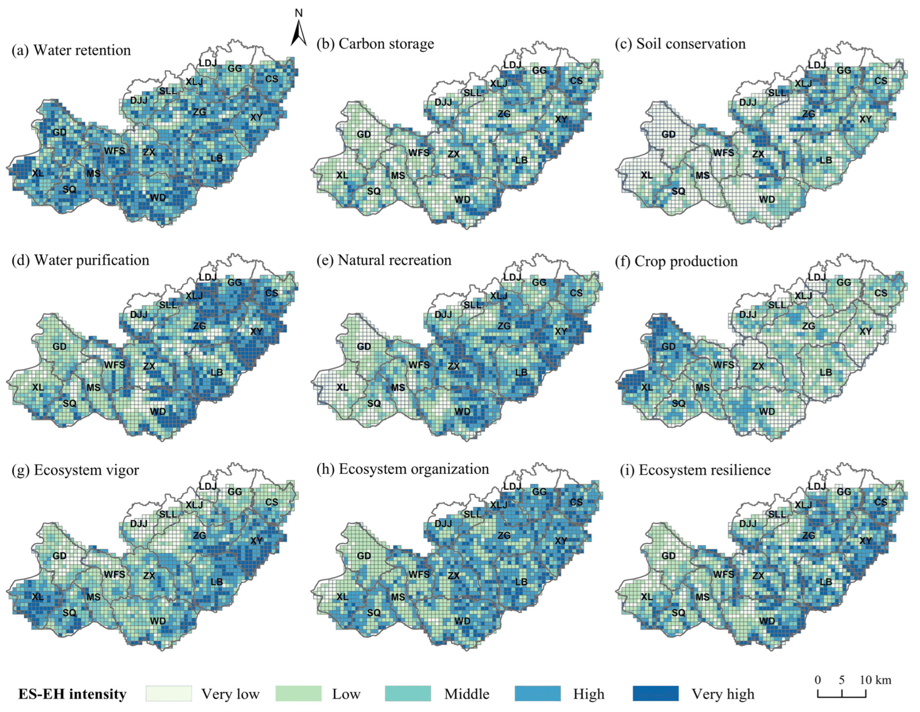
4.1. Spatial Patterns of ESs and EH Properties

Heterogeneous spatial patterns of different ESs and EH properties were found in the study area (Figure 3). Most grids had middle or above-middle levels of water retention, while a small cluster with a very low level of water retention was observed in the northern part of Zhangxia town. Three regulating ESs (carbon storage, soil conservation, and water purification), natural aesthetics and recreation, and ecosystem organization and resilience shared some similarities in terms of the spatial pattern, which exhibited significantly lower values in the western part than those in the eastern part. Moreover, it was found that in the Guide and Xiaoli towns on the western edge of the JMSA, the very low and low levels of these ESs and EH properties covered most of the lands. However, the high and very high levels of these ESs and EH properties were largely located in the mountainous areas, where human activities are restricted and plenty of natural ecosystems are located. By contrast, crop production showed a distinct distribution, where all the grids with a very high level and nearly half of the grids with a high level were located in the western part. This pattern may be explained by the fact that the western region of the JSMA is characterized by flat terrain and fertile soil, which are suitable for agricultural development. In terms of ecosystem vigor, the grids with the very high level were aggregated in the Xiaoli, Shuangquan, Wande, Liubu, Zhonggong, and Xiying towns, while the grids with the very low level of ecosystem vigor were mainly situated in the northern part.

4.2. ES-EH Coupling Coordination Degree

Figure 4a,b illustrate that CESR and EH had uneven spatial distributions in the study area. Based on the quantification of CESR and EH, we calculated the ES-EH coupling coordination degree on the gird scale. The grids with the high ES-EH coupling coordination degree were largely located along the mountains and aggregated in the eastern part. However, the grids with the low coupling coordination degree were mainly located in the areas with flat terrain. We found that the grids with the lowest coupling coordination degree were observed in the Xiaoli, Guide, Wande, Zhangxia, and Zhonggong towns. On the town scale, the towns with the top three average coupling coordination degrees were Xiying, Xinglongjie, and Caishi towns, and the town with the lowest average coupling coordination degree was the Guide town.

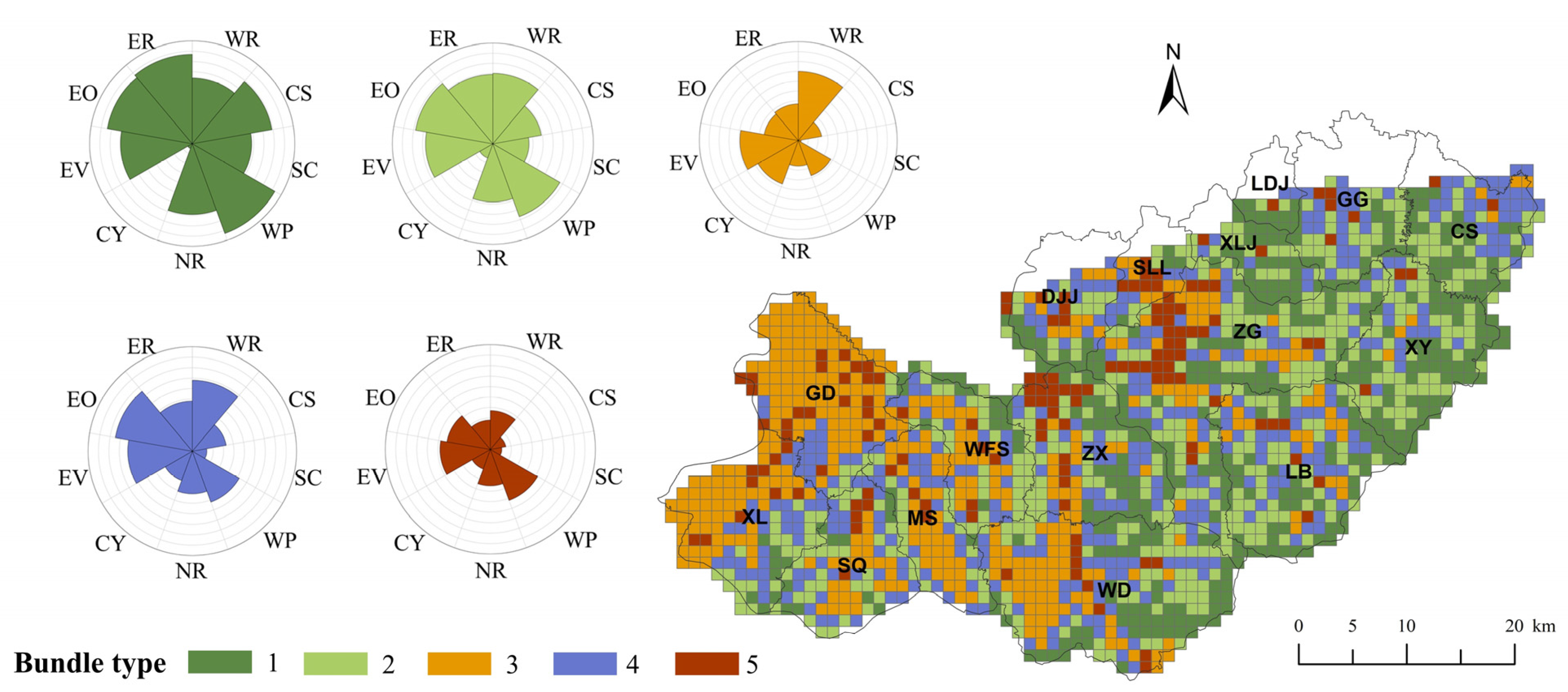
4.3. ES-EH Bundle Identification

Based on clustering analysis, we identified five ES-EH bundle types, which were characterized by distinct ES-EH compositions (Figure 5). We named each bundle type according to its ES-EH composition characteristics.

• Bundle type 1: multifunctionality

This bundle type provided the highest levels of almost all the ESs and EH properties. However, this bundle type had the lowest crop production, which can be explained by the lowest farmland area proportion among the five bundle types. Meanwhile, high evapotranspiration induced by forests in this bundle type had reduced local water retention capacity, which led to a slightly lower water retention capacity than the highest water retention of the five bundle types. Since this bundle type had the most types of ESs and EH properties with the highest values, we named this bundle type “multifunctionality”.

• Bundle type 2: subordinate multifunctionality

This bundle type was featured with high regulating and cultural ESs and EH properties, which was similar to the ES-EH composition of bundle type 1 to some degrees. This bundle had the highest water retention, and the second highest carbon storage, soil conservation, water purification, natural aesthetics and recreation, and EH properties. Considering the similarities and differences between bundle types 1 and 2, we named bundle type 2 “subordinate multifunctionality”.

• Bundle type 3: the highest crop production

Bundle type 3 was mainly located in the western plain areas, and had the highest crop production among the five bundle types. Farmland was the dominant land use type in the regions with bundle type 3, accounting for 80.67% of the total area. However, soil conservation in this bundle was the lowest due to the lack of green spaces and soil erosion management. Furthermore, there were the lowest ecosystem organization and water purification in this bundle type, which can be explained by the landscape homogeneity and high nutrient load caused by intensive agriculture, respectively.

• Bundle type 4: ESs and EH properties of the medium level

This bundle type largely appeared in the junctions of the regions with other bundle types. This bundle type was characterized by medium levels of almost all the ESs and EH properties. The region with bundle type 4 had green spaces of around 26% of the total area, which can provide various regulating and cultural ESs and sustain local EH to some degree.

• Bundle type 5: ESs and EH properties of low levels

This bundle type was mainly located in the human-dominated areas which had the highest population density, GDP level, and urban land proportion. All the ESs and EH properties in this bundle were at low levels. Water retention, carbon storage, and ecosystem vigor and resilience within this bundle type ranked the lowest among the five bundle types, while soil conservation, water purification, natural aesthetics and recreation, and ecosystem organization were the second lowest.

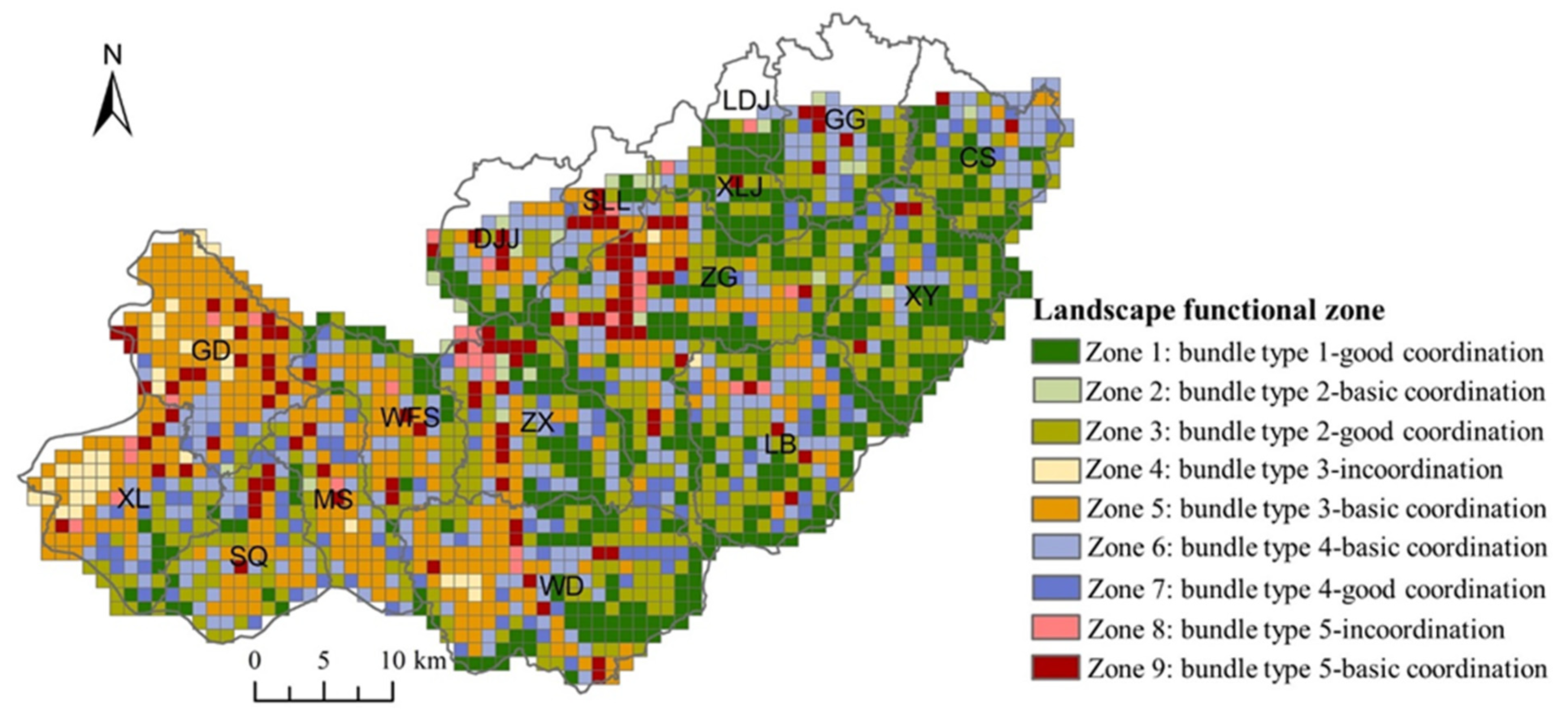
4.4. Landscape Functional Zone Identification

Based on the Jenks classification method, we divided the coupling coordination degrees of all the grids into three classes, i.e., incoordination (low class), basic coordination (medium level), and good coordination (high level). After overlapping the maps of the ES-EH bundle types and coupling coordination classes, we generated nine landscape functional zones (Figure 6).

All the grids with bundle type 1 were in the good coordination class, so the delineated zone 1 was featured with bundle type 1 and good ES-EH coordination. There is no incoordination class for grids with bundle type 2, while most girds with this bundle type belonged to good coordination and the remaining grids belonged to incoordination. Therefore, these grids were divided into two zones, i.e., zones characterized by bundle type 2—basic coordination (zone 2) and bundle type 2—good coordination (zone 3). Grids with bundle type 3 were covered by incoordination and basic coordination classes, and then zone 4 (bundle type 3—incoordination) and zone 5 (bundle type 3—basic coordination) were generated. Grids with bundle type 4 were divided into two zones according to the coupling coordination class, i.e., zone 6 (bundle type 4—basic coordination) and zone 7 (bundle type 5—good coordination). Finally, grids with bundle type 5 fell into the classes of incoordination and basic coordination, and thus were divided into zone 8 (bundle type 5—incoordination) and zone 9 (bundle type 5—basic coordination). In general, zone 3 was the largest one, accounting for 24.68% of the total area. Zones with the second and third largest areas were zones 1 and 5, while zone 2 had the smallest area among the nine zones, which only made up 1.24% of the total area.

5. Discussion

5.1. Advantages of Landscape Functional Zoning Proposed in This Study

5.1.1. Integrating ES and EH Information into the Design Stage of Landscape Planning

Recently, a growing number of researchers have realized the importance of linking ESs to EH in ecosystem management [24]. Without considering the health and integrity of ecosystems, the ES concept can lead to unintended trade-offs between satisfying human demands and the intrinsic values of ecosystems [58]. EH was proposed to link those important ecosystem properties and processes to ecosystem management, and can overcome the potential drawbacks of landscape planning solely relying upon the ES framework [24]. The number of empirical studies linking the ES and EH has increased recently, such as the case studies of urban agglomerations [48] and mountainous regions [59]. However, the main purpose of the previous studies linking EH to ES is ecosystem monitoring, but how to incorporate the EH and ES into the design stage of landscape planning, e.g., spatial zoning, is rarely answered. We delineated landscape management zones according to the spatially explicit information about the ES and EH, which can enable decision-makers to manage ESs and EH together. By our zoning method, the EH properties obtain as much attention as ESs do, which can help planners manage EH properties in ES-based planning. For example, EH properties with high intensities in one specific zone can be highlighted for potential conservation actions (e.g., ecosystem organization in zone 1), while EH properties of very low levels indicate the necessity of restoration (e.g., ecosystem organization in zones 4 and 5). Furthermore, the simultaneous representation of ESs and EH properties (i.e., the ES-EH composition) in the bundle form in each zone can support the decision making of multi-objectives. This zoning can help planners formulate innovative solutions where ESs and EH properties can be improved and maintained together in the early planning stage.

5.1.2. Coupling Coordination as a Novel Approach to Evaluate the Overall Status of ES and EH Subsystems

Landscape planning is required to promote EH and ES together [60], so the win–win situation between EH and ESs can indicate an ideal state [48]. Some researchers have evaluated the overall ecosystem state of satisfying human demands and maintaining intrinsic values by using the product or summation of multiple ES and EH indicators [61]. However, such calculation methods may not fully reflect the synergy between the ES and EH subsystems. For example, a typical mean of unsustainable ES management is the ES increase at the cost of ecosystem integrity and health [62], but the multiplicative or cumulative calculation may be insensitive to such an unsustainable ecosystem state due to the ignorance of ES-EH interactions. By contrast, coupling coordination analysis can not only indicate the overall performance of ES and EH subsystems, but also represent the interactive relationship between ES and EH subsystems. Recently, coupling coordination analysis has been increasingly used in the ES research field. For example, coupling coordination analysis has been adopted to deepen the understanding of the coordination between ES supply and demand [53], ES and urbanization [63], and ES and other land use functions [64]. The existing studies have shown that the coordination of different subsystems can be considered an important planning goal, and good coordination can thus act as an optimal reference [29]. Therefore, we suggested that the coupling coordination of the ES and EH can indicate the desired ecosystem state, and can be used as an important goal and reference in landscape planning. Furthermore, the ES-EH coupling coordination degree on the grid scale can provide spatially explicit information about ES-EH coupling coordination states, which can support spatially determining the management intensity and priority.

5.1.3. Zoning Based on the ES-EH Composition and Coordination

ES-EH bundle analysis is a promising instrument for landscape management zoning, which minimizes the difference in the ES composition within one bundle and maximizes the difference between different bundles [65]. Therefore, similar planning and management strategies are suggested to be formulated and implemented for units sharing one bundle type [66]. However, few studies have worked on further identifying the ES-EH coupling coordination difference within a single bundle type. In this study, in order to determine landscape functional zones, we not only analyzed the ES-EH bundle, but also performed ES-EH coupling coordination analysis. We found that grids characterized by the same ES-EH composition can be different in coupling coordination classes. The difference in the coupling coordination class for grids indicates that differentiated planning strategies and management intensity within the same bundle type should be considered in landscape planning. For example, in terms of bundle type 2, most of the grids had good ES-EH coordination, while the other grids were in the basic coordination class. Those grids with basic coordination deserve more attention in terms of ecosystem restoration to improve the grids’ coupling coordination status. Overall, zoning based on bundle and coupling coordination analyses can provide more explicit information for decision-makers, which can contribute to making elaborate planning strategies.

5.2. Landscape Planning Implications for Each Zone

ES-EH bundle analysis can illustrate the ES-EH composition in different zones, and thus helps decision-makers determine the dominant ESs/EH properties as conservation targets. Furthermore, ES-EH coupling coordination analysis can provide an overall state of ES-EH coordination, which can support determining the conservation intensity. The basic and good coordination corresponded to the general and high conservation intensities, while the zones with incoordination were assigned with the low conservation intensity. With the support of the ES-EH bundle and coupling coordination analysis, we identified the conservation intensity and target of each zone (

Table 2. Conservation intensity and target of different landscape functional zones.

Landscape Functional Zones	Conservation Target	Conservation Intensity
Zone 1	CS, SC, WP, NR, EV, EO, ER	High intensity
Zone 2	WR, WP, NR, EV, EO, ER	General intensity
Zone 3		High intensity
Zone 4	WR, CY, EV	Not conservation area
Zone 5		General intensity
Zone 6	WR, EV, EO	General intensity
Zone 7		High intensity
Zone 8	/	Low intensity
Zone 9		General intensity

Noted: ES-EH bundle type identification. WR—water retention; CS—carbon sequestration; SC—soil conservation; WP—water purification; NR—natural aesthetics and recreation; CY—crop yield; EV—ecosystem vigor; EO—ecosystem organization; ER—ecosystem resilience.

). Finally, specific landscape planning strategies were made with the consideration of the socio-ecological conditions in different zones. It should be noticed that the zones sharing a similar bundle type had common landscape planning strategies related to the conservation target, while some differentiated strategies were proposed according to the conservation intensity.

In terms of zone 1, this zone was characterized by the multifunctionality bundle type, which represented a set of conservation targets including carbon sequestration, soil retention, water purification, natural aesthetics and recreation, ecosystem vigor, ecosystem organization, and ecosystem resilience. Additionally, this zone had a high conservation intensity. Therefore, we set zone 1 as the core conservation area, which deserves the strictest conservation management and highest conservation investment. We suggested conducting Ecological Red Line, a legal conservation planning scheme in China, in this zone. Urban expansion and intensive human activities are not allowed, and natural ecosystems (including forestland, grassland, and water) should be spatially delineated with official boundary tablets. Managers should afforest with native plant species (such as Platycladus orientalis) and maintain the landscape structure to conserve EH. Considering high natural aesthetics and recreation, ecotourism development with slight human pressure was encouraged. Additionally, zone 1 had the highest soil conservation among the nine zones. To protect soil conservation in this zone, we suggested increasing the vegetation coverage in the areas with steep slopes, and afforestation projects should be promoted (e.g., the Grain for Green Project). Furthermore, the strict conservation regulation can impair the economic welfare of residents, and thus ES payment was suggested to be implemented in zone 1.

In terms of zones 2 and 3, these two zones exhibited the ES-EH composition illustrated by the subordinate multifunctionality bundle type, which indicated the conservation targets of water retention, water purification, natural aesthetics and recreation, ecosystem vigor, ecosystem organization, and ecosystem resilience. These two zones had the highest water retention among the nine zones, and specific management strategies for conserving water retention should be made. First, the grassland in these zones played an important role in water retention, because grassland has high water storage capacity but low evapotranspiration. The grassland should be protected from human activities. The grazing intensity should be strictly controlled, and the rest of the grazing system should be constructed to avoid grassland degradation. Second, considering the high value of water retention in these zones, agricultural expansion, which can lead to great non-point source pollution, should be limited to clear water resources. Furthermore, zone 2 should be set as the core conservation area, and some strategies for zone 1, e.g., the control of urban expansion, human activities, ES payment, and conserving native plant species, are also applicable to zone 2.

Zones 4 and 5 had the high levels of crop production and water retention. These two zones were featured with intensive agricultural development, and played an important role in local food security. First, the strictest farmland protection (e.g., Farmland Red Line in China) should be implemented in these two zones, and the conversion from farmlands to built-up lands should be controlled. Meanwhile, farmland reclamation is necessary to improve crop yield [67]. Second, high water retention should be taken good care of to meet the water resource demand induced by agricultural development. Therefore, drainage system and water conservation facility should be constructed. Furthermore, zone 5 had the ES-EH incoordination class, which indicated the unsustainable ecosystem trajectory and thus necessity of ecological restoration. In zone 5, non-production perennial vegetation in the farmland should be cultivated to improve EH and regulating ESs simultaneously [68]. For instance, hedgerows along the river and road can not only improve landscape connectivity, but also effectively improve soil retention and water purification [69].

Zones 6 and 7 were featured with a high level of ecosystem organization and middle levels of ESs and other EH properties. These zones were mainly located on the fringe of the urban area, and were characterized by heterogeneous landscapes. However, there were great demands for urban and agricultural expansion in these zones, which can lead to landscape homogeneity and consequent ecosystem organization reduction. Therefore, the spatial planning policies related to urban expansion control should be implemented, e.g., the official urban land quota setting and urban growth boundary. Furthermore, we suggested that the agroforestry system should be developed. The agroforestry system can not only meet residents’ demands for agricultural activities, but can also provide multiple regulating ESs and increase EH. Furthermore, zone 7 exhibited good ES-EH coordination, indicating that compared with zone 6, zone 7 should be a conservation priority and receive more conservation investment.

Zone 8 and 9 belonged to bundle type 5, which exhibited the lowest level of most ESs and EH properties. These two zones had the highest population density and GDP, and were located in the urban area. In these two zones, urban green infrastructure needed to be developed. The different types of green infrastructure with the small land occupation were suggested to be planned, e.g., the pocket park, roof garden, and vertical planting. Furthermore, the built-up land with low efficiency in these two zones should be gradually removed or merged, so as to provide more available land for developing green infrastructure. The intensity of human activities should also be controlled to preserve remnant natural ecosystems in the urban area. Additionally, compared with zone 9, zone 9 exhibited worse performance in terms of ecological sustainability indicated by the ES-EH incoordination. Therefore, the intensity of green infrastructure development in zone 8 should be higher.

5.3. Limitations and Future Studies

Although the zoning method proposed in this study has clear implications for landscape planning, there are still several limitations that need to be resolved in future studies. First, there are some uncertainties in determining the weights of ES and EH subsystems in the coupling coordination degree equation. In this study, we assumed that the ES and EH are core parts of ecosystem properties with the same importance, which may vary with regions with different socio-ecological conditions. For example, the ES subsystem may play a more important role than the EH subsystem in a human-dominant landscape, while the EH system can have higher management necessity than the ES subsystem in eco-fragile areas. Further studies on determining the influence coefficient of the ES and EH can be performed considering local stakeholders and conditions. Second, we only validated the water purification value due to data limitations. The local decision-makers have to realize such uncertainty of ES evaluation, and we suggested that future studies should conduct the validation of ES and EH evaluation based on data availability. Another limitation is that our zoning method is mainly for the current ES-EH situation, which did not consider the temporal changes in ESs and EH properties. Further studies can investigate the conversion between different zones in the past or future, which can provide more information for adapted management. Finally, landscapes are not only involved with ecosystems, but are also constituted by socioeconomic systems. Some land use functions relying on socioeconomic systems, e.g., transportation and human living, may have trade-offs with ESs and EH properties provided by ecosystems [13]. We suggested that these land use functions can be further analyzed together with the ES and EH to achieve coordination between ecosystems and socioeconomic systems for regional sustainability.

6. Conclusions

For the synergic management of the ES and EH, this study investigated the method to identify landscape functional zones based on the ES-EH bundle and coupling coordination status. We first quantified ESs and EH properties, and found that three regulating services (soil retention, carbon sequestration, and water purification), natural aesthetics and recreation, and two EH properties (ecosystem organization and resilience) exhibited similar spatial patterns, where the values in the western part were lower than those in the eastern part of the JSMA. However, crop production showed an opposite distribution with high values in the western plain areas. We found that high values of the ES-EH coupling coordination degree were aggregated in the mountainous areas, and Xiying, Xinglongjie, and Caishi towns exhibited the highest coupling coordination degree. Moreover, five ES-EH bundle types were identified based on their ES-EH characteristics, i.e., multifunctionality, subordinate multifunctionality, the highest crop production, ESs and EH properties of the medium level, and ESs and EH properties of low levels. We identified nine landscape management zones according to the characteristics of ES-EH bundle types and the coupling coordination class of all the grids, which can illustrate the ES-EH composition and coordination for each zone. Thereafter, specific landscape management strategies were formulated based on the socio-ecological conditions of each zone. This study provides a novel landscape functional zoning method which integrates the ES and EH in the design stage of landscape planning for the management of ESs and EH properties simultaneously. Future research may further consider the temporal change and include the landscape function depending on socioeconomic systems in our zoning method.

References

1. Pereira, H.M.; Martins, I.S.; Rosa, I.M.; Kim, H.; Leadley, P.; Popp, A.; van Vuuren, D.P.; Hurtt, G.; Quoss, L.; Arneth, A.; et al. Global trends and scenarios for terrestrial biodiversity and ecosystem services from 1900 to 2050. Science 2024, 384, 458–465. [Google Scholar] [CrossRef] [PubMed]
2. Kaletova, T.; Rodriguez-Lozano, P.; Berger, E.; Filipe, A.F.; Logar, I.; Alves, M.H.; Calleja, E.J.; Jorda-Capdevila, D. Considering temporal flow variability of non-perennial rivers in assessing ecosystem service provision. Ecosyst. Serv. 2021, 52, 101368. [Google Scholar] [CrossRef]
3. Mandle, L.; Tallis, H.; Sotomayor, L.; Vogl, A.L. Who loses? Tracking ecosystem service redistribution from road development and mitigation in the Peruvian Amazon. Front. Ecol. Environ. 2015, 13, 309–315. [Google Scholar] [CrossRef]
4. Remme, R.P.; Frumkin, H.; Guerry, A.D.; King, A.C.; Mandle, L.; Sarabu, C.; Bratman, G.N.; Giles-Corti, B.; Hamel, P.; Han, B.; et al. An ecosystem service perspective on urban nature, physical activity, and health. Proc. Natl. Acad. Sci. USA 2021, 118, e2018472118. [Google Scholar] [CrossRef]
5. Folke, C.; Carpenter, S.; Walker, B.; Scheffer, M.; Elmqvist, T.; Gunderson, L.; Holling, C.S. Regime shifts, resilience, and biodiversity in ecosystem management. Annu. Rev. Ecol. Evol. Syst. 2004, 35, 557–581. [Google Scholar] [CrossRef]
6. Costanza, R.; de Groot, R.; Braat, L.; Kubiszewski, I.; Fioramonti, L.; Sutton, P.; Farber, S.; Grasso, M. Twenty years of ecosystem services: How far have we come and how far do we still need to go? Ecosyst. Serv. 2017, 28, 1–16. [Google Scholar] [CrossRef]
7. Vaz, A.S.; Amorim, F.; Pereira, P.; Antunes, S.; Rebelo, H.; Oliveira, N.G. Integrating conservation targets and ecosystem services in landscape spatial planning from Portugal. Landsc. Urban Plan. 2021, 215, 104213. [Google Scholar] [CrossRef]
8. Peng, J.; Xia, P.; Liu, Y.; Xu, Z.; Zheng, H.; Lan, T.; Yu, S. Ecosystem services research: From golden era to next crossing. Trans. Earth Environ. Sustain. 2023, 1, 9–19. [Google Scholar] [CrossRef]
9. Lourdes, K.T.; Hamel, P.; Gibbins, C.N.; Sanusi, R.; Azhar, B.; Lechner, A.M. Planning for green infrastructure using multiple urban ecosystem service models and multicriteria analysis. Landsc. Urban Plan. 2022, 226, 104500. [Google Scholar] [CrossRef]
10. Aziz, T. Terrestrial protected areas: Understanding the spatial variation of potential and realized ecosystem services. J. Environ. Manag. 2023, 326, 116803. [Google Scholar] [CrossRef]
11. Sun, X.; Ma, Q.; Fang, G. Spatial scaling of land use/land cover and ecosystem services across urban hierarchical levels: Patterns and relationships. Landsc. Ecol. 2023, 38, 753–777. [Google Scholar] [CrossRef]
12. Assis, J.C.; Hohlenwerger, C.; Metzger, J.P.; Rhodes, J.R.; Duarte, G.T.; da Silva, R.A.; Boesing, A.L.; Prist, P.R.; Ribeiro, M.C. Linking landscape structure and ecosystem service flow. Ecosyst. Serv. 2023, 62, 101535. [Google Scholar] [CrossRef]
13. Zhang, J.; Li, S.; Lin, N.; Lin, Y.; Yuan, S.; Zhang, L.; Zhu, J.; Wang, K.; Gan, M.; Zhu, C. Spatial identification and trade-off analysis of land use functions improve spatial zoning management in rapid urbanized areas, China. Land Use Policy 2022, 116, 106058. [Google Scholar] [CrossRef]
14. Tran, D.X.; Pearson, D.; Palmer, A.; Lowry, J.; Gray, D.; Dominati, E.J. Quantifying spatial non-stationarity in the relationship between landscape structure and the provision of ecosystem services: An example in the New Zealand hill country. Sci. Total Environ. 2022, 808, 152126. [Google Scholar] [CrossRef] [PubMed]
15. Li, K.; Hou, Y.; Andersen, P.S.; Xin, R.; Rong, Y.; Skov-Petersen, H. An ecological perspective for understanding regional integration based on ecosystem service budgets, bundles, and flows: A case study of the Jinan metropolitan area in China. J. Environ. Manag. 2022, 305, 114371. [Google Scholar] [CrossRef] [PubMed]
16. Xu, Z.; Peng, J.; Dong, J.; Liu, Y.; Liu, Q.; Lyu, D.; Qiao, R.; Zhang, Z. Spatial correlation between the changes of ecosystem service supply and demand: An ecological zoning approach. Landsc. Urban Plan. 2022, 217, 104258. [Google Scholar] [CrossRef]
17. Liu, Y.; Li, T.; Zhao, W.; Wang, S.; Fu, B. Landscape functional zoning at a county level based on ecosystem services bundle: Methods comparison and management indication. J. Environ. Manag. 2019, 249, 109315. [Google Scholar] [CrossRef]
18. Nie, X.; Lu, B.; Chen, Z.; Yang, Y.; Chen, S.; Chen, Z.; Wang, H. Increase or decrease? Integrating the CLUMondo and InVEST models to assess the impact of the implementation of the Major Function Oriented Zone planning on carbon storage. Ecol. Indic. 2020, 118, 106708. [Google Scholar] [CrossRef]
19. Xia, H.; Yuan, S.; Prishchepov, A.V. Spatial-temporal heterogeneity of ecosystem service interactions and their social-ecological drivers: Implications for spatial planning and management. Resour. Conserv. Recycl. 2023, 189, 106767. [Google Scholar] [CrossRef]
20. Yang, Y.; Zheng, H.; Kong, L.; Huang, B.; Xu, W.; Ouyang, Z. Mapping ecosystem services bundles to detect high- and low-value ecosystem services areas for land use management. J. Clean. Prod. 2019, 225, 11–17. [Google Scholar] [CrossRef]
21. Lanzas, M.; Hermoso, V.; de-Miguel, S.; Bota, G.; Brotons, L. Designing a network of green infrastructure to enhance the conservation value of protected areas and maintain ecosystem services. Sci. Total Environ. 2019, 651, 541–550. [Google Scholar] [CrossRef] [PubMed]
22. Das, M.; Das, A.; Pereira, P.; Mandal, A. Exploring the spatio-temporal dynamics of ecosystem health: A study on a rapidly urbanizing metropolitan area of Lower Gangetic Plain, India. Ecol. Indic. 2021, 125, 107584. [Google Scholar] [CrossRef]
23. Qiao, W.; Huang, X. The impact of land urbanization on ecosystem health in the Yangtze River Delta urban agglomerations, China. Cities 2022, 130, 103981. [Google Scholar] [CrossRef]
24. Müller, F.; Burkhard, B.; Kandziora, M.; Schimming, C.; Windhorst, W. Ecological indicators: Ecosystem health. In Biological and Ecological Systems; CRC Press: Boca Raton, FL, USA, 2020; pp. 207–227. [Google Scholar]
25. Das, M.; Das, A.; Mandal, A. Research note: Ecosystem Health (EH) assessment of a rapidly urbanizing metropolitan city region of eastern India–A study on Kolkata Metropolitan Area. Landsc. Urban Plan. 2020, 204, 103938. [Google Scholar] [CrossRef]
26. Paetzold, A.; Warren, P.H.; Maltby, L.L. A framework for assessing ecological quality based on ecosystem services. Ecol. Complex. 2010, 7, 273–281. [Google Scholar] [CrossRef]
27. Zhao, X.; Huang, G. Urban watershed ecosystem health assessment and ecological management zoning based on landscape pattern and SWMM simulation: A case study of Yangmei River Basin. Environ. Impact Assess. Rev. 2022, 95, 106794. [Google Scholar] [CrossRef]
28. Li, K.; Hou, Y.; Andersen, P.S.; Xin, R.; Rong, Y.; Skov-Petersen, H. Identifying the potential areas of afforestation projects using cost-benefit analysis based on ecosystem services and farmland suitability: A case study of the Grain for Green Project in Jinan, China. Sci. Total Environ. 2021, 787, 147542. [Google Scholar] [CrossRef]
29. Zhang, D.; Chen, Y. Evaluation on urban environmental sustainability and coupling coordination among its dimensions: A case study of Shandong Province, China. Sustain. Cities Soc. 2021, 75, 103351. [Google Scholar] [CrossRef]
30. Zhou Xu, J.; Lin, Z. Conflict or coordination? Assessing land use multi-functionalization using production-living-ecology analysis. Sci. Total Environ. 2017, 577, 136–147. [Google Scholar] [CrossRef]
31. Cusens, J.; Barraclough, A.D.; Måren, I.E. Integration matters: Combining socio-cultural and biophysical methods for mapping ecosystem service bundles. Ambio 2023, 52, 1004–1021. [Google Scholar] [CrossRef]
32. Yohannes, H.; Soromessa, T.; Argaw, M.; Warkineh, B. Spatio-temporal changes in ecosystem service bundles and hotspots in Beressa watershed of the Ethiopian highlands: Implications for landscape management. Environ. Chall. 2021, 5, 100324. [Google Scholar] [CrossRef]
33. Dittrich, A.; Seppelt, R.; Václavík, T.; Cord, A.F. Integrating ecosystem service bundles and socio-environmental conditions—A national scale analysis from Germany. Ecosyst. Serv. 2017, 28, 273–282. [Google Scholar] [CrossRef]
34. Jiangting, W.; Jinghui, S.; Yuan, Y.; Zhenjiang, C.; Zhenghe, X.U.; Lirong, X.U. Research on Characteristics of Soil Erosion in the Southern Mountainous Area of Jinan City Based on Scale Transformation. Yellow River 2017, 36, 122–127. [Google Scholar]
35. Yang, H.; Shao, X.; Wu, M. A review on ecosystem health research: A visualization based on CiteSpace. Sustainability 2019, 11, 4908. [Google Scholar] [CrossRef]
36. Haines-Young, R.; Potschin-Young, M. Revision of the Common International Classification for Ecosystem Services (CICES V5.1): A Policy Brief. One Ecosyst. 2018, 3, e27108. [Google Scholar] [CrossRef]
37. Sine, W.; Caitong, L.; Yutong, L. Ecological Restoration of Dam aged Urban Mountains—A Case Study on Plant Restoration of Southern Mountainous Area of Jinan City. Anhui For. Sci. Technol. 2017, 43, 46–49. [Google Scholar]
38. Chang, X.; Xu, Z.; Zhao, G.; Cheng, T.; Song, S. Spatial and temporal variations of precipitation during 1979–2015 in Jinan City, China. J. Water Clim. Chang. 2018, 9, 540–554. [Google Scholar] [CrossRef]
39. Sharp, R.; Tallis, H.; Ricketts, T.; Guerry, A.; Wood, S.; Chaplin-Kramer, R.; Nelson, E.; Ennaanay, D.; Wolny, S.; Olwero, N. InVEST User’s Guide; The Natural Capital Project, Stanford University: Stanford, CA, USA, 2014. [Google Scholar]
40. Tian, S.; Wu, W.; Shen, Z.; Wang, J.; Liu, X.; Li, L.; Li, X.; Liu, X.; Chen, H. A cross-scale study on the relationship between urban expansion and ecosystem services in China. J. Environ. Manag. 2022, 319, 115774. [Google Scholar] [CrossRef]
41. Rong, Y.; Li, K.; Guo, J.; Zheng, L.; Luo, Y.; Yan, Y.; Wang, C.; Zhao, C.; Shang, X.; Wang, Z. Multi-scale spatio-temporal analysis of soil conservation service based on MGWR model: A case of Beijing-Tianjin-Hebei, China. Ecol. Indic. 2022, 139, 108946. [Google Scholar] [CrossRef]
42. Trabucchi, M.; Comín, F.A.; O’Farrell, P.J. Hierarchical priority setting for restoration in a watershed in NE Spain, based on assessments of soil erosion and ecosystem services. Reg. Environ. Chang. 2013, 13, 911–926. [Google Scholar] [CrossRef]
43. Wu, Y.; Tao, Y.; Yang, G.; Ou, W.; Pueppke, S.; Sun, X.; Chen, G.; Tao, Q. Impact of land use change on multiple ecosystem services in the rapidly urbanizing Kunshan City of China: Past trajectories and future projections. Land Use Policy 2019, 85, 419–427. [Google Scholar] [CrossRef]
44. Dou, H.; Li, X.; Li, S.; Dang, D. How to Detect Scale Effect of Ecosystem Services Supply? A Comprehensive Insight from Xilinhot in Inner Mongolia, China. Sustainability 2018, 10, 3654. [Google Scholar] [CrossRef]
45. Cui, F.; Tang, H.; Zhang, Q.; Wang, B.; Dai, L. Integrating ecosystem services supply and demand into optimized management at different scales: A case study in Hulunbuir, China. Ecosyst. Serv. 2019, 39, 100984. [Google Scholar] [CrossRef]
46. Cao, Y.; Cao, Y.; Li, G.; Tian, Y.; Fang, X.; Li, Y.; Tan, Y. Linking ecosystem services trade-offs, bundles and hotspot identification with cropland management in the coastal Hangzhou Bay area of China. Land Use Policy 2020, 97, 104689. [Google Scholar] [CrossRef]
47. Xie, X.; Fang, B.; Xu, H.; He, S.; Li, X. Study on the coordinated relationship between Urban Land use efficiency and ecosystem health in China. Land Use Policy 2021, 102, 105235. [Google Scholar] [CrossRef]
48. Pan, Z.; He, J.; Liu, D.; Wang, J.; Guo, X. Ecosystem health assessment based on ecological integrity and ecosystem services demand in the Middle Reaches of the Yangtze River Economic Belt, China. Sci. Total Environ. 2021, 774, 144837. [Google Scholar] [CrossRef]
49. Xiao, R.; Liu, Y.; Fei, X.; Yu, W.; Zhang, Z.; Meng, Q. Ecosystem health assessment: A comprehensive and detailed analysis of the case study in coastal metropolitan region, eastern China. Ecol. Indic. 2019, 98, 363–376. [Google Scholar] [CrossRef]
50. Wilson, J.S.; Clay, M.; Martin, E.; Stuckey, D.; Vedder-Risch, K. Evaluating environmental influences of zoning in urban ecosystems with remote sensing. Remote Sens. Environ. 2003, 86, 303–321. [Google Scholar] [CrossRef]
51. Li, K.; Hou, Y.; Fu, Q.; Randall, M.T.; Andersen, P.S.; Qiu, M.; Skov-Petersen, H. Integrating decision-making preferences into ecosystem service conservation area identification: A case study of water-related ecosystem services in the Dawen River watershed, China. J. Environ. Manag. 2023, 340, 117972. [Google Scholar] [CrossRef]
52. Rapport, D.J.; Costanza, R.; McMichael, A.J. Assessing ecosystem health. Trends Ecol. Evol. 1998, 13, 397–402. [Google Scholar] [CrossRef]
53. Sun, X.; Jiang, Z.; Liu, F.; Zhang, D. Monitoring spatio-temporal dynamics of habitat quality in Nansihu Lake basin, eastern China, from 1980 to 2015. Ecol. Indic. 2019, 102, 716–723. [Google Scholar] [CrossRef]
54. Yang, M.; Zhao, X.; Wu, P.; Hu, P.; Gao, X. Quantification and spatially explicit driving forces of the incoordination between ecosystem service supply and social demand at a regional scale. Ecol. Indic. 2022, 137, 108764. [Google Scholar] [CrossRef]
55. Gou, M.; Li, L.; Ouyang, S.; Wang, N.; La, L.; Liu, C.; Xiao, W. Identifying and analyzing ecosystem service bundles and their socioecological drivers in the Three Gorges Reservoir Area. J. Clean. Prod. 2021, 307, 127208. [Google Scholar] [CrossRef]
56. Zhao, M.; Peng, J.; Liu, Y.; Li, T.; Wang, Y. Mapping Watershed-Level Ecosystem Service Bundles in the Pearl River Delta, China. Ecol. Econ. 2018, 152, 106–117. [Google Scholar] [CrossRef]
57. Gong, J.; Cao, E.; Xie, Y.; Xu, C.; Li, H.; Yan, L. Integrating ecosystem services and landscape ecological risk into adaptive management: Insights from a western mountain-basin area, China. J. Environ. Manag. 2021, 281, 111817. [Google Scholar] [CrossRef]
58. Burkhard, B.; Kroll, F.; Nedkov, S.; Müller, F. Mapping ecosystem service supply, demand and budgets. Ecol. Indic. 2012, 21, 17–29. [Google Scholar] [CrossRef]
59. Xiao, Y.; Guo, L.; Sang, W. Impact of fast urbanization on ecosystem health in mountainous regions of southwest China. Int. J. Environ. Res. Public Health 2020, 17, 826. [Google Scholar] [CrossRef]
60. Tzoulas, K.; Korpela, K.; Venn, S.; Yli-Pelkonen, V.; Kaźmierczak, A.; Niemela, J.; James, P. Promoting ecosystem and human health in urban areas using Green Infrastructure: A literature review. Landsc. Urban Plan. 2007, 81, 167–178. [Google Scholar] [CrossRef]
61. Kang, P.; Chen, W.; Hou, Y.; Li, Y. Linking ecosystem services and ecosystem health to ecological risk assessment: A case study of the Beijing-Tianjin-Hebei urban agglomeration. Sci. Total Environ. 2018, 636, 1442–1454. [Google Scholar] [CrossRef]
62. Villamagna, A.M.; Angermeier, P.L.; Bennett, E.M. Capacity, pressure, demand, and flow: A conceptual framework for analyzing ecosystem service provision and delivery. Ecol. Complex. 2013, 15, 114–121. [Google Scholar] [CrossRef]
63. Liu, N.; Liu, C.; Xia, Y.; Da, B. Examining the coordination between urbanization and eco-environment using coupling and spatial analyses: A case study in China. Ecol. Indic. 2018, 93, 1163–1175. [Google Scholar] [CrossRef]
64. Li, J.; Sun, W.; Li, M.; Meng, L. Coupling coordination degree of production, living and ecological spaces and its influencing factors in the Yellow River Basin. J. Clean. Prod. 2021, 298, 126803. [Google Scholar] [CrossRef]
65. Queiroz, C.; Meacham, M.; Richter, K.; Norström, A.V.; Andersson, E.; Norberg, J.; Peterson, G. Mapping bundles of ecosystem services reveals distinct types of multifunctionality within a Swedish landscape. Ambio 2015, 44, 89–101. [Google Scholar] [CrossRef]
66. Orsi, F.; Ciolli, M.; Primmer, E.; Varumo, L.; Geneletti, D. Mapping hotspots and bundles of forest ecosystem services across the European Union. Land Use Policy 2020, 99, 104840. [Google Scholar] [CrossRef]
67. Loos, J.; Batáry, P.; Grass, I.; Westphal, C.; Bänsch, S.; Baillod, A.B.; Hass, A.L.; Rosa, J.; Tscharntke, T. Vulnerability of Ecosystem Services in Farmland Depends on Landscape Management. In Atlas of Ecosystem Services; Springer: Berlin/Heidelberg, Germany, 2019; pp. 91–96. [Google Scholar]
68. Rallings, A.M.; Smukler, S.M.; Gergel, S.E.; Mullinix, K. Towards multifunctional land use in an agricultural landscape: A trade-off and synergy analysis in the Lower Fraser Valley, Canada. Landsc. Urban Plan. 2019, 184, 88–100. [Google Scholar] [CrossRef]
69. Jensen, A.K.; Uggeldahl, K.C.; Jacobsen, B.H.; Jensen, J.D.; Hasler, B. Including aesthetic and recreational values in cost-effectiveness analyses of land use change based nitrogen abatement measures in Denmark. J. Environ. Manag. 2019, 240, 384–393. [Google Scholar] [CrossRef]
Figure 1. The location, elevation, and land use/cover types of the study area.
Land 13 01561 g001
Figure 2. Research design diagram.
Land 13 01561 g002
Figure 3. Spatial patterns of ESs and EH properties. The abbreviation of the town name includes the following: ZG—Zhonggong town; CS—Caishi town; LB—Liubu town; XY—Xiying town; GG—Ganggou town; WD—Wande town; ZX—Zhangxia town; GD—Guide town; WFS—Wufengshan town; LDJ—Longdongjie town; SLL—Shiliuli town; DJJ—Dangjiajie town; XLJ—Xinglongjie town; SQ—Shuangquan town; XL—Xiaoli town; MS—Mashan town.
Land 13 01561 g003
Figure 4. Spatial patterns of CESR, EH, and ES-EH coupling coordination. The abbreviation of the town name includes the following: ZG—Zhonggong town; CS—Caishi town; LB—Liubu town; XY—Xiying town; GG—Ganggou town; WD—Wande town; ZX—Zhangxia town; GD—Guide town; WFS—Wufengshan town; LDJ—Longdongjie town; SLL—Shiliuli town; DJJ—Dangjiajie town; XLJ—Xinglongjie town; SQ—Shuangquan town; XL—Xiaoli town; MS—Mashan town.
Land 13 01561 g004
Figure 5. ES-EH bundle type identification. WR—water retention; CS—carbon sequestration; SC—soil conservation; WP—water purification; NR—natural aesthetics and recreation; CY—crop yield; EV—ecosystem vigor; EO—ecosystem organization; ER—ecosystem resilience. The abbreviation of the town name includes the following: ZG—Zhonggong town; CS—Caishi town; LB—Liubu town; XY—Xiying town; GG—Ganggou town; WD—Wande town; ZX—Zhangxia town; GD—Guide town; WFS—Wufengshan town; LDJ—Longdongjie town; SLL—Shiliuli town; DJJ—Dangjiajie town; XLJ—Xinglongjie town; SQ—Shuangquan town; XL—Xiaoli town; MS—Mashan town.
Land 13 01561 g005
Figure 6. Landscape functional zones. The abbreviation of the town name includes the following: ZG—Zhonggong town; CS—Caishi town; LB—Liubu town; XY—Xiying town; GG—Ganggou town; WD—Wande town; ZX—Zhangxia town; GD—Guide town; WFS—Wufengshan town; LDJ—Longdongjie town; SLL—Shiliuli town; DJJ—Dangjiajie town; XLJ—Xinglongjie town; SQ—Shuangquan town; XL—Xiaoli town; MS—Mashan town.
Land 13 01561 g006