2.3.1. The Research Framework
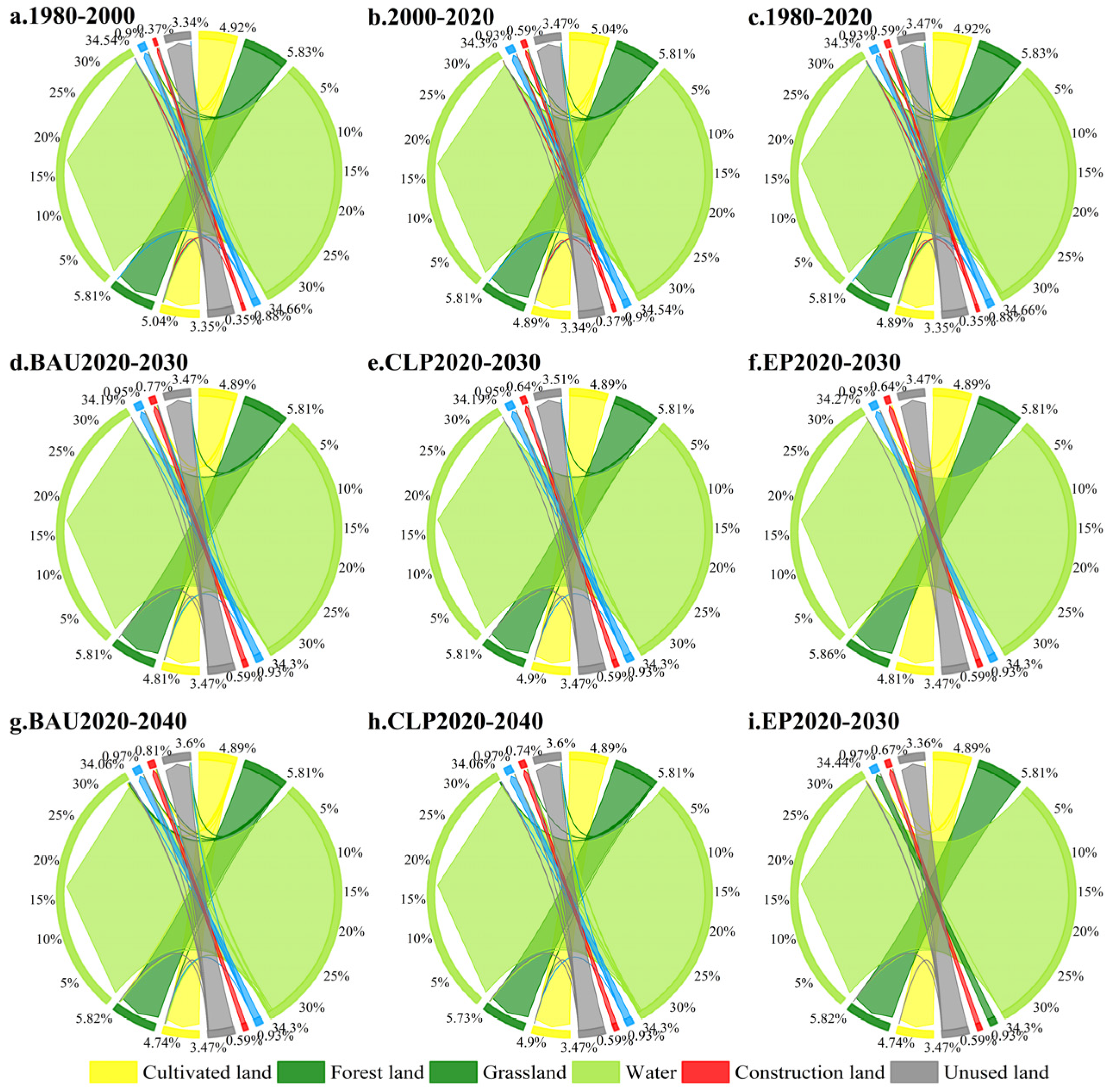
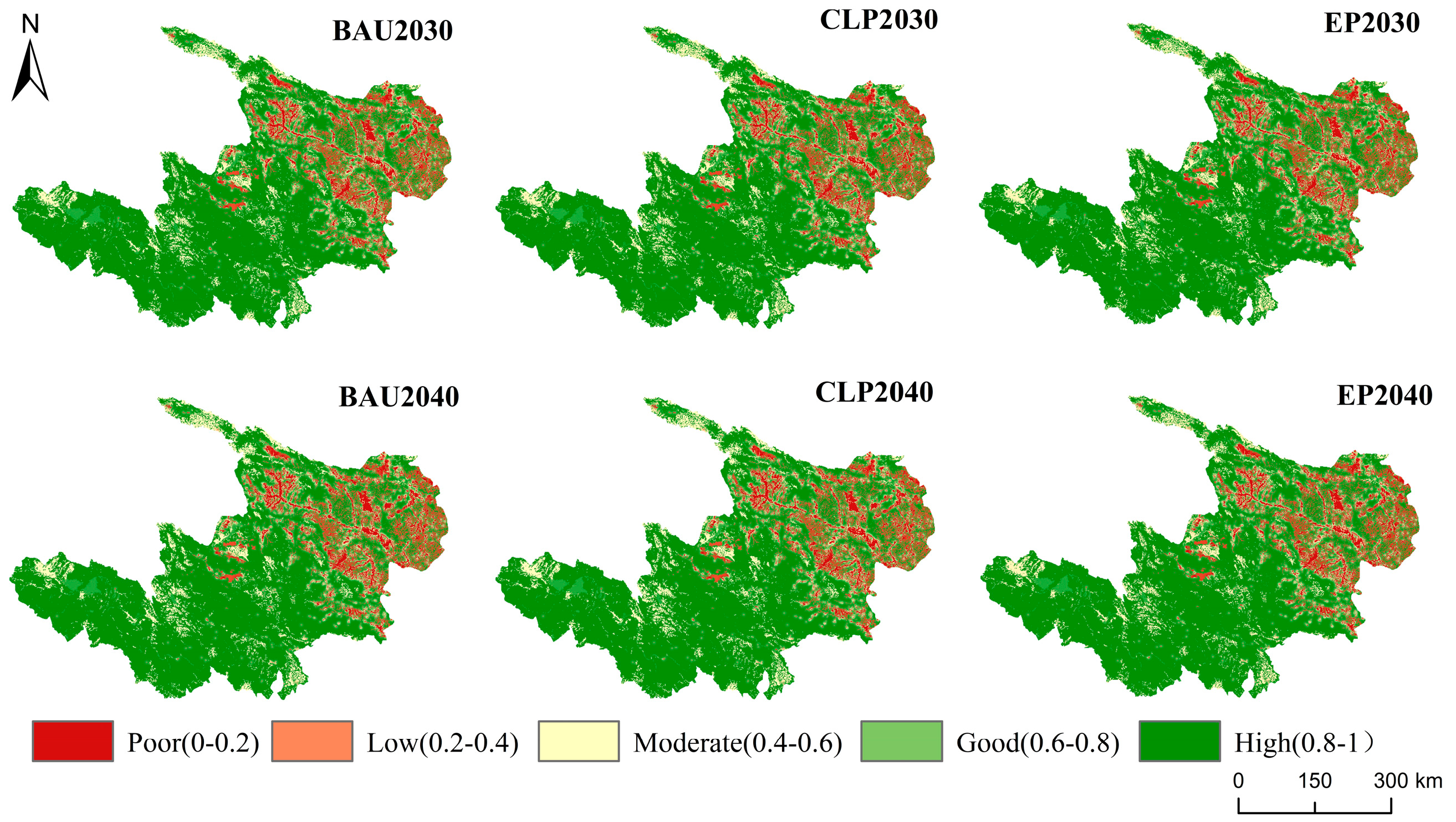
Based on land use data, we obtained the quantity of land use types under different scenarios in 2030 and 2040 using the Markov model. With all the data prepared, we simulated land use patterns in 2030 and 2040 under three scenarios using the FLUS model. Then, we estimated the habitat quality of the Gansu–Qinghai contiguous region of the upper Yellow River during 1980–2040 based on the InVEST model. The research framework is shown in
Figure 2.
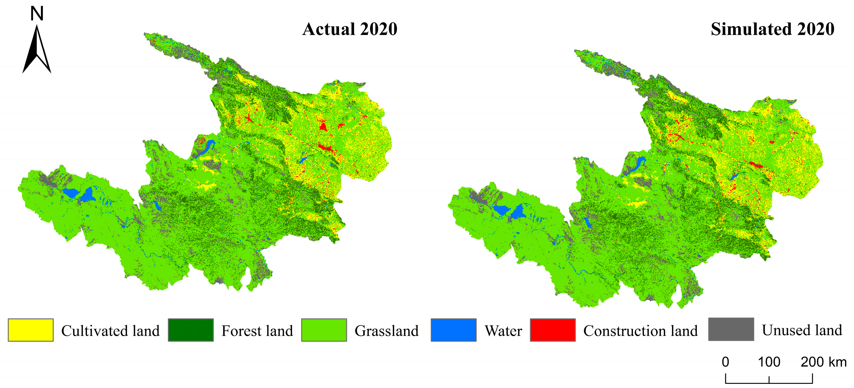
The importance of integrating the FLUS model with the InVEST model lies in their ability to provide complementary information for a more comprehensive understanding of the effects of land use change on ecosystems and their habitat quality. Via this research process, the integration of the FLUS-InVEST model is reflected in the following aspects: First, model construction and calibration. The FLUS model was selected as the land use prediction model and the InVEST model was used to assess habitat quality, and the two models were calibrated and validated using historical data to ensure the accuracy and reliability of the models, which were validated in this study by comparing actual and simulated land use in 2020. Second, the model interface. The outputs of the land use projection model were used as inputs to the habitat quality model, and the projected 2030 and 2040 land use data were used as input data for habitat quality in this study. Third, scenario analysis. Different land use change scenarios were generated using the land use prediction model, and these scenarios were used as inputs to assess the changes in habitat quality under different scenarios through the InVEST model, and the changes in habitat quality under three scenarios were assessed in this study. The effects of different scenarios on habitat quality were analyzed and critical areas were identified.
2.3.2. Scenario Setting
The Gansu–Qinghai contiguous region of the upper Yellow River has diverse climates, different social conditions, and diverse land use patterns. Here is a structured summary of the three scenarios used in the study to predict land use demand and spatial layout in 2040, taking into account different development goals, potential disturbances and policy drivers:
(1) Business as Usual (BAU) Scenario. This scenario assumes the continuation of historical trends in urban expansion without considering national land use planning constraints and policy influences. It is independent of the rate of socio-economic development. It projects that the land use trends from 2020 to 2040 will follow the same patterns observed from 2010 to 2020;
(2) Cultivated Land Priority (CLP) Scenario. The CLP scenario focuses on the protection of basic farmland, imposes strict limitations on the conversion of cultivated land to other land types, and aims to protect cultivated land from being overtaken by urban expansion during economic development. It specifically curtails the transformation of cultivated land to other classes, and sets restrictions on conversions such as forest land to water, grassland to cultivated land, and water to forest land and construction land;
(3) Ecological Priority (EP) Scenario. Under the EP scenario, ecological benefits are prioritized to enhance ecosystem protection and restoration efforts, thereby minimizing the encroachment on ecological lands. With the goal of “restoring important ecosystems and strengthening water conservation functions”, the ecological redline areas are designated as areas where land conversion is prohibited. However, outside the ecological redline areas, the probability of converting arable land, grassland, forest land, and water to construction land is reduced by 35%, 50%, 50%, and 10%, respectively. Ecological land such as forest land, grassland, and water are prohibited from being converted to unused land. At the same time, forest land and water are no longer allowed to be converted to other land use types, while grassland can be converted to forest land and water, but not to other land use types.
2.3.3. FLUS Model
The FLUS model (GeoSOS-FLUS V2.4) is an integrative tool that assimilates both human and natural factors to simulate different land use scenarios [
28,
29]. Initially, the model employs an artificial neural network algorithm to process the baseline period’s land use data and array of driving factors, thereby calculating the suitability probability for each land type. Subsequently, this suitability probability is combined with the neighborhood factor, an adaptive inertia coefficient, and a cost matrix to refine the model’s parameters. Finally, by examining the intricate dynamics of land use alterations under the influence of various driving factors, we can extract simulated outcomes of land use changes [
30].
(1) Estimation of the suitability probability using artificial neural networks
An artificial neural network (ANN) is a machine learning model inspired by biological neural networks [
31]. It has been widely applied in the analysis and simulation of complex, nonlinear problems in geography. An ANN typically involves two key phases: training and prediction. During the training phase, the goal is to determine the appropriate weights for different land use types. In the prediction phase, the objective is to estimate the probability distribution of the spatial arrangement of various land types. The specific formula of an artificial neural network (ANN) is as follows:
where
represents the suitability probability of land use type
on grid
at time
, and
are the adaptive weights between the hidden layer and the output layer, which are fine-tuned during the training process. The term
denotes that neuron
receives signals from all of the input neurons on grid
at time
in the hidden layer. In the output of the neural network, the sum of the suitability probability for all land use types equals 1 for each grid
at each iteration time
.
(2) Cellular automata with an adaptive inertial mechanism
The transition of a land grid to a specific land use type is influenced not only by the occurrence probability but also by various other factors that represent different development states during the forecast period [
32]. The essence of the adaptive inertial competition mechanism lies in the adaptive coefficient. This coefficient modulates the transition probabilities of the current land type in the subsequent iteration to achieve the anticipated developmental objectives.
where
is the coefficient of inertia of land type
. At iteration
and
,
and
are the differences between the requested land quantity for a specific type of land (
) and the actual amount of that land available.
(3) Neighbor factor
The establishment and protection of nature reserves restrict the expansion potential of construction land while bolstering the expansion capabilities of woodlands and grasslands [
33]. To determine the parameters, a comparative analysis of neighborhood factor parameters is conducted before and after the implementation of the current scheme. These neighborhood coefficients quantify the interactions among various land use types. The values of proximity parameter coefficients, which range from 0 to 1, indicate the expansion propensity of land types under the influence of different factors [
34]. A value closer to 1 suggests a stronger ability of a land type to expand. Informed by prior research and the regulatory framework provided by regulations of the People’s Republic of China on Nature Reserves, the Protection Plan of National Key Ecological Function areas and the Land Administration Law of the People’s Republic of China, the neighborhood factor parameters of land use types are set (
Table 2).
(4) Cost transfer matrix for different scenario
The conversion cost matrix quantifies the difficulty associated with the transformation between different land use types [
35]. A value 0 indicates no conversion resistance, and 1 signifies complete convertibility [
36]. Reflecting the dynamics of actual land use changes, the construction cost matrix for construction land is set to 0. This is because, during economic development, other land types are frequently converted into construction land. The cost matrix of other land types is determined based on the conversion constraints that exist among different land types under various scenarios (
Table 3).
(5) Comprehensive probability calculation
The total conversion probability of units occupied by the specified land use type is estimated using the aforementioned factors, including suitability probability, neighborhood factors, suitability matrix, and inertia coefficient, and the formula is as follows [
37]:
where
is the combined probability of conversion from initial land use type to target land use type
at time
;
is the suitability probability of converting pixel
to land use type
k at time
;
is the neighborhood factor of grid
at time
, which affects the conversion of grid
to land use type
;
is the coefficient of inertia of land use type
at time
;
refers to the conversion cost from the initial land use type
to the target land use type
. The land use data for different scenarios are obtained by calculating the probability of each iteration, and the accuracy is verified to finalize the results.
(6) Modeling verification
To ensure the accuracy of the simulation results, the FLUS model was thoroughly validated. The land use data from 2010 served as the baseline for simulating the spatial land use patterns in 2020. To assess the model’s accuracy, 1% of the grid units were randomly selected for evaluation. The simulation achieved an overall accuracy of 98.23%, with a kappa coefficient of 0.9562 and a Figure of Merit (FoM) coefficient of 0.0731. These metrics indicate that the simulated data successfully passed the model verification test, aligning well with the actual land use configurations and the underlying socioeconomic dynamics observed in 2020. Subsequently, multi-scenario spatial simulations were executed.
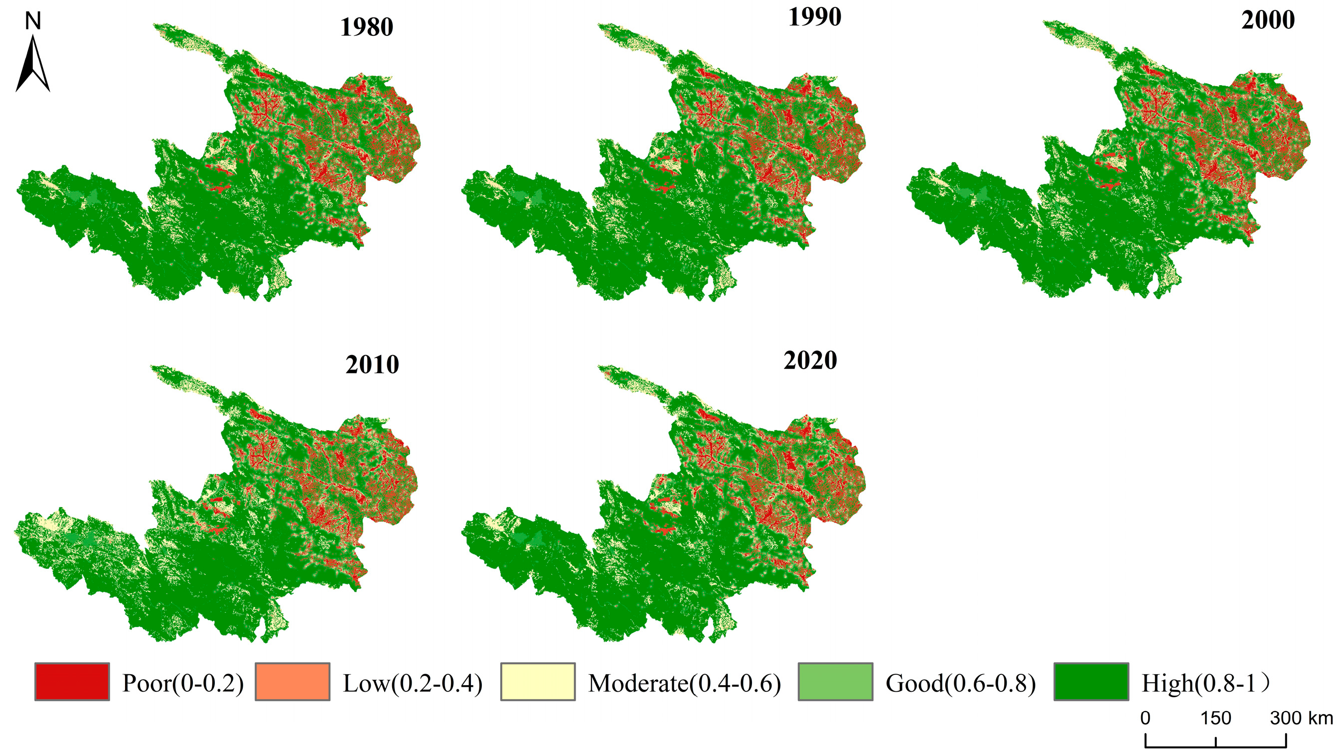
2.3.4. Habitat Quality Assessment
The habitat quality module of the InVSET model (3.14.0) serves as an effective tool for evaluating habitat quality. It operates by processing land use maps and identifying potential threats, with the outcomes indicating how habitat quality responds to land use changes [
38,
39]. In this study, the primary function of the Habitat Quality module (version 3.13.0) involved pinpointing habitat threats and assigning weights to these threats and to habitat sensitivities. This was accomplished through hierarchical analysis, employing expert knowledge (
Table 4), guidance from InVSET user manuals, and relevant studies from the upper Yellow River region. Hierarchical analysis tools were employed to establish the weights for threats and habitat sensitivities. The habitat quality index for a given grid cell
x within land use type
j is calculated as follows:
where
indicates the habitat quality of land use type
in a specific location, with values ranging from 0 to 1, while
is the habitat suitability. The variables
and
refer to normalized constant (
z = 2.5) and half-saturation constant (
k = 0.05), respectively.
To account for the impacts of human activities, the InVEST model incorporates three land use types that are significantly influenced by such activities: cultivated land, construction land and unused land. Additionally, two types of infrastructure, railway and highway, were included as threat factors due to their potential influence on habitats. All input data used to simulate habitat quality, including the maximum stress distance, weight, habitat suitability, and sensitivity of land use types to each threat, were quantitatively analyzed using relevant studies (
Table 5).


