Testing an Algorithm with Asymmetric Markov-Switching GARCH Models in US Stock Trading

Abstract

In the present paper, we extend the current literature in algorithmic trading with Markov-switching models with generalized autoregressive conditional heteroskedastic (MS-GARCH) models. We performed this by using asymmetric log-likelihood functions (LLF) and variance models. From 2 January 2004 to 19 March 2021, we simulated 36 institutional investor’s portfolios. These used homogenous (either symmetric or asymmetric) Gaussian, Student’s t-distribution, or generalized error distribution (GED) and (symmetric or asymmetric) GARCH variance models. By including the impact of stock trading fees and taxes, we found that an institutional investor could outperform the S&P 500 stock index (SP500) if they used the suggested trading algorithm with symmetric homogeneous GED LLF and an asymmetric E-GARCH variance model. The trading algorithm had a simple rule, that is, to invest in the SP500 if the forecast probability of being in a calm or normal regime at t + 1 is higher than 50%. With this configuration in the MS-GARCH model, the simulated portfolios achieved a 324.43% accumulated return, of which the algorithm generated 168.48%. Our results contribute to the discussion on using MS-GARCH models in algorithmic trading with a combination of either symmetric or asymmetric pdfs and variance models.

1. Introduction

Given the current computer and financial econometrics advances in the last 15 years, the modeling of the non-rational behavior among investors and the need for quantitative models to determine trading signs have evolved. This development has led to other ones in algorithmic trading.

Although classical financial economics theories and assumptions do not hold entirely in real life, these have been a good starting point to explain some financial phenomena. Despite this, these theories lack a proper explanation of asset price bubbles or financial market crashes. In some approaches, such as the efficient-market hypothesis [1], these episodes should not exist or are part of atypical situations that should fade in the mid- and long-term. Given this, a potential explanation of these phenomena was proposed by Black [2], who suggested the existence of two types of financial market agents, i.e., (1) the informed traders, who act with a broad and complete information set, and (2) the noisy ones, who lack a proper set and decide according to their sentiment. This explanation led to developing asset pricing models, such as the ones of Fama and French [3,4] or Carhart [5], that extend the original CAPM of Sharpe [6] and Lintner [7]. Fama–French and Carhart models use other factors (along with the market one or stock market benchmark), such as firm size, dividend growth, or even momentum. These two models explain some anomalies that the original capital asset pricing model (CAPM) and the efficient market hypothesis could not [8].

We prefer to use the behavioral asset pricing scope even if the CAPM’s validity and extensions are under discussion. We prefer such perspective, given the lack of explanation of the presence of regimes in financial markets with the classical financial economics ones. Several results show that financial markets have different states of nature not measured in a linear factor model context [9,10,11,12,13]. In addition, the change in such regimes or states of nature results from the sentiment among investors. Given this, Markov-switching models are valuable tools to infer these states of nature and to forecast the probability of being in each regime at $t+n$.

With the developments of behavioral finance as an answer to this need, other asset pricing models extend the classical ones by including market factors such as volatility levels or indexes (the VIX or the VSTOXX indexes) [14,15], the sentiment measured from financial markets, economic or policy news [16,17,18,19], the trends in Google searches, or the news sentiment of financial data news vendors, such as Refinitiv or Bloomberg [20,21]. These sentiment factors allow us to control non-market or non-rational issues and anticipate negative returns proper of distress or market crashes episodes.

The Markov-switching (MS) models are an econometric tool useful to anticipate bubble bursts and market crashes [22,23,24]. These models allow the analyst to estimate location (${\widehat{\mu }}_s$) and scale (${\widehat{\sigma }}_s$) parameters of an $s$ number of regimes or states of nature, e.g., a mean ${\widehat{\mu }}_{s=1}$ and standard deviation ${\widehat{\sigma }}_{s=1}$ for low-volatility or “normal” periods regime ($s=1$) and another (${\widehat{\mu }}_{s=2}$ and ${\widehat{\sigma }}_{s=2}$) for a high-volatility ($s=2$) “distress” or “crisis” one.

Furthermore, as additional outputs of these models, the analyst can estimate the probability ${\xi }_{s,t}$ of being in each regime $s$ at $t$, along with a regime transition probability matrix from $t-1$ to $t$ ($\Pi$). This use has several applications, such as the forecast of recession episodes [22,25,26] or the level of volatility spill-over between financial markets in distress periods [27,28,29,30,31,32].

Among the uses of MS models, we are interested in their application in algorithmic stock trading, that is, quantitative or computer models in which the use of MS models leads to a simple trading sign, i.e., to buy the security or portfolio of interest if the probability of being in a low-volatility or “normal” regime ($s=1$) is high or buying a risk-free asset (or good-performing security in high-volatility periods) otherwise.

This trading rule was primarily suggested by Brooks and Persand [33] and later developed for trading sign and crisis period forecast models [34,35]. These authors mainly tested the benefits of MS models for trading UK stocks in low-volatility or “normal” periods and UK gilts in high-volatility or crisis ones.

Additionally, there are tests of MS models in trading decisions in commodities [36,37], European and US stock markets and volatility futures by using generalized autoregressive conditional heteroskedasticity (GARCH) variances in the estimated MS models (MS-GARCH) [38,39].

These previous works and related ones tested the benefit of MS-GARCH models for trading signs with the following assumptions:

• The marginal probability density function (pdf or pdfs in plural) was homogeneous; this means that the necessary regime-specific pdf to filter ${\xi }_{s,t}$ was the same in all the assumed regimes.
• The used pdfs were the Gaussian, Student’s t, or generalized error density (GED) with symmetric shape.
• The variance model in the MS-GARCH model was symmetric and ignored the potential benefits of including the impact of leverage of negative returns. That is, these tests estimate a regime-specific variance with the same dispersion magnitude, either with positive or negative price returns. Other asymmetric GARCH models, such as the TGARCH [40], the GJRGARCH [41] or the EGARCH [42], have not been tested in an MS-GARCH trading algorithm.
• The variance model in the estimated MS-GARCH models was also homogeneous. That is, the authors assumed that the variance models were the same in each regime.

Other authors suggested the benefit of using asymmetric MS-GARCH models in securities and investment [10,43,44,45,46] to estimate risks. One limitation of relaxing the four previous assumptions is the high computing capabilities needed to backtest each trading period—periods in which the computer estimates the MS or MS-GARCH model and determines and executes a trading sign. This process is fast in a single-date estimation, but to backtest 10 or even 20 years of weekly or daily periods becomes hard computational work.

This considerable effort is due to the potential combinations of heterogeneous symmetric and asymmetric pdfs and high GARCH variances. As a first step, we relaxed assumptions 1 and 3 and simulated the benefits of MS-GARCH with either symmetric or asymmetric pdfs and symmetric or asymmetric GARCH variances. These led us to 36 simulated portfolios with weekly periods from 4 January 2004 to 26 March 2021 (a total of 898 weeks in each MS-GARCH model, totaling 32,329 simulated weeks and 2130.97 h—88.7 days—of simulations). We performed our backtests with a two-core, 1.4 GHz processor, 8 GB (3200 GHz processing) RAM computer.

With these tests, we simulated the performance that an investor would have had, had they used a trading algorithm that estimated the previous trading sign, given the forecast MS or MS-GARCH probability (${\xi }_{s,t+1}$) of being in a high-volatility or distress regime at $t+1$. Our theoretical position is that the assumption of symmetric marginal pdfs and symmetric GARCH variances set aside the potential of more precise trading signs, leading to a more unsatisfactory performance against a trading algorithm that used asymmetric pdfs or asymmetric GARCH variances.

The use of these kinds of asymmetric MS-GARCH trading algorithms could lead to important theoretical and practical implications, such as a trading tool that could weigh the influence of noisy traders and informed ones in a stock-trading strategy.

Our primary rationale was the following: the higher the influence of informed traders in a stock market, the higher the probability of being in a low-volatility regime ($s=1$) at $t+1$ and the better to invest in stocks; further, the higher the presence of noisy traders, the higher the likelihood of being in a distress regime ($s=2$) at $t+1$ and the better to invest in TBILLs.

Additionally, this type of trading algorithm could help make more suitable trading decisions for individual and institutional investors by knowing when to increase or hold their US stock positions or rebalance them to TBILLs.

We ran our trading algorithm and tested its benefit in US stocks (the S&P 500 stocks) and TBILLs from weekly trading decisions from 2004 to 2021.

Our simulation included several distress periods, such as the 2007–2008 financial crisis, the 2013 European debt issues, the 2016–2019 US commercial tensions with China and other countries and the current COVID-19 distress periods (from 2020 to the moment of writing this paper).

Given the above presentation of our theoretical and practical motivations, we offer a brief literature review in the next section.

2. Literature Review

MS models have proved useful for several applications, such as the ones mentioned in the previous section. The original proposal of Hamilton [22,23] allows users to estimate time-fixed parameters for each regime, i.e., a time-fixed parameter set $\theta =\left\{{\widehat{\mu }}_s,{\widehat{\sigma }}_s,{\xi }_s,\Pi \right\}$ with a regime-specific scale and location (${\widehat{\mu }}_s,{\widehat{\sigma }}_s$) parameters. This original proposal also led to extensions such as vector autoregressive models with MS effects (MS-VAR) [47,48,49,50,51]. These models were tested in several spill-over effects [28,31,52,53,54,55,56,57,58] among stock, currency, or commodity markets and between these types of markets. The results from these papers show that the use of MS-VAR models is helpful to estimate and forecast potential contagion effects among markets in high-volatility or crisis periods. These previous works motivate us to predict the probability of a regime change at $t+1$, given a “herd” behavior in distress periods. A behavior that could be proxied not with behavioral finance models and market sentiment proxies but with an econometrics model such as the MS-GARCH.

The original MS model infers, as mentioned, time-fixed location and scale parameters, given the smoothed probability ${\xi }_{s,t}$ filtered according to Hamilton’s [22] algorithm or with Markov chain Monte Carlo (MCMC) estimation with the Metropolis–Hasting algorithm [59]. These filtered probabilities are smoothed according to Kim’s [60] method. Departing from this rationale, the regime-specific location and scale parameters are estimated as follows:

$${\widehat{\mu }}_{s=i}={\displaystyle \sum }_t^T{r}_t\cdot {\xi }_{s=i,t}$$

(1)

$${\widehat{\sigma }}_s^2={\displaystyle \sum }_t^T{\left(r_t-{\widehat{\mu }}_{s=i}\right)}^2\cdot {\xi }_{s=i,t}={\displaystyle \sum }_t^T{\epsilon }_t^2\cdot {\xi }_{s=i,t}$$

(2)

That is, the MS model can estimate the regime-specific location parameter and proxy the risk (standard deviation or scale parameter) in each regime. A drawback of the time-fixed parameters in Equations (1) and (2) is the lack of adaptation to short-term changes in financial markets and security price formation. Departing from this drawback, a natural extension for MS models could be the estimation of Equation (2) in a GARCH context (MS-GARCH models), such as the following:

$${\widehat{\sigma }}_{s,t}^2={\sigma }_0^2+{\displaystyle \sum }_{p=1}^P{\beta }_p\cdot {\epsilon }_{t-p}^2+{\displaystyle \sum }_q^Q{\gamma }_q\cdot {\widehat{\sigma }}_{s,t-q}^2$$

(3)

where ${\epsilon }_t$ are the residuals estimated from a time-fixed location parameter (mean), such as in Equation (1); ${\sigma }_0^2$ is a long-term time-fixed variance level to which ${\widehat{\sigma }}_{s,t}^2$ tends to revert; ${\gamma }_q$ estimates the rate of convergence of ${\widehat{\sigma }}_{s,t}^2$ to ${\sigma }_0^2$; and ${\beta }_p$ estimates the impact that previous exogenous shocks (proxied with jumps in ${\epsilon }_{t-p}^2$) have in the actual short-term variance level. As noted from Equation (3), the location parameter can be estimated for each regime $s$ of interest, leading to extend MS models with a GARCH version of these (MS-GARCH) [47,61,62,63].

The potential use of MS-GARCH models has been widely discussed and tested in several works. The natural use in finance is financial risk measurement, value at risk (VaR), or conditional value at risk (CVaR) estimation [10,29,43,44,64,65,66,67,68,69,70]. MS-GARCH models are suitable for these purposes and trading, as mentioned in the previous section. The original proposal by Brooks and Persand [33] assumed two regimes and a time-fixed location and scale parameter; we consider this, along with Gaussian regime-specific pdfs, a situation that we want to extend in this paper by testing a trading algorithm such as theirs in the US stock market with MS-GARCH models, asymmetric regime-specific pdfs and asymmetric GARCH variances. In their paper, Brooks and Persand (without incorporating stock trading fees) showed that their MS trading algorithm worked appropriately and enhanced an investor’s performance against a buy-and-hold UK stock or Gilt strategy.

Other works, such as De la Torre-Torres et al.’s [36,37,39,71], developed similar tests in the US stock markets, energy and agricultural commodities and even in volatility futures markets. Similar to Brooks and Persand, these authors tested an MS-GARCH trading algorithm. They performed this in a symmetric Gaussian, Student’s t and GED pdf context with symmetric GARCH variances. The simulated portfolios outperformed a buy-and-hold strategy in the simulated stock indexes or commodity futures. The authors incorporated the impact of stock and futures trading fees in these backtests, including roll-over costs. In the specific case of De la Torre-Torres, Galeana-Figueroa and Álvarez-García [39], the authors assumed an MS-GARCH three-regime context. They simulated the performance of a portfolio that invested in European stocks in calm periods ($s=1$), 3-month German Treasury Bills (Bundes) or the 1-month VSTOXX volatility index futures in high-volatility ones. By also including stock trading fees and futures’ roll-over costs, the authors found that using their MS-GARCH trading algorithm (in a two-regime context) is beneficial for outperformance purposes in the short-term. If a given investor wants to outperform a buy-and-hold strategy in European stocks, they must combine the simulated short-term trading strategy with a buy-and-hold one. They must do this by investing in a short-term strategy in calm periods ($s=1$). This last result complements the ones obtained by Alexander and Korovilas [72,73], who found only short-term benefits in a portfolio diversified with volatility futures (in a non-MS or MS-GARCH context).

Other works developed and tested warning systems for high-volatility or distress periods forecasting in the U.S., German, Swiss, or Japanese stock markets [34,35,74]. The authors used financial and economic variables such as the short-term and long-term Treasury yield rate, volatility indexes and corporate bond spreads in these works. Their purpose was to perform logit models that could help to forecast the regime-specific smoothed probabilities ${\widehat{\xi }}_{s,t+1}$ by including the influence of external factors different from the time series of interest. In their results, the authors simulated a portfolio that used their sequential three-regime Gaussian MS smoothed probabilities ${\xi }_{s,t}$ to perform an active trading strategy in the markets of interest. With their results, the authors also found overperformance benefits with the use of MS models.

From these previous works, we want to extend the current literature in the following five ways:

• We want to test if the use of asymmetric regime-specific pdfs adds to smoothed probability forecasts (${\xi }_{s,t+1}$).
• Additionally, we want to test if the use of asymmetric GARCH variances also adds information to the estimated smoothed probabilities ${\xi }_{s,t+1}$. For this case, we used the asymmetric Gaussian, Student’s t and GED pdfs by using Fernández and Steel [75] transformation to induce skewness in the next symmetric Gaussian, Student’s t (with $\nu$ degrees of freedom) and GED (with $\nu$ degrees of freedom and a shape parameter $\lambda$) pdfs, respectively,

  $${\xi }_{s,t}=\frac{1}{\surd 2\pi }{e}^{-\frac{1}{2}{\left(\frac{{\epsilon }_t}{{\sigma }_s}\right)}^2}$$

  (4)

  $${\xi }_{s,t}=\frac{\mathsf{\Gamma }\left(\frac{\nu +1}{2}\right)}{\surd \left(\nu -2\right)\pi \mathsf{\Gamma }\left(\frac{\nu }{2}\right)}{\left(1+\frac{{\left(\frac{{\epsilon }_t}{{\sigma }_s}\right)}^2}{\left(\nu -2\right)}\right)}^{-\frac{\nu +1}{2}},\nu =\mathrm{degrees}\mathrm{of}\mathrm{freedom}$$

  (5)

  $${\xi }_{s,t}=\frac{\nu e^{-\frac{1}{2}{\left|\frac{\left(\frac{{\epsilon }_t}{{\sigma }_s}\right)}{\lambda }\right|}^{\nu }}}{\lambda 2^{\left(1+1/\nu \right)}\mathsf{\Gamma }\left(1/\nu \right)}, \lambda ={\left(\frac{\mathsf{\Gamma }\left(1/\nu \right)}{4^{1/\nu }\mathsf{\Gamma }\left(3/\nu \right)}\right)}^{1/2}$$

  (6)
• We aim to simulate if these asymmetric GARCH variances and marginal pdfs probabilities ${\xi }_{s,t+1}$ lead to better performance against a buy-and-hold strategy in a Standard and Poors 500 (SP500) portfolio.
• We aim to simulate if the asymmetric GARCH and pdf simulated portfolios outperform those simulated with symmetric pdfs and GARCH variances.
• We simulated these portfolios in a homogeneous regime-specific context with the assumption of two volatility regimes. i.e., a low-volatility or “normal” regime ($s=1$) and a high-volatility ($s=2$) or “distress” one.
• We tested if it is better to use more computationally efficient symmetric MS-GARCH models than their asymmetric versions. We conducted this type of testing to give guidelines to the finance industry about the pertinence of asymmetric MS-GARCH models for trading algorithms such as the one tested herein. This result could have an impact on the computational needs for portfolio management or even in high-frequency trading.

For our simulations, we used homogeneous Gaussian, Student’s t-distribution and generalized error distribution (GED) pdfs in the symmetric version of Equations (4)–(6) and the ones achieved with Fernández and Steel [75] transformation. For each two- or three-regime scenario of these six pdfs, we estimated the MS-GARCH models with time-fixed variances, as in Equation (2), or symmetric GARCH ones, as in Equation (3). In addition, we simulated the portfolios with two or three regimes as the previous six pdfs with asymmetric GARCH models, such as the EGARCH of Nelson [42], in Equation (7), the TGARCH of Zakoian [40], in Equation (8), and the GJRGARCH of Glosten, Jaganathan and Runkle [41], in Equation (9).

$$\ln \left({\widehat{\sigma }}_{s,t}^2\right)={\alpha }_{0,s}+{\beta }_{1,s}\cdot \left(\left|{\epsilon }_{t-1}\right|-E\left[{\epsilon }_{t-1}\right]\right)+{\beta }_{2,s}\cdot {\epsilon }_{t-1}+{\gamma }_s\ln \left({\widehat{\sigma }}_{s,t}^2\right)$$

(7)

$${\widehat{\sigma }}_{s,t}^2={\sigma }_{0,s}^2+{\displaystyle \sum }_{p=1}^P(\left[\mathbb{I}\left\{{\epsilon }_{t-1}\ge 0\right\}\cdot {\beta }_{p,s}\right]\cdot {\epsilon }_{t-p}^2-\left[\mathbb{I}\left\{{\epsilon }_{t-1}<0\right\}\cdot {\lambda }_{p,s}\right]\cdot {\epsilon }_{t-p}^2)+{\displaystyle \sum }_q^Q{\gamma }_{q,s}\cdot {\widehat{\sigma }}_{s,t-q}^2$$

(8)

$${\widehat{\sigma }}_{s,t}^2={\sigma }_0^2+{\displaystyle \sum }_{p=1}^P\left[{\beta }_{p,s}+{\lambda }_{p,s}\mathbb{I}\left\{{\epsilon }_{t-1}<0\right\}\right]\cdot {\epsilon }_{t-p}^2+{\displaystyle \sum }_q^Q{\gamma }_q\cdot {\widehat{\sigma }}_{s,t-q}^2$$

(9)

For our simulations, we simulated a theoretical investor that allocated their resources in the SP500 in $s=1$ and in the 3-month TBILLS $s=2$. We decided to use this closed trading strategy by the fact that we simulated 36 possible scenarios with the combinations of the homogeneous pdfs in (4)–(6) and the variance models given in Equations (2) and (7)–(9).

As we mentioned above, our purpose is to test the benefits of using asymmetric pdfs and GARCH variances in the MS-GARCH model estimation process. More specifically, we aim to test the benefit of these asymmetric parameters to make more precise smoothed probabilities forecasts of the low ($s=1$) and high ($s=2$) regime’s smoothed probabilities in a Markov-switching trading algorithm.

The potential practical benefit of our tests is to determine if it is better to use symmetric, computationally more efficient pdfs and GARCH models or more precise but more complex pdfs and GARCH variances. For the case of a private or institutional investor who wants to develop an algorithmic trading system, to know if they can save time in the computer estimation of these models could be of use for latency or accuracy in the investment decision process.

In theoretical terms, we believe that our results will contribute to showing asymmetries in the behavior of financial time series—more specifically, in US stock index risk and algorithmic trading application. Several works have studied and favored the use of either asymmetric GARCH or MS-GARCH models, given their more accurate estimation of volatility levels and regime switching in downturn market periods and market crashes, along with the proper reverting effect estimation of more dynamic volatility and regime-switching models.

Given the above presentation of our work’s theoretical and practical motivations, we proceed to the next section. We detail how we gathered and processed the input data and how we performed our simulations.

3. Simulation Parameters and Observed Results

The present section explains how we gathered the input data and processed it before our simulations. To illustrate our backtests, we present the corresponding pseudocode and our main assumptions and parameters.

3.1. Data Gathering and Processing

To perform our simulations, we downloaded the weekly historical data of the SP500 stock index, along with the observed yield rate of the 3-month TBILL. We fetched the data from the databases of Refinitiv Eikon. For MS-GARCH estimation in the SP500 index, we used historical data from 6 January 1928 to 19 March 2021. We used this long time series to fit the MS and MS-GARCH by including all the high-volatility episodes of the centuries XX and XXI. That is, we analyzed the performance of this index from the Great Depression of 1929 to the last CODIV-19 episode and other important ones, such as the ones of the 1960s, 1970s, 1980s, the 1990s–2000 dot.com (accessed on 15 May 2021) bubble burst, the 2008 sub-prime and financial system crisis, the 2013 European issues or the 2016–2020 Donald Trump’s trade negotiations.

For our trading simulations, we estimated a base 100 1 January 2000, zero tracking error SP500 ETF ($SP{500}_{P,t}$).

For the case of the TBILL, we fetched weekly historical yield values from 4 January 2004 to 19 March 2021. This period corresponded to our simulations. We used the historical yield values (yearly values) and transformed them into weekly yields. With these yields, we estimated a 4 January 2004 base 100 index ($TBIL{L}_{P,t}$) that was a proxy of a theoretical mutual fund that paid (net of management expenses and with zero tracking error) the exact yield of the TBILL.

In

Table 1. The RIC, series name, source, currency, ticker and historical datasets of the input data used.

RIC	Value	Source	Currency	Identifier in Paper	Dates
SPX	U.S. S&P 500 stock index	Refinitiv Eikon	USD	SP500	6 January 1928/19 March 2021
US3MT = RR	3-month U.S. Treasury bill yearly rate	Refinitiv Eikon	USD	TBILL	1 January 2000/19 March 2021

, we summarize the downloaded historical data of these three series, the Refinitiv Identification Code (RIC) used to search these series in Refinitiv, the ticker or identification code used in this paper and the historical dates of each series fetched from Refinitiv.

With the historical data of the SP500 index, we estimated the value of a theoretical exchange-traded fund (ETF) with zero tracking error and a USD 100.00 (base 100) value on 2 January 2004.

Also, with the same SP500 price data, we estimated the MS and MS-GARCH models by using the continuous-time returns calculated as follows:

$$\mathsf{\Delta }\%SP500=\ln \left(SP{500}_t\right)-\ln \left(SP{500}_{t-1}\right)$$

(10)

We stored all the historical data in an SQLite database file and we used R to perform our simulations. In addition, in the same programming language, we programmed our entire simulation (backtest) algorithm.

To estimate the MS-GARCH model, we used the Ardia et al.’s [46,76] MSGARCH library in R. This package estimates these models with the Metropoli–Hastings [59] algorithm, a Markov chain Monte Carlo estimation method. One of the advantages of this estimation method is that it is more feasible to solve the MS-GARCH model than either the conventional E-M algorithm [77] or the quasi-maximum likelihood one [22,78].

The following subsection details the simulations and analysis parameters, along with the trading algorithm’s pseudocode.

3.2. Simulation Parameters and Pseudocode

As we mention in the literature review section, we simulated 36 portfolios that combine the three (homogeneous) pdfs given in Equations (7)–(9) and their corresponding three asymmetric versions with Fernandez and Steel [75] transformation (six pdf scenarios). We performed this in a two-regime context. In addition, these 36 combinations result by combining the previous six pdf scenarios, analyzed with the five types of variance equations. These are the time-fixed variance in Equation (2), the symmetric GARCH model of Equation (3) and the asymmetric ones of Equations (10)–(12).

We used 36 different tickers according to the MS-GARCH model and the pdf used (the MS-GARCH and pdf homogeneous). For example, MS-Gaussian is the ticker of the time-fixed variance MS model with a Gaussian pdf. We formed this ticker with the MS-GARCH model used in the simulated portfolios, followed by a hyphen (-) and the pdf. MSEGARCH-asymGED is the simulated portfolio that used an MS-EGARCH variance model with asymmetric GED pdf.

To estimate the MS and MS-GARCH models and to forecast ${\xi }_s,t+1$, we used the MSGARCH [76] library of R with one lag in the ARCH and GARCH terms. We limited these lags because the MSGARCH library has such restriction and because the GARCH model is good enough to generalize the need for more lags in the ARCH term [79].

Following Haas, Mittnik and Paolella [63], we estimated the MSGARCH models with the return’s residuals ${\epsilon }_t=\mathsf{\Delta }\%SP{500}_t-\overline{\mathsf{\Delta }\%SP500}$. The estimated MS models included only a scale parameter with the corresponding pdfs and variances of interest to obtain a better estimation method.

We used our simulation code in each of the 36 portfolios of interest. The following pseudocode (detailed in Algorithm 1) summarizes our simulation code steps.

Algorithm 1 The steps followed in the simulation of each of the 36 portfolios.

Loop 1 for all the 36 portfolios (combinations of two or three regimes with different homogeneous pdfs and variance models): Loop 2 from 2 January 2004, to 19 March 2021 (t as date or week counter): With the weekly SP500 close price $\left(P_t\right)$ values from January 6 of 1929 to the simulated week $t$, to estimate the continuous-time returns $r_{i,t}$ with (13). To estimate the residuals ${\epsilon }_t=\mathsf{\Delta }\%SP{500}_t-\overline{\mathsf{\Delta }\%SP500}$, for the entire continuous return’s time series at $t$. To perform the two regime-specific probability ${\xi }_{s=i,t+1}$ forecasts by using the transition probability matrix and current week regime-specific smoothed probabilities: $$\left[\begin{array}{c}{\xi }_{s=1,t+1}\\ {\xi }_{s=2,t+1}\end{array}\right]=\Pi \left[\begin{array}{c}{\xi }_{s=1,t}\\ {\xi }_{s=2,t}\end{array}\right]$$ (11) With ${\xi }_{s=i,t+1}$ to execute the following asset allocation trading rule: To invest in the SP500 ETF if ${\xi }_{s=1,t+1}>0.5.$ To invest in the TBILL mutual fund (risk-free asset) if ${\xi }_{s=2,t+1}>0.5$. To estimate the percentage return of the simulated portfolio at $t$. We conducted this as follows: $$\mathsf{\Delta }\%W_t={\omega }_{SP500}\cdot \mathsf{\Delta }\%SP500+{\omega }_{TBILL}\cdot \mathsf{\Delta }\%TBIL{L}_{weekly}$$ (12) To mark-to-market the simulated portfolio values, given the percentage return of the simulated portfolio at $t$: $$W_t=W_{t-1}\cdot \left(1+\mathsf{\Delta }\%W_t\right)$$ (13) If the current simulated week $t$ is the first of a given month, to pay the previous monthly stock trading fee as follows: $$W_t=W_t-\left[mean\left(\left\{\left({\omega }_{SP500,t-4}\cdot W_{t-1}\right),\left({\omega }_{SP500,t}\cdot W_t\right)\right\}\right)\cdot \left(0.89\%\cdot 1+10\%\right)\right]$$ (14)

End loop 2 End loop 1

End

To perform our simulations and for the sake of simplicity, we assumed that the simulated investor was an institutional one that paid a yearly 0.89% stock trading fee (0.0725% each month) plus a 10% of VAT—this in the weekly mean portfolio value ($W_p$) at the end of each month. We conducted this by following [39], who found no significant difference between an individual investor’s performance and an institutional one if the impact of a stock trading fee scheme was assumed.

As mentioned for the previous algorithm, our simulations had two parts. The main one is the one depicted in Algorithm 1 and the second one is the one in step 3 of loop 2, with all the processes needed to estimate the MS-GARCH model. As noted from Algorithm 1, each step of loop 1 corresponds to one of the 36 simulated portfolios that differ either in the regime-specific pdf (the smoothed ones ${\xi }_{s,t}$), also used in the log-likelihood function (LLF) of the MS-GARCH model, or the corresponding variance model used.

To perform our analysis, we divided the study of these 36 simulated portfolios into six groups. Each group corresponded to the specific symmetric or asymmetric pdf. In each pdf group, we simulated the portfolios with time-fixed (MS), ARCH (MS-ARCH), GARCH (MS-GARCH), EGARCH (MS-EGARCH), GJR-GARCH (MS-GJRGARCH), or T-GARCH (MS-TGARCH) variance.

In each pdf portfolio group, we estimated the following portfolio performance metrics: the accumulated return, the mean weekly return, the weekly standard deviation; the max drawdown (estimated and the minimum observed weekly return), the Sharpe [80] ratio, the observed Jensen’s [81] alpha and the beta in a single index (SP500) factor model [82,83]. Along with these metrics, we estimated the tracking error ($TE$) as follows:

$$TE=\sigma \left(\mathsf{\Delta }\%W_t-\mathsf{\Delta }\%SP{500}_t\right)$$

(15)

Furthermore, we estimated the percentage of weeks ($\%weeksup$) in which the simulated portfolio had a higher value than the buy-and-hold SP500 one as follows:

$$\%weeksup=\frac{{{\displaystyle \sum }}_{t=1}^T{I}_t}{T}, I_t=\{\begin{array}{c}1 if \Delta \%W_t>\Delta \%SP{500}_t\\ 0 otherwise\end{array}$$

(16)

To have a broader performance picture, we estimated the mean surplus ($MeSup$) value of the simulated portfolio against the buy-and-hold portfolio and the mean overperformance ($MO$) as follows:

$$MeSup=\frac{{{\displaystyle \sum }}_{t=1}^T{I}_t\cdot \left(\mathsf{\Delta }\%W_t-\mathsf{\Delta }\%SP{500}_t\right)}{T}, I_t=\{\begin{array}{c}1 if \Delta \%W_t>\Delta \%SP{500}_t\\ 0 otherwise\end{array}$$

(17)

$$MO=\%weeksup\cdot MeSup$$

(18)

To determine which combination of pdf and MS-GARCH was the most appropriate for portfolio management purposes, we followed a two-stage process with the 36 simulated portfolios. First, we selected, in each of the six-portfolio pdf group, the one that showed the highest $MO$. This selection led us to a new group of six “best-performing” pdf-specific portfolios. From these six “best” group portfolios, we selected again the one with the best $MO$ to determine the most suitable portfolio for algorithmic trading purposes. In fact, for exposition purposes, we present our result by following this two-stage analysis process.

We used the mean overperformance $MO$ as a selection criterion because other performance measures give a general and final review of the portfolio’s value at $T$. These measures do not provide a broader picture of the overperformance of the simulated portfolio against the SP500. The $MO$ summarized the mean weekly overperformance that the simulated portfolio had against the SP500 and set aside short-term results such as the one observed in the last weeks of our simulations, a period in which the SP500 had some “jumps” in its value and the simulated portfolio performed adequately but did not follow the general market performance. This result is because it was invested (in some cases) in TBILLs, as we comment next. This “jump” in the SP500 could be a short-term “improvement” for the market and not the simulated portfolios, an issue that was captured and set aside with the $MO$. Given this, the $MO$ was our performance measure used to determine the best-performing portfolio.

Given the above detailed explanation of our simulation algorithms, assumptions and parameters, we review our main findings.

4. Results and Discussion

As mentioned in the previous section, we present the performance of the 36 simulated portfolios in 6 parts or groups given the homogeneous pdf used to estimate the MS-GARCH model. In each group, we determined the best-performing portfolio with the $MO$ and, with these six best performers, we summarized their performance and discussed the best-performing portfolio (the best-performing combination of MS-GARCH and pdf).

Before we start this review, we want to summarize the performance of the SP500 and the TBILLS. In Figure 1, we present the historical performance of these two assets. The Figure illustrates the base 100 value on 4 January 2004 of both. The SP500 showed a final value of 267.4272 (a market accumulated return—or $MAR$—of 167.4272%) and the TBILL showed one of 124.8727 (a 24.8727% return). We summarize the weekly statistical returns (percentage variation of both assets) of these two indexes in

Table 2. The RIC, series name, source, currency, ticker and historical datasets of the input data used.

Statistic	N	Mean	St. Dev.	Min	Pctl (25)	Pctl (75)	Max
SP500	898	0.140	2.461	−20.084	−0.856	1.401	11.424
TBILL	898	0.025	0.031	0.000	0.002	0.040	0.103

.

The red line in Figure 1 represents the performance of a zero-tracking error ETF invested in the SP500. This asset is the “buy-and-hold” (BH) portfolio and defines that investment strategy in such an index. The blue line represents the performance of the TBILL theoretical mutual fund. In Table 2, we present the mean weekly return of both assets; we found that the SP500 paid a mean 0.14% return each week.

Next, we present our six-group analysis with these two indexes used as benchmarks of the simulated portfolios.

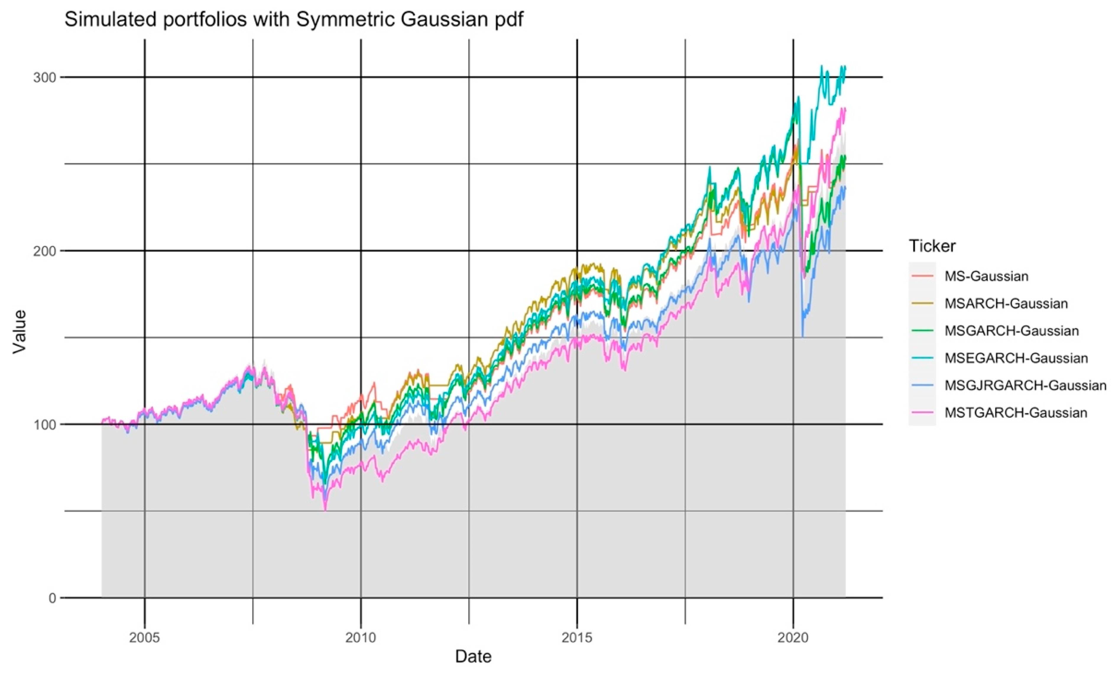
4.1. Simulation Results of the Six Portfolios That Used Homogeneous Symmetric Gaussian pdf

In

Table 3. Performance of the six simulated portfolios that used homogeneous symmetric Gaussian marginal pdfs in the MS-GARCH model log-likelihood function.

Portfolio Performance Metric	MS-Gaussian	MSARCH-Gaussian	MSGARCH-Gaussian	MSEGARCH-Gaussian	MSGJRGARCH-Gaussian	MSTGARCH-Gaussian
Accumulated return	151.8748	152.6977	153.0187	204.0816	135.2070	180.1055
Surplus return from SP500	−15.5524	−14.7295	−14.4085	36.6544	−32.2202	12.6783
Mean return	2.2804	5.1434	5.1616	5.1687	6.1922	4.7622
Return’s std. dev.	0.0383	12.3274	12.1379	16.4089	13.8229	17.3099
Max. drawdown	0.0374	−13.0180	−13.0180	−17.7070	−13.0180	−22.4191
Percentile 2.5%	0.0377	−3.8952	−3.8139	−4.9972	−4.4029	−5.1105
Percentile 97.5%	0.0556	3.1575	3.1360	4.1344	3.6233	4.2425
Sharpe ratio	184.6312	0.5767	0.5872	0.6074	0.4439	0.4988
Jensen’s alpha	151.8748	69.3235	72.1574	56.6335	30.2367	17.3441
Beta with SP500	0	0.4980	0.4830	0.8807	0.6270	0.9721
$R^2$	0	0.4940	0.4793	0.8720	0.6228	0.9548
Tracking error	0.0246	0.0175	0.0178	0.0088	0.0151	0.0053
% of weeks above the SP500	71.3014	70.4116	67.0745	72.6363	44.7164	15.2392
Mean surplus return from the SP500	18.8377	24.2108	20.3116	25.8669	4.6408	5.0846
Mean overperformance	13.4315	17.0472	13.6239	18.7888	2.0752	0.7748
Stock fees paid (total ammount)	20.3046	20.7221	23.4206	22.5830	21.0748	20.1023
Taxes paid (total ammount)	2.0305	2.0722	2.3421	2.2583	2.1075	2.0102

, we summarize the performance of the six simulated portfolios that used a Gaussian pdf (4) as the regime-specific marginal (smoothed, ${\xi }_s,t$) pdf. From the accumulated return and overperformance from the SP500 rows, we show that only the two portfolios that used either asymmetric E-GARCH (Gaussian-EGARCH) or T-GARCH (Gaussian-TGARCH) variances generated an important overperformance at the end of the simulation period. The E-GARCH paid an accumulated return ($PAR$) of 204.08% that was 36.65% higher than the one produced by the SP500. Similarly, the T-GARCH portfolio paid 180.10% of accumulated return (12.67% above the SP500).

Despite this, it was essential to check if this overperformance from the SP500 was a short-term one. To check this, we examined the rows relative to the % of periods above SP500 ($\%weeksup$) and mean overperformance ($MO$), finding that the Gaussian E-GARCH portfolio had a value above the SP500 in 72.63% of the simulated weeks and the T-GARCH had it only in 15.23% of the simulated weeks. In addition, the E-GARCH portfolio had a mean value (surplus) of USD 25.86, leading to a weekly mean overperformance of USD 18.78. That is, on average, this simulated portfolio paid a mean overperformance of USD 18.78 each week. These two results suggest that these two simulated portfolios had a higher value than the SP500 in most weeks.

These results suggest that the use of asymmetric E-GARCH variances was the best to forecast the probability of being in calm ($s=1$) or crisis ($s=2$) regimes or periods, that is, to forecast ${\xi }_{s=1,t+1}$ and ${\xi }_{s=2,t+1}$ to make more precise trading decisions for active portfolio management purposes. We probed this last statement as true with Jensen’s [81] alpha.

This portfolio performance metric measures how much return is due to the portfolio’s manager (the trading algorithm) ability. It was estimated thanks to the portfolios’ beta ($\beta$) with the SP500 as follows:

$$Jense{n}^{\prime }s alpha=PAR-\left[\beta \cdot MAR\right]$$

(19)

As noted in these two best-performing portfolios, the MS-EGARCH portfolio paid 56.63% of its 204.08% accumulated return due to the algorithm’s proper trading sign timing. In plain terms, part of the 204.08% accumulated return was due to market (SP500) performance, given its $\beta =0.8807$ relation with the market, and not by the algorithm’s ability to trade. From that 204.08%, 56.63% was due to the algorithm’s trading timing—timing that generated USD 25.86 mean surplus value from the SP500 during 72.63% of the weeks (a mean weekly overperformance of USD 18.78 from the SP500).

Given this analysis, the best-performing portfolio, from the six portfolios that used the symmetric Gaussian pdf, was the one that used the MS-EGARCH model to forecast the smoothed regime-specific probabilities (${\xi }_{s,t+1}$) at $t+1$.

In Figure 2, we present the historical performance for each simulated portfolio compared against the SP500 (grey area). We present this Figure to give a graphical idea of the performance results in Table 3. The weeks in which the simulated portfolios had a “flat” or horizontal performance were the ones in which the algorithm forecast a high probability (${\xi }_{s=2,t+1}>0.5$) of being in a distress or crisis regime ($s=2$) at $t+1$. Following our trading algorithm’s rule, most simulated portfolios invested in the TBILLs in those periods.

It is interesting to note the impact of the stock trading fees and VAT paid during our simulations. The best-performing portfolio had a 22.58% impact on its performance due to trading fees and 2.25% due to VAT payment.

This result led us to conclude that the impact of stock trading fees and taxes was marginal, related to the net overperformance generated against the SP500.

4.2. Simulation Results of the Six Portfolios That Used Homogeneous Symmetric Student’s t pdf

We follow the same exposition line as for the previous six portfolios. In

Table 4. Performance of the six simulated portfolios that used homogeneous symmetric Student’s t marginal pdfs in the MS-GARCH model log-likelihood function.

Portfolio Performance Metric	MS-tStud	MSARCH-tStud	MSGARCH-tStud	MSEGARCH-tStud	MSGJRGARCH-tStud	MSTGARCH-tStud
Accumulated return	166.8990	74.5301	92.5874	200.9519	140.2742	114.3798
Surplus return from SP500	−0.5282	−92.8971	−74.8398	33.5247	−27.1530	−53.0474
Mean return	2.2804	5.4660	3.1009	3.6491	6.1346	4.8809
Return’s std. dev.	0.0383	11.9015	11.2383	16.5829	14.6248	15.4110
Max. drawdown	0.0374	−13.0180	−13.0180	−22.4191	−13.0180	−22.4191
Percentile 2.5%	0.0377	−3.7158	−3.7158	−4.9211	−4.7248	−4.4590
Percentile 97.5%	0.0556	3.0527	2.9508	3.9675	3.8699	3.9527
Sharpe ratio	206.4728	0.2321	0.3351	0.5906	0.4389	0.3230
Jensen’s alpha	166.8990	−3.0997	23.6568	51.9270	22.5165	−14.6415
Beta with SP500	0	0.4637	0.4117	0.8901	0.7033	0.7706
$R^2$	0	0.4595	0.4063	0.8722	0.7002	0.7569
Tracking error	0.0246	0.0181	0.0190	0.0088	0.0135	0.0121
% of weeks above the SP500	73.1924	42.0467	0	72.6363	31.1457	5.4505
Mean surplus return from the SP500	39.3865	7.1393	0	26.6442	4.6780	1.4422
Mean overperformance	28.8279	3.0018	0	19.3533	1.4570	0.0786
Stock fees paid (total ammount)	21.4620	15.7855	17.6862	22.5111	16.8377	15.7273
Taxes paid (total ammount)	2.1462	1.5785	1.7686	2.2511	1.6838	1.5727

, we summarize the performance of the six portfolios that used a homogeneous Student’s t pdf, as in (5), to filter and smooth the regime-specific probabilities (${\xi }_{s,t}$) at $t$.

The results of these six simulated portfolios are very similar to the symmetric Gaussian pdf ones. The only difference is the fact that only the one that used an MS-EGARCH variance model outperformed the SP500. In this pdf scenario, the T-GARCH portfolio (contrary to its symmetric Gaussian pdf counterpart) did not outperform the SP500.

The E-GARCH portfolio paid a slightly lower accumulated return of 200.95% (against the 204.08% of its symmetric Gaussian pdf counterpart). It had a similar beta of $\beta =0.8901$ with the SP500 and 51.92% of that 200.95% accumulated return was due to the trading algorithm’s ability (Jensen’s alpha). In addition, this E-GARCH simulated portfolio had a higher value than the SP500 in 72.63% of the simulated weeks. This result led to having a weekly mean overperformance of 19.35% against the SP500.

The impact of stock trading fees and VAT was also similar to the one observed in the symmetric Gaussian pdf scenario. The simulated portfolio had an effect of 22.51% due to trading fees and one of 2.25% due to VAT payment.

In Figure 2, we present the historical performance of the six simulated portfolios with a symmetric Student’s t pdf. Similar to Figure 3, the periods in which the simulated portfolios invested in TBILLs show a “flat” performance. In those periods, the simulated portfolios reduced their risk by investing in the TBILL fund due to the forecast probability (${\xi }_{s=2+t1}>0.5$) of being in the crisis regime at $t+1$.

Given the fat tail features of the Student’s t pdf, the simulated E-GARCH portfolio and the time-fixed variance MS one had superior performance, against the SP500, most of the time. In Figure 3, the mean overperformance (USD 39.38) and the proportion of weeks above the SP500 (73.19%) suggest that this underperformance holds in the short-term. In the long term, this portfolio algorithm (MS model with time-fixed variance and Student’s t pdf) significantly outperformed the SP500 and was the most suitable for active portfolio management if the investor assumed a Student’s t pdf.

As noted in Table 4, the impact of stock trading fees and VAT was also marginal (21.46% and 2.14%, respectively), compared with the mean overperformance (39.38%) and the historical performance shown in Figure 2. The use of the Student’s t pdf led to a better performance in crisis episodes such as the October 2008 sub-prime crisis, the 2013 European debt issues, or even the 2020 COVID-19-related market distress.

Given these previous results, using a time-fixed MS variance model led to better performance results (against the SP500) with Student’s t pdf in the regime-specific probabilities ${\xi }_{s,t}$.

4.3. Simulation Results of the Six Portfolios That Used Homogeneous Symmetric GED pdf

Now, we present the result of a fatter-tailed pdf, the generalized error distribution, or GED. Contrary to the Gaussian and, in some $\nu$ values, to the Student’s t pdf, the GED has a polynomial convergence in its tails. That is, the pdf tails are wider and reduce more slowly than the Gaussian and Student’s t pdfs.

In

Table 5. Performance of the six simulated portfolios that used homogeneous symmetric GED marginal pdfs in the MS-GARCH model log-likelihood function.

Portfolio Performance Metric	MS-GED	MSARCH-GED	MSGARCH-GED	MSEGARCH-GED	MSGJRGARCH-GED	MSTGARCH-GED
Accumulated return	143.7509	−8.1618	144.7833	324.4385	144.9373	60.3122
Surplus return from SP500	−23.6763	−175.5890	−22.6440	157.0113	−22.4899	−107.1150
Mean return	2.2804	4.9609	−0.4741	4.9844	8.0490	4.9879
Return’s std. dev.	0.0383	12.1602	15.3636	16.9021	14.4164	16.7758
Max. drawdown	0.0374	−13.0180	−22.4191	−22.4191	−13.0180	−22.4191
Percentile 2.5%	0.0377	−3.8952	−4.7420	−5.1105	−4.7248	−4.9133
Percentile 97.5%	0.0556	3.1117	3.2407	4.1443	3.9527	4.1344
Sharpe ratio	172.8209	−0.1511	0.4341	0.9857	0.4632	0.1175
Jensen’s alpha	143.7509	−89.1989	17.2799	168.4874	30.2932	−92.6573
Beta with SP500	0	0.4840	0.7615	0.9315	0.6847	0.9136
$R^2$	0	0.4796	0.7438	0.9194	0.6829	0.8979
Tracking error	0.0246	0.0178	0.0125	0.0070	0.0139	0.0079
% of weeks above the SP500	70.0779	1.5573	1.6685	72.8587	12.0133	37.9310
Mean surplus return from the SP500	12.4039	4.7431	2.7101	56.9765	1.5361	5.5100
Mean overperformance	8.6924	0.0739	0.0452	41.5123	0.1845	2.0900
Stock fees paid (total ammount)	19.3567	11.4864	18.7296	25.9712	18.8839	15.1649
Taxes paid (total ammount)	1.9357	1.1486	1.8730	2.5971	1.8884	1.5165

, we summarized the performance of the six portfolios that used this symmetric pdf and, in Figure 4, the historical performance of the simulated portfolios.

The conclusions, in this pdf scenario, are similar to the ones of the symmetric Student’s t pdf. The symmetric time-fixed variance MS and the asymmetric E-GARCH variance were the two best performers. Even if the former paid a negative overperformance return against the SP500, the result also held in the short-term.

For the E-GARCH model, it is noted, in Figure 4, an outstanding performance of the simulated portfolio. This result was due to two periods (signaled with black arrows in Figure 4), as mentioned previously, namely, the October 2008 sub-prime financial crisis and the 2013 European debt crisis. Contrary to the other five simulated portfolios, the E-GARCH one sold the SP500 faster and then bought back the SP500 to have another fall in value. Despite this, the proper sell timing in October 2008 and 2013 allowed this portfolio to have a better (higher) accumulated return than the SP500 and the other five simulated portfolios. In addition, as noted in 2013 (the second and third arrows), the simulated portfolio had proper timing to sell and buy back the SP500. This selling activity allowed the portfolio to be liquid less time than the other five and to follow the stock market recovery. This result is noted clearly by the third arrow. As noted, the E-GARCH portfolio spent less time invested in TBILLs because the E-GARCH model, being asymmetric, estimated the leverage effect and rate of converging of past negative and extreme returns.

Related to the week-by-week performance of the E-GARCH portfolio and given a beta of 0.9315 with the SP500, the portfolio active trading strategy (the algorithm) made 168.48% of the 324.43% accumulated return. The return left was due to market movements.

The impact of stock trading fees was 25.97% and the one of VAT was 2.59%. Similar to the previous scenarios, the trade-off between the active accumulated return (169.48%) and the stock trading cost favored the use of our algorithm with an MS-EGARCH model.

With the results summarized in Figure 4 and Table 5, we conclude that the best-performing portfolio in a GED pdf context was the one that used an asymmetric MS-EGARCH model.

Given the above presentation of our results with symmetric pdfs, we now show the ones of the three asymmetric (Fernández–Steel skewed) probability functions.

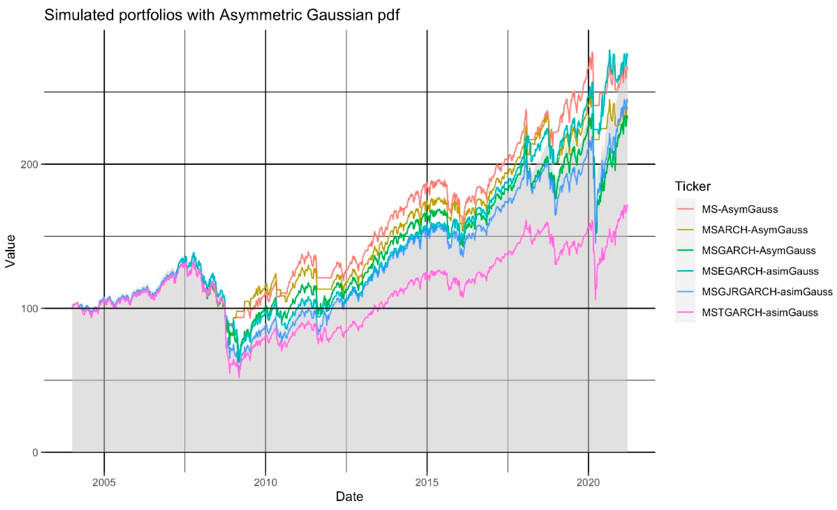
4.4. Simulation Results of the Six Portfolios That Used Homogeneous Asymmetric Gaussian pdf

In

Table 6. Performance of the six simulated portfolios that used homogeneous asymmetric Gaussian marginal pdfs in the MS-GARCH model log-likelihood function.

Portfolio Performance Metric	MS-AsymGauss	MSARCH-AsymGauss	MSGARCH-AsymGauss	MSEGARCH-AsimGauss	MSGJRGARCH-AsimGauss	MSTGARCH-AsimGauss
Accumulated return	165.8868	138.2622	131.9116	174.7129	143.1381	70.4097
Surplus return from SP500	−1.5404	−29.1650	−35.5156	7.2857	−24.2891	−97.0175
Mean return	2.2804	5.4449	4.8341	4.6837	5.6267	4.9469
Return’s std. dev.	0.0383	12.2538	12.2414	16.5886	13.9874	17.4269
Max. drawdown	0.0374	−13.0180	−13.0180	−17.7070	−13.0180	−22.4191
Percentile 2.5%	0.0377	−3.8139	−3.8952	−5.1105	−4.6889	−4.9979
Percentile 97.5%	0.0556	3.1360	3.1575	4.1344	3.6406	4.2425
Sharpe ratio	205.0013	0.5146	0.4863	0.5024	0.4703	0.1453
Jensen’s alpha	165.8868	55.9083	49.7632	23.8347	35.7985	−94.8680
Beta with SP500	0	0.4919	0.4907	0.9012	0.6411	0.9872
$R^2$	0	0.4878	0.4863	0.8934	0.6360	0.9714
Tracking error	0.0246	0.0176	0.0176	0.0080	0.0148	0.0042
% of weeks above the SP500	71.9689	70.3003	54.6162	75.0834	8.1201	0.3337
Mean surplus return from the SP500	25.1829	16.3290	7.5454	6.9984	0.7145	0
Mean overperformance	18.1239	11.4793	4.1210	5.2546	0.0580	0
Stock fees paid (total ammount)	20.9520	19.7624	21.6777	21.0115	20.5856	16.9013
Taxes paid (total ammount)	2.0952	1.9762	2.1678	2.1012	2.0586	1.6901

and Figure 5, we summarize the performance of the six portfolios that used an asymmetric Gaussian pdf.

As noted, the results are similar to the ones of the symmetric Gaussian scenario, in which the time-fixed MS and the MS-EGARCH portfolios were the best performers. The MS-EGARCH portfolio had an overperformance of 7.28%, a result explained with a weekly mean overperformance of USD 5.25. This average overperformance was considerably lower than the one observed in the symmetric Gaussian pdf scenario. In addition, the accumulated return of 7.28% was lower than the 33.52% paid by the symmetric Gaussian MS-EGARCH portfolio.

Figure 5 and the beta value of this MS-EGARCH portfolio (Table 6) show that this portfolio had a performance close to the SP500. Given this, the use of an asymmetric Gaussian pdf did not add value to our trading strategy compared with the symmetric Gaussian case.

Departing from this result, the use of MS-EGARCH models with asymmetric Gaussian pdfs was the best option in this scenario, but still, using an asymmetric Gaussian pdf was not better than using a symmetric one.

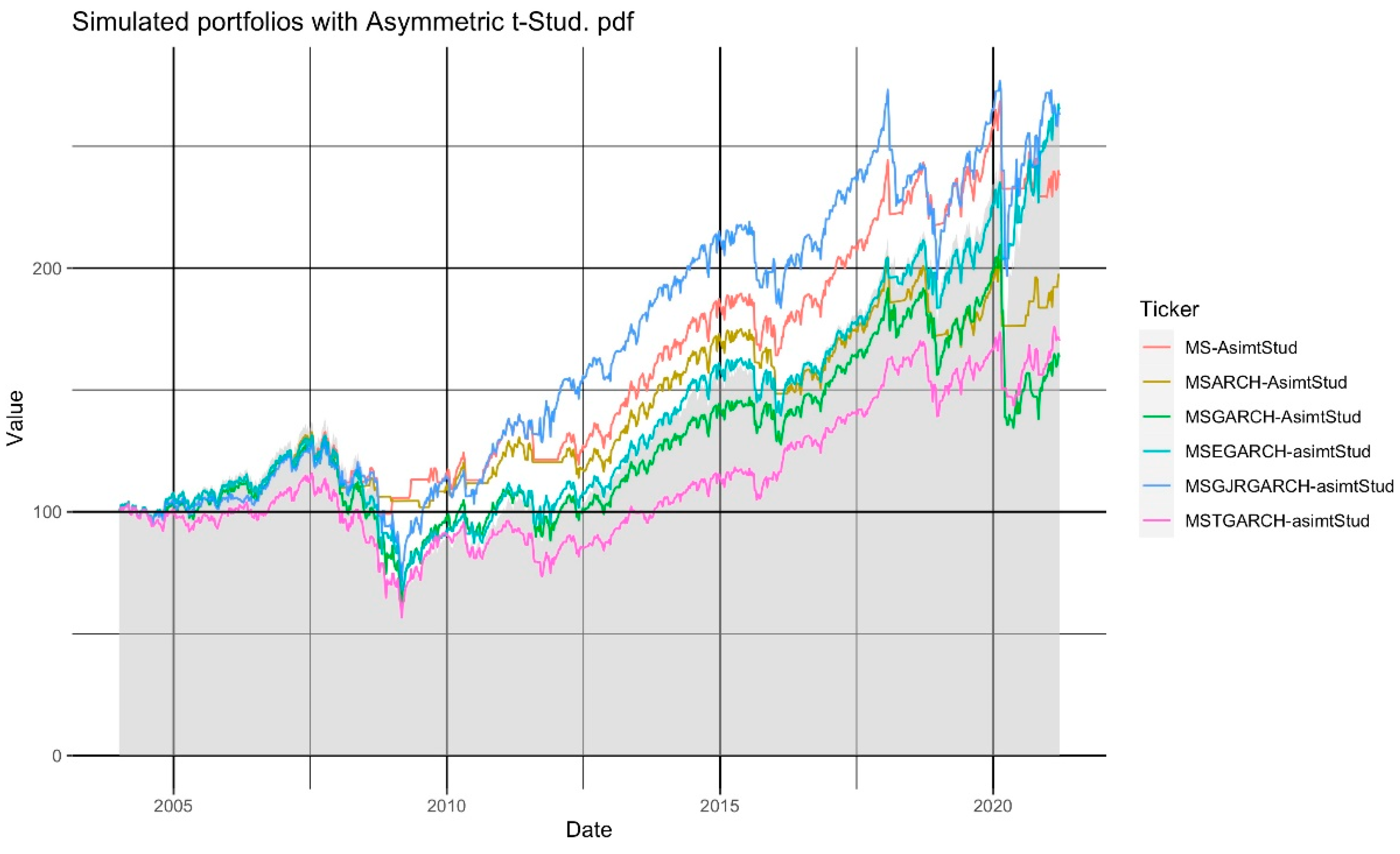
4.5. Simulation Results of the Six Portfolios That Used Homogeneous Asymmetric Student’s t pdf

In

Table 7. Performance of the six simulated portfolios that used homogeneous asymmetric Student’s t marginal pdfs in the MS-GARCH model log-likelihood function.

Portfolio Performance Metric	MS-AsimtStud	MSARCH-AsimtStud	MSGARCH-AsimtStud	MSEGARCH-AsimtStud	MSGJRGARCH-AsimtStud	MSTGARCH-AsimtStud
Accumulated return	137.9941	97.2645	63.5761	165.0751	162.9193	70.2109
Surplus return from SP500	−29.4331	−70.1627	−103.8511	−2.3521	−4.5079	−97.2163
Mean return	2.2804	4.8278	3.7827	2.7400	5.4279	5.3824
Return’s Std. dev.	0.0383	11.7953	10.6905	16.2467	14.4487	15.1295
Max. drawdown	0.0374	−13.0180	−13.0180	−17.7070	−13.0180	−17.7070
Percentile 2.5%	0.0377	−3.8139	−3.5697	−5.1105	−4.7248	−4.8769
Percentile 97.5%	0.0556	3.0314	2.9870	4.1318	3.8387	3.9527
Sharpe ratio	164.4519	0.3413	0.2014	0.4800	0.5314	0.1667
Jensen’s alpha	137.9941	21.1045	0.8981	20.7684	48.1425	−55.2063
Beta with SP500	0	0.4549	0.3744	0.8619	0.6855	0.7491
$R^2$	0	0.4502	0.3712	0.8520	0.6815	0.7421
Tracking error	0.0246	0.0182	0.0195	0.0095	0.0139	0.0125
% of weeks above the SP500	72.1913	45.0501	18.0200	49.7219	73.3037	6.7853
Mean surplus return from SP500	26.0740	18.4318	6.2985	4.3217	38.4856	1.6287
Mean overperformance	18.8232	8.3035	1.1350	2.1488	28.2114	0.1105
Stock fees paid (total ammount)	20.0073	16.3535	18.3685	19.9733	21.2226	14.8509
Taxes paid (total ammount)	2.0007	1.6353	1.8368	1.9973	2.1223	1.4851

and Figure 6, we present the portfolios’ performances that used an asymmetric Student’s t pdf. As noted in Table 7, all the simulated portfolios showed underperformance—an underperformance that held in the short-term (in the last weeks only).

Despite this, two portfolios showed an important overperformance against the SP500. These are the portfolio that used a time-fixed variance MS mode and the asymmetric GJR-GARCH one. From these two, the latter is the one that showed a significantly better performance than the SP500 by having a higher value than this index in 73.30% of the simulated weeks and a weekly mean overperformance of USD 28.21 (the highest observed one in these portfolios). As noted with the 0.6855 SP500 beta value and the 48.15% Jensen’s alpha, this portfolio added 48.14% of active return given the use of the trading algorithm with asymmetric Student’s t pdf and an MS-GJRGARCH model. As in the previous scenarios, 48.14% of the 162.91% of accumulated return was due to the algorithm’s timing, given the forecast regime-specific probabilities ${\xi }_{s,t+1}$.

As is the case of the four previous pdf scenarios, the impact of stock trading fees and taxes was marginal (21.22% and 2.12%, respectively).

4.6. Simulation Results of the Six Portfolios That Used Homogeneous Asymmetric GED pdf

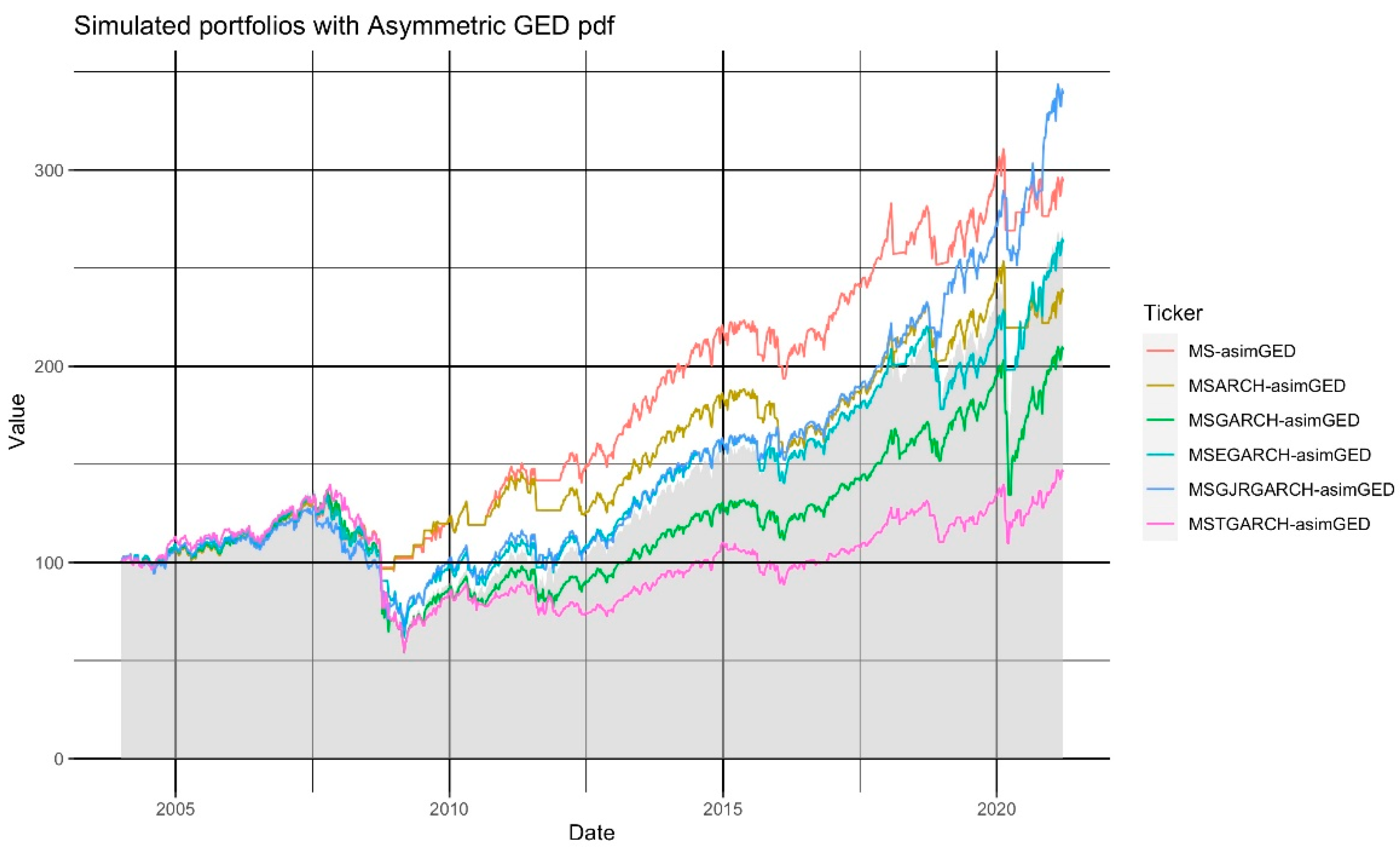
Finally, we present the results of the six simulated portfolios that used an asymmetric GED pdf. In

Table 8. Performance of the six simulated portfolios that used homogeneous asymmetric GED marginal pdfs in the MS-GARCH model log-likelihood function.

Portfolio Performance Metric	MS-AsimGED	MSARCH-AsimGED	MSGARCH-AsimGED	MSEGARCH-AsimGED	MSGJRGARCH-AsimGED	MSTGARCH-AsimGED
Accumulated return	193.9386	137.6817	108.2635	163.0244	238.4980	46.0118
Surplus return from SP500	26.5114	−29.7455	−59.1637	−4.4028	71.0708	−121.4154
Mean return	2.2804	6.0033	4.8205	4.0848	5.3846	6.7892
Return’s std. dev.	0.0383	11.8502	11.8181	17.0938	14.4377	14.1813
Max. drawdown	0.0374	−13.0180	−13.0180	−22.4191	−13.0180	−10.4738
Percentile 2.5%	0.0377	−3.7158	−3.7158	−4.9231	−4.7248	−4.4590
Percentile 97.5%	0.0556	3.0879	3.0527	4.1284	3.6854	3.8783
Sharpe ratio	245.7820	0.5295	0.3924	0.4495	0.8229	0.0829
Jensen’s alpha	193.9386	60.5480	31.7420	4.3452	123.9510	−65.0741
Beta with SP500	0	0.4607	0.4570	0.9478	0.6842	0.6635
$R^2$	0	0.4575	0.4528	0.9306	0.6798	0.6626
Tracking error	0.0246	0.0181	0.0182	0.0065	0.0139	0.0143
% of weeks above the SP500	74.3048	70.4116	1.0011	63.2925	77.8643	17.7976
Mean surplus return from the SP500	50.1670	21.4593	0.0499	4.6337	15.4081	3.1757
Mean overperformance	37.2765	15.1098	0.0005	2.9328	11.9974	0.5652
Stock fees paid (total ammount)	22.9403	19.3979	18.0753	20.0089	20.8130	13.2900
Taxes paid (total ammount)	2.2940	1.9398	1.8075	2.0009	2.0813	1.3290

and Figure 7, we summarize the results. Only the portfolios that used a time-fixed variance (MS) or a GJR-GARCH one led to an overperformance against the SP500. In the MS portfolio, we found a 26.51% extra return from the SP500 and, in the GJR-GARCH, an extra return of 71.07%. The former had a higher value than the SP500 in 74.30% of the weeks from these two simulated portfolios, while the latter, had a higher value of the SP500 in 73.30% of the weeks. The trading algorithm with these pdfs and variance models led to a mean overperformance, against the SP500, of USD 18.82 and USD 28.21, respectively.

By inspecting the historical performance of these two portfolios in Figure 7, the MS model had an important overperformance in most simulation periods. The benefits of the GJR-GARCH one could be seen only at the end of our simulations. Given this and despite the mean overperformance of the GJR-GARCH portfolio, we prefer to consider the time-fixed variance MS model as the best one in the asymmetric GED scenario.

4.7. Corollary of Results of the Six Simulated pdf Scenarios

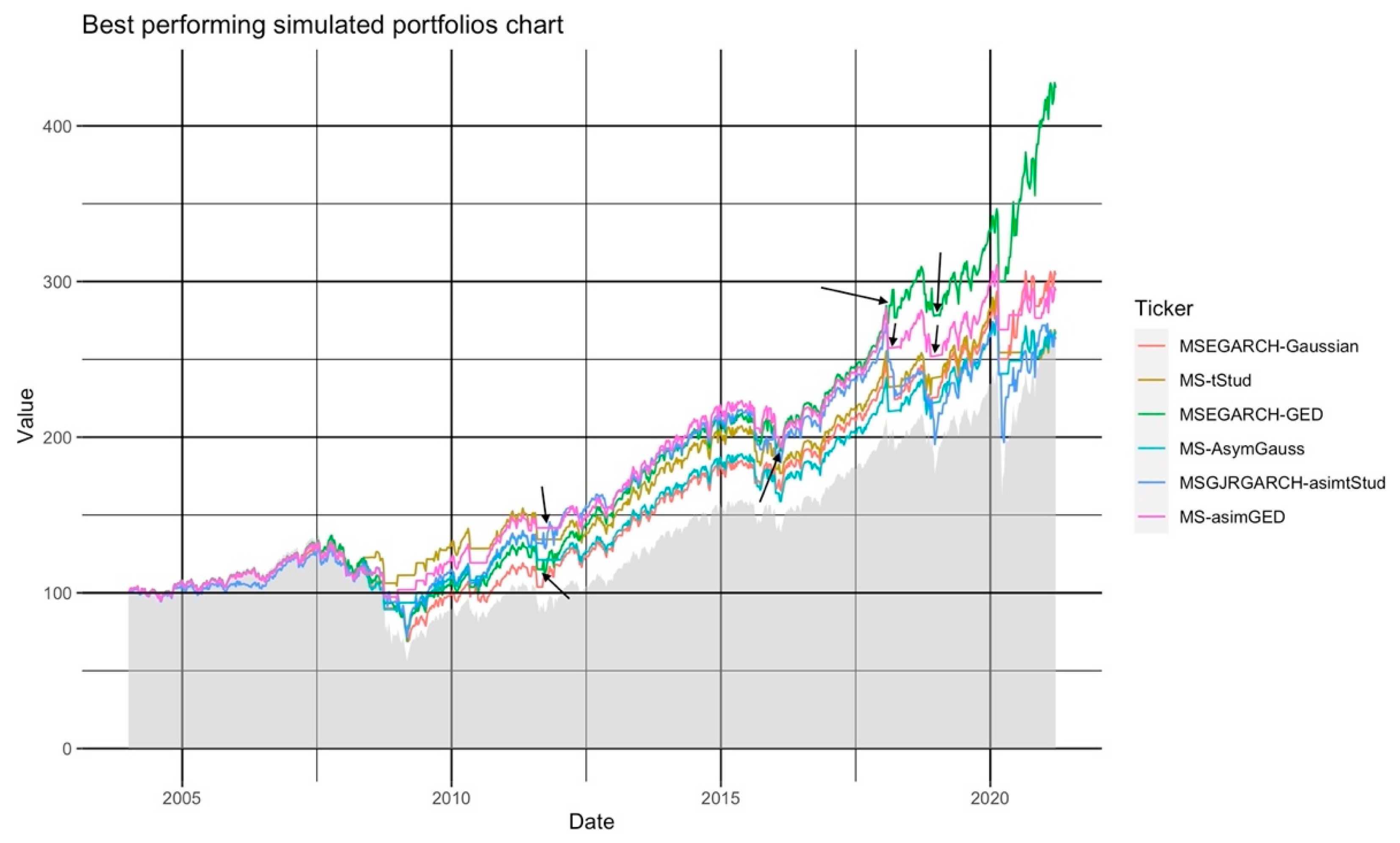
In

Table 9. Performance of the best-performing portfolios in the six pdf-specific analyses made in the previous sub-sections.

Portfolio Performance Metric	MSEGARCH-Gaussian	MS-tStud	MSEGARCH-GED	MS-AsymGauss	MSGJRGARCH-AsimtStud	MS-AsimGED
Accumulated return	204.082	166.899	324.438	165.887	162.919	193.939
Surplus return from SP500	36.654	−0.528	157.011	−1.540	−4.508	26.511
Mean return	5.169	2.280	4.984	2.280	5.428	2.280
Return’s std. dev.	16.409	0.038	16.902	0.038	14.449	0.038
Max. drawdown	−17.707	0.037	−22.419	0.037	−13.018	0.037
Percentile 2.5%	−4.997	0.038	−5.111	0.038	−4.725	0.038
Percentile 97.5%	4.134	0.056	4.144	0.056	3.839	0.056
Sharpe ratio	0.607	206.473	0.986	205.001	0.531	245.782
Jensen’s alpha	56.634	166.899	168.487	165.887	48.142	193.939
Beta with SP500	0.881	0	0.932	0	0.686	0
$R^2$	0.872	0	0.919	0	0.682	0
Tracking error	0.009	0.025	0.007	0.025	0.014	0.025
% of weeks above the SP500	72.636	73.192	72.859	71.969	73.304	74.305
Mean surplus return from the SP500	25.867	39.386	56.977	25.183	38.486	50.167
Mean overperformance	18.789	28.828	41.512	18.124	28.211	37.276
Stock fees paid (total ammount)	22.583	21.462	25.971	20.952	21.223	22.940
Taxes paid (total ammount)	2.258	2.146	2.597	2.095	2.122	2.294

and Figure 8, we summarize the six best-performing portfolios of each of the previous pdf-specific analyses. By following the last analysis, we found that the best-performing variance model and pdf for the LLF and regime-specific probabilities (${\xi }_{s,t}$) was the one with symmetric GED pdf and an E-GARCH variance, that is, to use a GED MS-EGARCH to forecast the regime-specific probabilities (${\xi }_{s,t+1}$).

These results could help an institutional investor, such as an ETF or a mutual fund, to perform an active portfolio strategy to buy the SP500 index in calm periods (s = 1) and sell it in crisis or distress ($s=2$).

Using the suggested algorithm with a GED MS-EGARCH, an investor could have a mean weekly USD 41.51 value above the SP500 because their fund would be above this index in 72.85% of the weeks. This result is due to proper timing in the trading signals given with the algorithm and is marked by the green line in Figure 8.

Another best-performing MS model was the time-fixed variance MS-GED model (pink line in Figure 8). Despite its good performance most of the time, the time-fixed variance led this simulated algorithm to invest in TBILLs more often than the GED MS-EGARCH one, which is an issue that did not happen with the GED MS-EGARCH portfolio. This last portfolio correctly identified the beginning of high-volatility periods with adverse return movements (given the leverage effect of the negative returns in the EGARCH variance model). It reinvested its proceeding in the SP500 when the variance was lower. These trading decisions led this portfolio to lose some of the SP500 price recoveries identified as “high-volatility” periods. Figure 8 highlights the weeks in which the symmetric GED-MSEGARCH model led to more precise trading signs than the asymmetric GED-MS one.

Given these results, the best combination of pdf and variance for active trading in the SP500 with the suggested algorithm was the one that used a symmetric fat-tailed GED pdf and an asymmetric variance model such as the E-GARCH.

Furthermore, as mentioned in Section 4.3, the impact of stock trading fees and taxes was marginal (21.46% and 2.14%, respectively) in the accumulated return.

In terms of alpha generation, we found that using the MS-EGARCH model led to 168.48% of the 324.43% of accumulated return. In total, 51.93% of that accumulated return was due to the trading signs of the suggested MS-EGARCH algorithm; the other 48.06% was due to market movements.

4.8. The Performance of the Simulated Portfolios in Extraordinary High-Volatility Periods

There is a particular feature that we mention in the above review that we want to briefly highlight in this subsection, i.e., the performance of the best-performing portfolios in each of the six pdf or log-likelihood function (LLF) scenarios. Reviewing Figure 3, Figure 4, Figure 5, Figure 6, Figure 7 and Figure 8, it can be noted that the simulated algorithm worked appropriately in almost all the high-volatility periods. In periods such as the 2007–2008 sub-prime crisis, it can be observed that the algorithm made an accurate forecast of the distress period. The best-performing portfolio (with an asymmetric GED MS-EGARCH model) sold the risky asset (the SP500 fund) and avoided this crisis episode correctly.

Despite this timing improvement, the algorithm, given its parameters, has two drawbacks. First, there are stock market downward movements with a volatility level (lower than previous regimes, such as the 2013 European debt crisis); given this, there is a possibility that the MS-GARCH scale-only estimation method cannot prevent downward trends. Second, we assumed a two-regime context for the algorithm; departing from this assumption, extreme volatility episodes (such as the 2020 COVID-19 crisis) can be forecast with lags. That is, the two-regime MS-GARCH model could trigger a sell signal once the high-volatility regime starts and not before that moment.

Despite these two drawbacks, the algorithm is still helpful for the active trading purposes tested herein. As a potential guideline for further research, we could suggest using a three-regime context or even using a sequential regime and market trend algorithm, such as the one by Hauptman et al. [34] or Engel et al. [35]. In addition, the use of other MS-GARCH estimation methods with neural networks (such as in Liao, Yamaka and Sriboonchitta [43]) could be a potential solution.

4.9. Feasibility in Terms of Algorithm Execution and Implementation

The previous results show how useful MS-GARCH models would be in forecasting changes in US stock market regimes. As mentioned previously, these regimes are a proxy of stock market agents’ behavior and their accurate forecast at $t+1$ could give an advantage to investors to buy (sell) a stock market portfolio (such as the SP500) in forecast low- (or high-) volatility periods.

A final practical question remains, i.e., is it feasible for an institutional or private investor to implement our simulation algorithm? The answer is yes. We made our simulations on a Mac Pro with a six-core 3.5 GHz Intel Xeon E6 processor, 18 GB of RAM and an AMD Fire pro D500 3G graphic processor. In the macOS Catalina operative system, we used Ardia et al.’s [76] MSGARCH library in R.

The library and the R programming language are licensed under the creative commons license for almost all the operative systems. Such software can be installed in a server with Devian for public access on an intranet or a cloud service.

To store all the data of each model in each simulation, we used an SQLite file. In one data table, we stored the historical SP500 price data and, in another one, the results of our MS-GARCH model estimations. In a third table, we simulated the performance of the 36 portfolios of interest. We used the MariaDB file to have faster access to all the backtest.

The estimation of each of the 36 MS-GARCH models had a mean duration of 41.54 s each week. The two models that took longer in their estimate were the symmetric GED MS-GJRGARCH and MS-TGARCH models in the last week of our simulations (4863 weeks of historical data in the information set). We estimated the former in 76.43 s and the latter in 76.79 s. In Appendix A, we present, in detail, the estimation times of each of the 36 models during our simulations. It is essential to mention that these estimation times include other data analysis processes, such as estimating the continuous-time returns of the SP500.

If an analyst wanted to estimate the 36 models, she or he would need, at most, only 38.16 min at the end of each week. They would also need 3 min, at most, to determine the best fitting MS-GARCH model and to obtain a final trading decision.

It is essential to mention that the estimation times depend on the computer capabilities and the default settings used, such as the number of MCMC paths estimated (10,000) or the value of the starting seed for the estimation methods. Despite this warning, the model can be implemented on a PC or cloud service and even used for algorithmic trading purposes.

We show that it is feasible to implement our suggested trading algorithm in daily or even intraday periods from these simulation times. Despite these research recommendations, we suggest extending our tests to intraday periods as guidelines for further research. It is important to note that the use of MS-GARCH, the number of regimes and their behavior could change in smaller periods than daily or weekly.

5. Conclusions

The use of Markov-switching with generalized autoregressive conditional heteroskedasticity (MS-GARCH) models in stock trading algorithms could be a potential solution to enhance the performance of equity funds or ETFs by forecasting the probability (${\xi }_{s=2,t+1}$) of being in a distressing period. With this forecast, an investor could determine if it is appropriate to sell stocks, buy a risk-free asset in distress periods, or do the opposite in calm ones.

This proposal is not a novelty and started with Brooks and Persand [29], who tested the use of time-fixed variance Markov-switching (MS) models as a potential tool to reduce noise and uncertainty in investors’ decisions. Despite this, there has been little discussion about the benefits of such a strategy and similar algorithmic trading applications.

Departing from the behavioral finance rationale that noisy traders tend to create bubbles or crashes due to the use of sentiments in their decisions, a quantitative tool to forecast the market crisis or high-volatility periods is of interest to us.

The present paper extends the literature by testing the benefit of asymmetric probability density functions (pdf) and asymmetric GARCH variance models in a two-regime trading algorithm in the US S&P 500 stock index (SP500).

Our position is that asymmetric models could lead to better trading signs because there are well-documented asymmetries in the performance of stock returns.

With weekly data of the SP500 from 6 January 1928 to 19 March 2021, we simulated (from 2 January 2004 to 19 March 2021) the performance that an institutional investor would have had, had they used a trading algorithm with the following trading rules:

• To invest in the SP500 if the probability of being in low-volatility, calm or “normal” ($s=1$) periods at $t+1$ is higher than 50% (${\xi }_{s=1,t+1}>0.5$).
• To invest in the US risk-free asset (TBILL) if the probability of being in high-volatility, distress, or “crisis” ($s=2$) periods at $t+1$ is higher than 50% (${\xi }_{s=2,t+1}>0.5$).

Our position is that the use of either asymmetric pdf or asymmetric GARCH models (such as the EGARCH) could enhance the portfolio’s performance against the SP500 and the portfolios that used either a symmetric pdf or variance model.

We simulated the performance of 36 theoretical portfolios (6 portfolios with different MS-GARCH models for the symmetric or asymmetric Gaussian, Student’s t, or generalized error distribution—GED—pdf). Our results show that the portfolio that used a symmetric GED pdf and an asymmetric EGARCH variance (MS-EGARCH) model performed best.

From the 36 simulated portfolios, this was the one that outperformed the SP500 most of the time (72.85% of the time). This result led to a weekly mean overperformance of USD 41.52 (from a USD 100 base value) above this index. Given this, the simulated portfolio paid an accumulated return of 324.43% (157.01% more than the SP500). From this accumulated return, 168.48% was due to the proper timing in the trading decisions (buy or sell the SP500). In a trading costs–performance trade-off analysis, we found that using weekly rebalancing led to a 25.97% impact due to stock trading fees and a 2.59% impact due to taxes.

Our results, obtained by testing, contribute to the discussion about the benefits of using MS-GARCH models in trading algorithms by showing that the best combination of pdf and variance model for trading US stocks is to use a symmetric GED pdf and an E-GARCH variance model in the Markov-switching model. This last model with this configuration led to more precise forecasts of the regime-specific probabilities (${\xi }_{s,t+1}$). These forecasts allowed us to determine the probability of being in a high-volatility or distress regime at $t+1$. Given these forecasts, the simulated trading algorithm led to better trading signs and better performance than a buy-and-hold strategy in the SP500 index.

In a theoretical financial economics context, our results add to the discussion about the balance of informed and noisy traders in the markets. An issue in the current behavioral financial economics testing is that market crashes or bubble episodes are ascribed to the not-so-rational behavior of noisy traders. Similar to the one tested herein, an MS-GARCH trading algorithm could be helpful to sort the changes in volatility regimes, due to market sentiment change, in the financial market.

Institutional investors such as mutual funds or exchange-traded funds could use an algorithm such as the one tested herein by knowing that a symmetric, fat-tailed and polynomial GED log-likelihood function (LLF) with an asymmetric E-GARCH variance model is the best MS-GARCH model for investment decisions. The fat-tailed pdf could incorporate the odds of having extreme values in each regime. The E-GARCH, as noted in our results, could help enhance the timing of selling the SP500 in distress periods and repurchase it with a proper low-volatility regime forecast at $t+1$. The leverage effect (a higher weight of negative returns) of the E-GARCH variance in each regime enhanced the prediction power of the MS-EGARCH model.

Our results are part of several tests to enhance Markov-switching models and the trading algorithms with these. Despite this, we believe there is room to extend our results. First, we suggest repeating our tests of the 36 simulated portfolios and comparing their results with MS-GARCH models with heterogeneous pdf in the LLF and heterogeneous variance (time-fixed or GARCH) models, using different pdf and GARCH models in each regime and not homogeneous ones, as we show here. This guideline is hard in computational terms because of the number of combinations of symmetric or asymmetric pdf and GARCH variances. This guideline implies the extension of using either symmetric or asymmetric pdfs and variance models.

Another extension of our tests would be using other assets in the high-volatility regime, such as volatility futures, another type of negatively related security, or even the performance of short selling.

In addition, to test the use of MS-GARCH models with three or more regimes could be of interest in terms of financial econometrics, active portfolio trading, algorithmic trading and investment management.

The use of other periodicities in the test (such as daily or even intraday ones) or other estimation methods different from Markov chain Monte Carlo (MCMC) could be of interest. Some suggestions could be the use of neural networks [43] or other deep learning techniques.