On the τ Decomposition Method for the Stability and Bifurcation of the TCP/AQM Networks versus Time Delay

Abstract

This paper investigates the nonlinear dynamics of Transmission Control Protocol and Active Queue Management (TCP/AQM) networks, including the local stability and periodic bifurcation. The parameter of transportation delay affects the stability of the dynamical systems. One of the purposes of our work is to determine the delay stable interval of the transportation network. It is found that there is only one critical value of network delay by the $\tau$ decomposition technique. When the delay passes the critical point, the system performs Hopf bifurcation with a pair of symmetry with purely imaginary roots (PIR). In addition, the other purpose is to consider the stability of bifurcating periodic solutions. Combining with $\tau$-decomposition strategy and central manifold theory, the issues of delay stable interval and stability of Hopf bifurcation are all tackled. Finally, numerical examples are illustrated to show the accuracy and effectiveness of the proposed method.

1. Introduction

With an increasing number of network devices in life, the quality of Internet communication becomes more important. The Internet will become crowded and the quality of Internet communication will seriously decline when there is too much data. Generally, the function of congestion control algorithm is that it will eventually avoid congestion through returning congested information to the data sender, who can adjust the rate of data transmission. The congestion control algorithm is largely dependent on the TCP/AQM mechanism.

As far as the authors’ concerns, a practical nonlinear network model is proposed in [1,2,3], associating with the proportional feedback and the delay feedback strategies. In addition, the local asymptotic stability around the system’s equilibrium point is addressed. There is no doubt that the dynamics of systems with time delay become more complex than the ordinary ones. Thus, a lot of attention is given to the analysis of nonlinear dynamics for the TCP/AQM networks with transport delay. In addition, substantial achievements are obtained by the scholars. By using the Lyapunov–Krasovskii functional approach, the sufficient stability conditions are derived for a class of nonlinear time delay systems encountered as fluid network models in [4]. In [5], Yang and Tian consider the exhibition of Hopf bifurcation for an Internet congestion control algorithm with communication delay. In addition, the formulas for calculating the direction and stability of bifurcation solutions are proposed. Combined with analytical and numerical tools, the linear stability, bifurcation, and chaos of the TCP/AQM network with time delay are considered in [6]. Zheng and Nelson developed an $H_{\infty }$ approach to design an active queue management (AQM) for wireless networks with communication delay. In [7], the linear stability and the bifurcation are considered for the network model with the exponential Random Early Detection (RED) algorithm, with the characteristic equation method and center manifold theory. Meanwhile, some classes of nonlinear fluid flow models with internet congestion control algorithm are investigated in [8], by using control and bifurcation theories. In [9], the local stability of the equilibrium of system with the exponential RED algorithm and heterogeneous delays is tackled by applying generalized Nyquist criteria. Zheng and Wang investigated the local dynamics of a class of TCP/AQM networks with proportional feedback and communication delay. In addition, the periodic motion of the bifurcation examines the method of multiple scales in [10]. Moreover, the bifurcation behaviors of internet congestion control system with the eXplicit Control Protocol (XCP) and delayed feedback are determined in [11]. The local dynamics of FAST TCP model with internet congestion control algorithms are addressed in [12]. Both of the necessary and sufficient stability conditions and determination of bifurcating solutions are obtained. Recently, a new TCP/AQM system is proposed to improve the accuracy of the MGT fluid model in [13]. Both of the discrete and continuous time models are provided. More recently, complex dynamics of transmission control protocol network with transmission delay and wireless access links and packet error rate (PER) have been investigated in [14]. It is noted that different TCP or the buffer sizes lead to different queuing regimes and models. More complex analysis on large nonlinear models is provided in [15,16,17].

Indeed, both of the analysis tools and the control algorithms are benefits for analyzing the dynamical behaviors of the TCP/AQM networks with delays. However, the unified framework for the determinations of the local and bifurcation dynamics is still necessary. Under the factors described above, we provide a practical and systematic procedure to test the nonlinear dynamics of the TCP/AQM model. Some general stability criteria involving the delays are derived. The uniqueness of delay stable interval is given. In addition, the endpoint can be computed analytically. By choosing the delay as a bifurcation parameter, it is shown that the system performs Hopf bifurcation on the endpoint, i.e., the critical delay. Finally, a concise algorithm is provided for the determination of the directions and stability of the bifurcation solutions.

2. Problems Statement and Preliminaries

Due to the symmetry of conjugate complex roots, only positive pure imaginary roots are considered in the subsequent analysis. The TCP/AQM network dynamic model is described as the following nonlinear differential equation:

$$\begin{array}{c}\dot{W}\left(t\right)=\frac{1}{R\left(t\right)}-\frac{W\left(t\right)W(t-R(t\left)\right)}{2R(t-R(t\left)\right)}p(t-R\left(t\right))\hfill \\ \dot{Q}\left(t\right)=N\left(t\right)\frac{W\left(t\right)}{R\left(t\right)}-C\hfill \end{array}$$

(1)

where $W\left(t\right)$ indicates the average TCP window size (packets), $Q\left(t\right)$ indicates the average queue length (packets), $R\left(t\right)$ indicates the round trip time (seconds), C indicates the network queue capacity (packets/second), $N\left(t\right)$ indicates the number of TCP sessions, and $p(·)$ indicates the probability function of packet markers. Queue length $Q\left(t\right)$ and window size $W\left(t\right)$ are positive.

In this paper, $p\left(t\right)$ is proportional to $Q\left(t\right)$, that is, $p\left(t\right)=KQ\left(t\right)$. Moreover, the value of network capacitance C is large, and assume that the number of TCP streams $N\left(t\right)$ remains unchanged. The propagation delay determines the value of $R\left(t\right)$, which is treated as a constant R in our discussion. Equation (1) can be transformed into:

$$\begin{array}{c}\dot{W}\left(t\right)=\frac{1}{R}-\frac{W\left(t\right)W(t-R)}{2R}KQ(t-R)\hfill \\ \dot{Q}\left(t\right)=N\left(t\right)\frac{W\left(t\right)}{R}-C\hfill \end{array}$$

(2)

In addition, it is easy to verify that Equation (2) has a unique equilibrium point $(We,Qe)$, with

$$W_e=\frac{CR}{N},Q_e=\frac{2N^2}{K{C}^2{R}^2}.$$

By introducing two new variables, $w\left(t\right)=W\left(t\right)-W_e,q\left(t\right)=Q\left(t\right)-Q_e$, Equation (2) becomes:

$$\begin{array}{c}\dot{w}\left(t\right)=\alpha w\left(t\right)+\alpha w(t-R)+\beta q(t-R)+w_f\hfill \\ \dot{q}\left(t\right)=\gamma w\left(t\right)\hfill \end{array}$$

(3)

with $w_f=\mu w\left(t\right)w(t-R)\nu [w\left(t\right)+w(t-R)]q(t-R)+\rho w\left(t\right)w(t-R)q(t-R)$ and

$$\begin{array}{c}\alpha =-\frac{N}{C{R}^2},\beta =-\frac{KR{C}^2}{2N^2},\gamma =\frac{N}{R},\hfill \\ \mu =-\frac{N^2}{C^2{R}^3},\nu =-\frac{CK}{2N},\rho =-\frac{K}{2R}.\hfill \end{array}$$

It is clear that Equation (3) is a model established on the basis of Equation (2) with equilibrium point as the origin.

Generally speaking, we consider the linear stability and the Hopf bifurcation versus feedback delay for the TCP/AQM system in (3). The linearization of system (3) is necessary for the issues of local stability, and we have the following matrix form linear part of (3)

$$\dot{x}=Ax\left(t\right)+Bx(t-R)$$

(4)

with

$$A=\left[\begin{array}{cc}\alpha & 0\\ \gamma & 0\end{array}\right],B=\left[\begin{array}{cc}\alpha & \beta \\ 0& 0\end{array}\right]\mathrm{and}x\left(t\right)=\left[\begin{array}{c}w\left(t\right)\\ q\left(t\right)\end{array}\right]$$

(5)

It easy to verify that the corresponding characteristic equation of (4) is

$$P(R,\lambda )=det(\lambda I-A-B{e}^{-R\lambda })={\lambda }^2-\alpha \lambda -(\alpha \lambda +\beta \gamma )e^{-R\lambda }$$

(6)

Before we proceed, some necessary assumption should be introduced to exclude the unstable case.

Assumption 1.

It is assumed that $\alpha <0$ and $\beta \gamma <0$. Otherwise, the systems (4) cannot be stable for any $\tau \ge 0$.

As is indicated in [18], the $\tau$ decomposition method mainly related to two aspects of works: the computation of purely imaginary roots (PIR) and the cross direction over the PIRs. For the first part of the work, since the conjugate complex roots are symmetry with respect to the real axis, we only need to consider the positive pure imaginary roots. We follow the line of [19] and have

Proposition 1.

The transcendental Equation (6) has only one purely imaginary root (PIR), such that

$${\omega }_0=\sqrt{{\beta }^2{\gamma }^2}$$

(7)

On the other hand, the cross direction around $j{\omega }_0$ is always to the right, which is addressed in [20], clearly. Therefore, as for the local stability of system in (2), it is stated below.

Theorem 1.

The equilibrium $(W_e,Q_e)$ of system (2) is exponentially stable for $R\in [0,R_0)$, and it is unstable for $R\in [R_0,+\infty )$, with

$$R_0=\frac{{\theta }_0+\pi }{{\omega }_0}$$

(8)

in which ${\theta }_0=\angle \frac{-{\omega }_0^2+\alpha {\omega }_{0}j}{{\omega }_0^2+\alpha {\omega }_{0}j}$, $\angle (·)$ stands for “argument of a complex number”. Moreover, $R_0$ is a Hopf bifurcation point for the system in (2).

Proof. 

For a system with the characteristic polynomial,

$$P\left(\lambda \right)={\lambda }^2-\alpha \lambda -(\alpha \lambda +\beta \gamma )e^{-R\lambda }$$

Proposition 1 tells us that there is only one PIR, $j{\omega }_0$. In addition, we have

$$-{\omega }_0^2-\alpha {\omega }_{0}j-(\alpha {\omega }_{0}j+\beta \gamma )e^{-R{\omega }_{0}j}=0,$$

then

$$e^{R{\omega }_{0}j}=-\frac{\alpha {\omega }_{0}j+\beta \gamma }{{\omega }_0^2+\alpha {\omega }_{0}j}$$

Associating with Assumption 1, we take the arguments of both sides,

$$R_0{\omega }_0=\pi +\angle \frac{-{\omega }_0^2+\alpha {\omega }_{0}j}{{\omega }_0^2+\alpha {\omega }_{0}j}$$

Thus, we obtain the result in (8). ☐

3. Direction and Stability of Bifurcating Periodic Solutions

In this section, we will consider the bifurcating solutions of (3). In addition, we treat the time delay R as a bifurcation parameter. By introducing the transformation of $t_{new}=\frac{t_{old}}{R}$, the original system (3) is transformed into the following form:

$$\begin{array}{ccc}\dot{w}\left(t\right)\hfill & =& R\{\alpha w\left(t\right)+\alpha w(t-1)+\beta q(t-1)+f_w\}\hfill \\ \dot{q}\left(t\right)\hfill & =& R\gamma w\left(t\right)\hfill \end{array}$$

(9)

with $f_w=\mu w\left(t\right)w(t-1)+\nu [w\left(t\right)+w(t-1)]q(t-1)+\rho w\left(t\right)w(t-1)q(t-1)\}$

If we denote

$$x_t\left(\theta \right)=\left[\begin{array}{c}w(t+\theta )\hfill \\ q(t+\theta )\hfill \end{array}\right],\theta \le 0,$$

(10)

system (9) can deduce the following abstract differential equation,

$${\dot{x}}_t=L\left(R\right)x_t+F_R\left(x_t\right)$$

(11)

Correspondingly, the linear operator L satisfies

$${\displaystyle L\left(R\right)\phi \left(\theta \right)=\left\{\begin{array}{c}\frac{d\phi }{d\theta },-1\le \theta <0\\ {\int }_{-1}^{0}d\eta \left(s\right)\phi \left(s\right),\theta =0\end{array}\right.}$$

(12)

with

$$d\eta \left(\theta \right)=R\left[A\delta \right(\theta )+B\delta (\theta +1\left)\right]d\theta$$

and $\delta (·)$ is the Dirac delta function.

On the other, the nonlinear part goes

$$F_R\left(x_t\right)=\left\{\begin{array}{c}\left[\begin{array}{c}0\\ 0\end{array}\right],-1\le \theta <0\\ \left[\begin{array}{c}{f}_w\\ 0\end{array}\right],\theta =0\end{array}\right.$$

(13)

with $f_w=\mu x_t^{\left(1\right)}\left(0\right)x_t^{\left(1\right)}(-1)+\nu [x_t^{\left(1\right)}\left(0\right)+x_t^{\left(1\right)}(-1)]x_t^{\left(2\right)}(-1)+\rho x_t^{\left(1\right)}\left(0\right)x_t^{\left(1\right)}(-1)x_t^{\left(2\right)}(-1)$.

Based on the discussion in the last section, the differential operator $L\left(R\right)$ corresponds the eigenvalue of $\pm j{\omega }_0$ while $R=R_0$. Within, $\pm j{\omega }_0$ is symmetry about the real axis. If we denote the associating eigenvector with $j{\omega }_0$, $\phi \left(\theta \right)$, then

$$L\left(R_0\right)\phi \left(\theta \right)=j\omega \phi \left(\theta \right)=j\omega \phi \left(0\right)e^{j\omega \theta }$$

On the other hand, the adjoint operator $L^{\ast }$ is defined by

$${\displaystyle L^{\ast }{\phi }^{\ast }\left(\theta \right)=\left\{\begin{array}{c}-\frac{d{\phi }^{\ast }}{d\theta },0<\theta \le 1\\ {\int }_{-1}^{0}d{\eta }^T\left(s\right){\phi }^{\ast }(-s),\theta =0\end{array}\right.}$$

(14)

Since $j{\omega }_0$ is an eigenvalue of L, $-j{\omega }_0$ is an eigenvalue of $L^{\ast }$, and we have

$$L^{\ast }{\phi }^{\ast }=-j\omega {\phi }^{\ast }=-j\omega {\phi }^{\ast }\left(0\right)e^{j{\omega }_0\theta }$$

Remark 1.

It is noted that the ψ is adjoint with the eigenvector of φ associating with the inner product as below:

$$<{\phi }^{\ast },\phi >={{\overline{\phi }}^{\ast }}^T\left(0\right)\phi \left(0\right)+{\int }_{-1}^0{{\overline{\phi }}^{\ast }}^T(\xi +1)B\phi \left(\xi \right)$$

Therefore, the calculation of the normalized adjoint vectors is stated as follows:

Lemma 1.

For linear operator L in (12), the eigenvector associating with $j{\omega }_0$ is

$$\phi \left(\theta \right)=\left[\begin{array}{c}1\\ {\phi }_2\end{array}\right]e^{j{\omega }_0\theta },$$

(15)

and the normalized adjoint eigenvector is

$${\phi }^{\ast }\left(s\right)=\left[\begin{array}{c}1\\ {\phi }_2^{\ast }\end{array}\right]e^{j{\omega }_{0}s}$$

(16)

such that $<\phi ,{\phi }^{\ast }>=1,<\overline{\phi },{\phi }^{\ast }>=0$ with

$$\begin{array}{c}{\phi }_2=-\frac{R\gamma }{{\omega }_0}j\hfill \\ {\phi }_2^{\ast }=D\frac{\beta Rj}{{\omega }_0}{e}^{j{\omega }_0}\hfill \\ D=\frac{1}{1+{\overline{\phi }}_2{\phi }_{02}^{\ast }+R(\alpha +\beta {\overline{\phi }}_2)e^{j{\omega }_0}}\hfill \end{array}$$

Proof. 

See in the Appendix A. ☐

With the determination of the adjoint vectors, the solution space of (9) can be divided into center manifold and stable manifold according to the notation below:

$$\left\{\begin{array}{ccc}z\left(t\right)\hfill & =& <{\phi }^{\ast },x_t>\hfill \\ y\left(t\right)\hfill & =& x_t-z\phi -\overline{z}\overline{\phi }\hfill \end{array}\right.$$

(17)

Meanwhile, the center manifold theorem shows

$$y(t,\theta )=\frac{1}{2}{y}_{20}\left(\theta \right)z^2\left(t\right)+y_{11}\left(\theta \right)z\left(t\right)\overline{z}\left(t\right)+\cdots$$

(18)

$${\displaystyle \begin{array}{ccc}\dot{z}\left(t\right)\hfill & =& <{\phi }^{\ast },{\dot{x}}_t>=<{\phi }^{\ast },L{x}_t>+<{\phi }^{\ast },F_R{x}_t>=j{\omega }_{0}z\left(t\right)+{{\overline{\phi }}^{\ast }}^T\left(0\right)F_R{x}_t\left(0\right)\hfill \\ \hfill & =& j{\omega }_{0}z+\overline{D}\left[1{\overline{\phi }}_2^{\ast }\right]\left[\begin{array}{c}R{f}_w\\ 0\end{array}\right]=j{\omega }_{0}z+\overline{D}\left[1{\overline{\phi }}_2^{\ast }\right]\left[F_{20}{z}^2+F_{11}z\overline{z}+F_{02}{\overline{z}}^2+F_{21}{z}^2\overline{z}+\cdots \right]\hfill \end{array}}$$

in which

$$F_{20}=\left[\begin{array}{c}{f}_{20}\\ 0\end{array}\right],F_{11}=\left[\begin{array}{c}{f}_{11}\\ 0\end{array}\right],F_{02}=\left[\begin{array}{c}{f}_{02}\\ 0\end{array}\right]\mathrm{and}{F}_{21}=\left[\begin{array}{c}{f}_{21}\\ 0\end{array}\right]$$

(19)

with

$$\begin{array}{ccc}{f}_{20}\hfill & =& R[\mu e^{-j{\omega }_0}+\nu {\phi }_2{e}^{-j{\omega }_0}+\nu {\phi }_2{e}^{-2j{\omega }_0}]\hfill \\ f_{11}\hfill & =& R[\mu (e^{j{\omega }_0}+e^{-j{\omega }_0})+\nu ({\phi }_2{e}^{-j{\omega }_0}+{\overline{\phi }}_2{e}^{j{\omega }_0})]\hfill \\ f_{02}\hfill & =& R[\mu e^{j{\omega }_0}+\nu {\overline{\phi }}_2(e^{j{\omega }_0}+e^{2j{\omega }_0})]\hfill \\ f_{21}\hfill & =& \frac{1}{2}R(\mu +\nu {\overline{\phi }}_2)e^{j{\omega }_0}{y}_{20}^{\left(1\right)}\left(0\right)\hfill \\ \hfill & & +\frac{1}{2}R(\mu +\nu {\overline{\phi }}_2{e}^{j{\omega }_0})y_{20}^{\left(1\right)}(-1)\hfill \\ \hfill & & +\frac{1}{2}R\nu (1+e^{j{\omega }_0})y_{20}^{\left(2\right)}(-1)\hfill \\ \hfill & & +R(\mu +\nu {\phi }_2)e^{j{\omega }_0}{y}_{11}^{\left(1\right)}\left(0\right)\hfill \\ \hfill & & +R(\mu +\nu {\phi }_2{e}^{-j{\omega }_0})y_{11}^{\left(1\right)}(-1)\hfill \\ \hfill & & +R\nu (1+e^{-j{\omega }_0})y_{11}^{\left(2\right)}(-1)+\rho {\phi }_2{e}^{-2j{\omega }_0}\hfill \end{array}$$

(20)

Thus, we have

$$g_{20}=D{f}_{20},g_{20}=D{f}_{20},g_{02}=D{f}_{02}\mathrm{and}{g}_{21}=D{f}_{21}$$

It is easy to see that the $g_{20},g_{11}$ and $g_{02}$ are all determined according to Lemma 1 and (19). However, $g_{21}$ is related to

$$\begin{array}{c}{y}_{20}^{\left(1\right)}\left(0\right),y_{20}^{\left(1\right)}(-1),y_{20}^{\left(2\right)}(-1),y_{11}^{\left(1\right)}\left(0\right),y_{11}^{\left(1\right)}(-1)\mathrm{and}{y}_{11}^{\left(2\right)}(-1).\hfill \end{array}$$

Therefore, we summarized the calculations on $y_{21}\left(\theta \right)$ and $y_{11}\left(\theta \right)$ in the following statement:

Lemma 2.

The coefficients $y_{20}\left(\theta \right),y_{11}\left(\theta \right)$ of the center manifold $y\left(t\right)$ in (18) such that

$$y_{20}\left(\theta \right)=j\frac{g_{20}}{{\omega }_0}\phi \left(\theta \right)+j\frac{{\overline{g}}_{02}}{3{\omega }_0}\overline{\phi }\left(\theta \right)+c_{20}{e}^{2{\omega }_{0}j}$$

(21)

and

$$y_{11}\left(\theta \right)=-j\frac{g_{11}}{{\omega }_0}\phi \left(\theta \right)+j\frac{{\overline{g}}_{11}}{{\omega }_0}\overline{\phi }\left(\theta \right)+c_{11}$$

(22)

in which

$$c_{21}={\left[\begin{array}{cc}2{\omega }_{0}j-\alpha R-\alpha R{e}^{-2{\omega }_{0}j}& -\beta R{e}^{-2{\omega }_{0}j}\hfill \\ -\gamma R& 2{\omega }_{0}j\hfill \end{array}\right]}^{-1}\left[\begin{array}{c}{f}_{20}\\ 0\end{array}\right]=\left[\begin{array}{c}{c}_{211}\\ c_{212}\end{array}\right]$$

and

$$c_{11}=-\frac{1}{R}{\left[\begin{array}{cc}\alpha & \beta \hfill \\ \gamma & 0\hfill \end{array}\right]}^{-1}\left[\begin{array}{c}{f}_{11}\\ 0\end{array}\right]=\left[\begin{array}{c}{c}_{111}\\ c_{112}\end{array}\right].$$

Proof. 

See in the Appendix B. ☐

Remark 2.

As is indicated in Lemma 2, we have

$$\left\{\begin{array}{ccc}{y}_{20}^{\left(1\right)}\left(0\right)\hfill & =& j\frac{g_{20}}{{\omega }_0}+j\frac{{\overline{g}}_{02}}{3{\omega }_0}+c_{201}{e}^{2{\omega }_{0}j}\hfill \\ y_{20}^{\left(1\right)}(-1)\hfill & =& j\frac{g_{20}}{{\omega }_0}{e}^{-j{\omega }_0}+j\frac{{\overline{g}}_{02}}{3{\omega }_0}{e}^{j{\omega }_0}+c_{201}{e}^{2{\omega }_{0}j}\hfill \\ y_{20}^{\left(2\right)}(-1)\hfill & =& j\frac{g_{20}}{{\omega }_0}{\phi }_2{e}^{-j{\omega }_0}+j\frac{{\overline{g}}_{02}}{3{\omega }_0}{\overline{\phi }}_2{e}^{j{\omega }_0}+c_{202}{e}^{2{\omega }_{0}j}\hfill \\ y_{11}^{\left(1\right)}\left(0\right)\hfill & =& -j\frac{g_{11}}{{\omega }_0}+j\frac{{\overline{g}}_{11}}{{\omega }_0}+c_{111}\hfill \\ y_{11}^{\left(1\right)}(-1)\hfill & =& -j\frac{g_{11}}{{\omega }_0}{e}^{-j{\omega }_0}+j\frac{{\overline{g}}_{11}}{{\omega }_0}{e}^{j{\omega }_0}+c_{111}\hfill \\ y_{11}^{\left(2\right)}(-1)\hfill & =& -j\frac{g_{11}}{{\omega }_0}{\phi }_2{e}^{-j{\omega }_0}+j\frac{{\overline{g}}_{11}}{{\omega }_0}{\overline{\phi }}_2{e}^{j{\omega }_0}+c_{112}\hfill \end{array}\right.$$

Since then, we can apply the Hassard formula in [21],

$$\left\{\begin{array}{c}{\mu }_2=-\frac{\mathrm{Re}\left[C_1\left(0\right)\right]}{{\alpha }^{\prime }\left(0\right)}\hfill \\ {\tau }_2=-\frac{\mathrm{Im}\left[C_1\left(0\right)\right]+{\mu }_2{\omega }^{\prime }\left(0\right)}{{\omega }_0}\hfill \\ {\beta }_2=2\mathrm{Re}\left[C_1\left(0\right)\right]\hfill \end{array}\right.$$

(23)

in which, $C_1\left(0\right)=\frac{j}{2{\omega }_0}\left[g_{20}{g}_{11}-2|g_{11}{|}^2-\frac{1}{3}{\left|g_{02}\right|}^2\right]+\frac{g_{21}}{2}$.

It is noted that all the bifurcating parameters can be determined in a systematic manner, with the value of

$$-\frac{\partial P/\partial R}{\partial P/\partial \lambda }\left|{}_{(R_0,j{\omega }_0)}\right.={\alpha }^{\prime }\left(0\right)+{\omega }^{\prime }\left(0\right)j$$

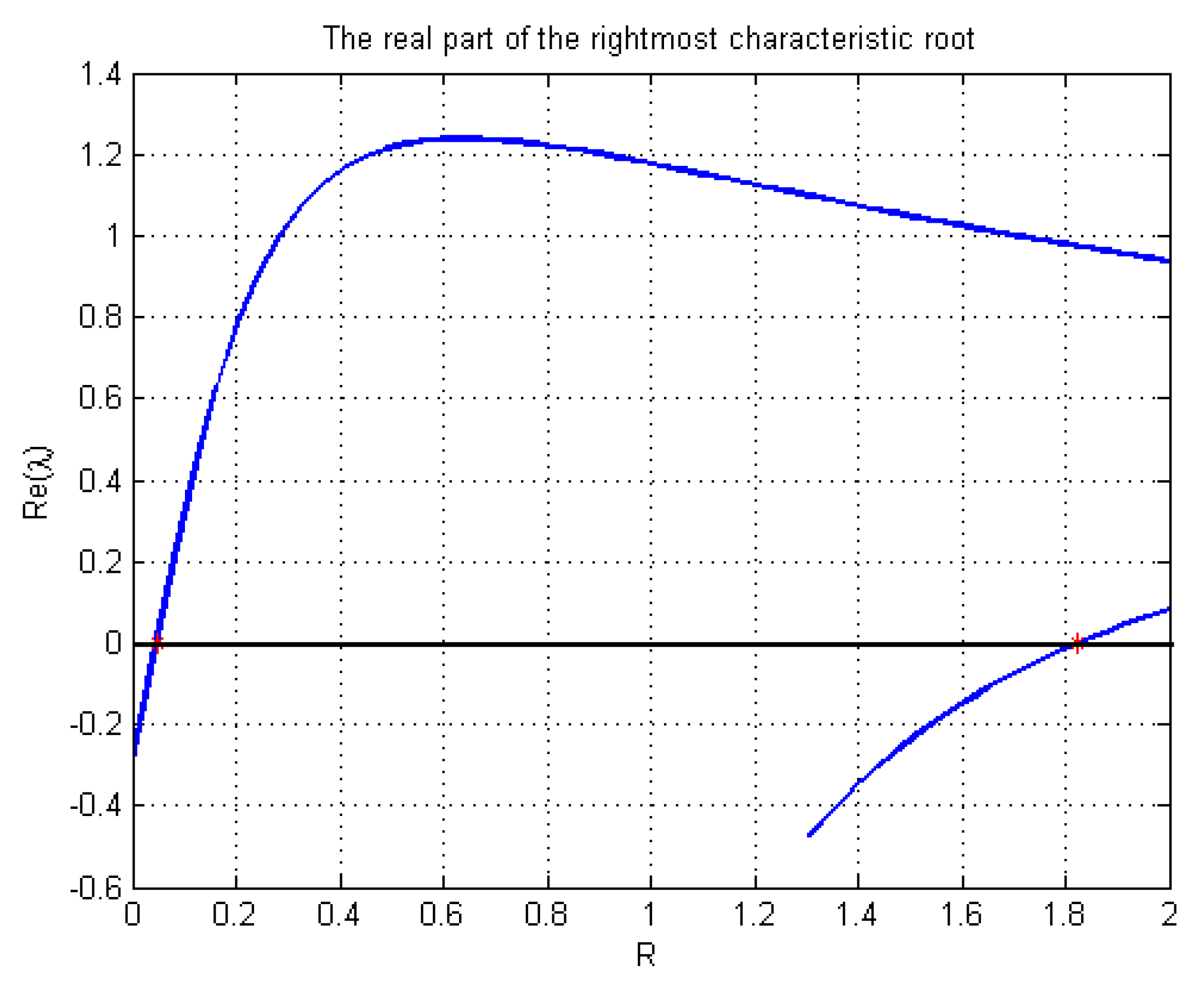
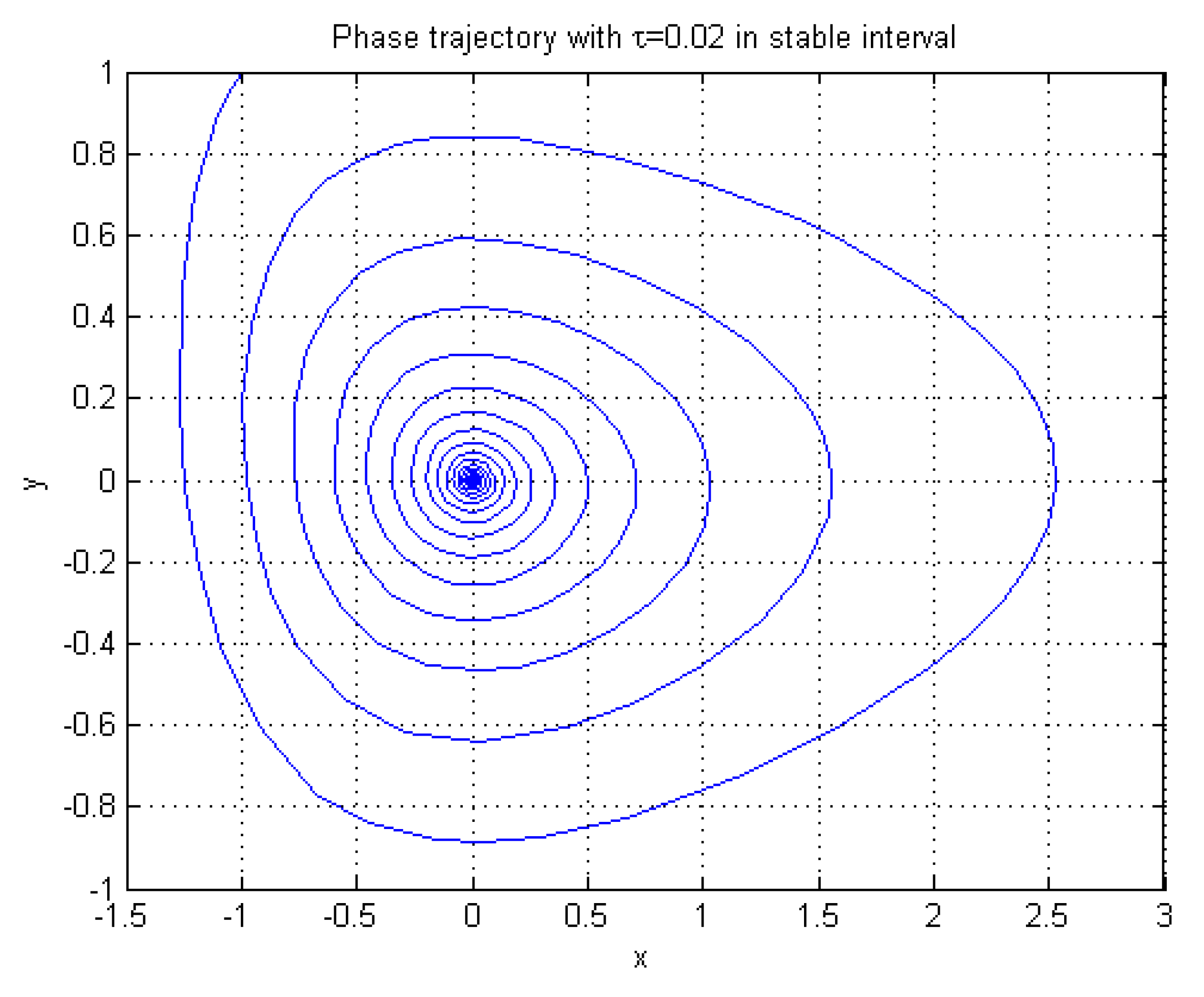
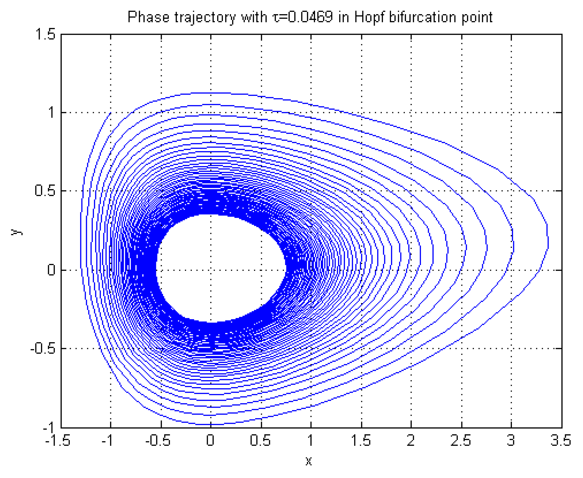
4. Numerical Examples

In this section, we will apply a typical example to show the correctness and effectiveness of our results. All of the numerical calculations are carried out by MATLAB and its powerful package of DDEBIF-TOOL 2.0. In addition, the analysis illustrates that our technique is a reliable procedure to tackle the nonlinear dynamics of a nonlinear TCP/AQM network.

Example 1.

The typical example comes from [10],

$$\begin{array}{ccc}\dot{w}\left(t\right)\hfill & =& -0.2941w\left(t\right)-0.2941w(t-R)-6.5195q(t-R)\hfill \\ \hfill & & -0.1128w\left(t\right)w(t-R)-2.5\left[w\right(t)+w(t-R\left)\right]q(t-R)-0.9587w\left(t\right)w(t-R)q(t-R)\hfill \\ \dot{q}\left(t\right)\hfill & =& 1.9173w\left(t\right)\hfill \end{array}$$

The associating characteristic equation is

$${\lambda }^2+0.2941\lambda +(0.2941\lambda +12.4998)e^{-R\lambda }$$

Proposition (1) tells us that,

$${\omega }_0=3.5355j$$

In addition, Theorem 1 leads us to the critical delay

$$R_0=0.0469$$

which is shown in Figure 1. Moreover, there is another pair of characteristic roots crossing the imaginary axis at $R_0+\frac{2\pi }{3.5355}=1.8241$. That is to say, only one delay interval exists, $[0,0.0469]$, for the TCP/AQM network. In addition, we draw stable and unstable phase trajectories in Figure 2 and Figure 3, respectively. For $R=0.05$ in Figure 3, we chose two different initial states at $(-0.1,0.1)$ and $(-1,1)$. It is easy to see that both of the two phase trajectories are convergent to the bifurcating periodic solution. In addition, this means that the equilibrium points of $(0,0)$ are unstable.

As is shown in Theorem 1, the $R_0=0.0469$ is the Hopf bifurcation point. The numerical solution can be seen in Figure 4. In addition, corresponding parameters are calculated as follows:

At first, Lemma 1 gives the adjoint vector as

$$\phi \left(\theta \right)=\left[\begin{array}{c}1\\ -0.0255j\end{array}\right]e^{j{\omega }_0\theta }\mathrm{and}{\phi }^{\ast }\left(\theta \right)=\left[\begin{array}{c}1\\ -0.0330+0.0788j\end{array}\right]e^{j{\omega }_0\theta }$$

Associating with (16) and (19), we obtain

$$g_{20}=0.0058-0.0026j,g_{11}=0.00738+0.00002jand{g}_{02}=0.0058+0.00266j$$

Subsequently, Lemma 2 $y_{20}$ and $y_{11}$ are such that

$$\begin{array}{ccc}{y}_{20}^{\left(1\right)}\left(0\right)\hfill & =& 0.00132+0.00133j\hfill \\ y_{20}^{\left(1\right)}(-1)\hfill & =& -0.001-0.0027j\hfill \\ y_{20}^{\left(2\right)}(-1)\hfill & =& -0.00002684+0.0000288j\hfill \\ y_{11}^{\left(1\right)}\left(0\right)\hfill & =& 0\hfill \\ y_{11}^{\left(1\right)}(-1)\hfill & =& 0.00159\hfill \\ y_{11}^{\left(2\right)}(-1)\hfill & =& 0.024556\hfill \end{array}$$

Thus, we have

$$g_{21}=0.0168+0.0159j$$

Therefore, the Hassard formula determines the bifurcating parameters:

$${\mu }_2=-0.0013,{\tau }_2=-0.0024and{\beta }_2=0.0168.$$

5. Conclusions

In this paper, an executable procedure is proposed for the linear stability analysis versus communication delay and calculation of Hopf bifurcation. According to the $\tau$ decomposition strategy, we provide the maximum value of delay stable boundary. Meanwhile, viewing time delay as a bifurcation parameter, we have proved that the Hopf bifurcation occurs as the delay passing this critical point. Moreover, the direction and stability of the bifurcating periodic orbits are also investigated by using the center manifold theorem, bilinear form, and projection vector. The results of the simulation study have confirmed the correctness of the theoretical results.

References

1. Misra, V.; Gong, W.-B.; Towsley, D. Fluid based Analysis of a Network of AQM Routers Supporting TCP Flows with an Application to RED. In Proceedings of the Conference on Applications, Technologies, Architectures, and Protocols for Computer Communication, Stockholm, Sweden, 28 August–1 September 2000. [Google Scholar]
2. Hollot, C.V.; Chait, Y. Nonlinear stability analysis for a class of TCP/AQM networks. In Proceedings of the 40th IEEE Conference on Decision and Control (Cat. No.01CH37228), Orlando, FL, USA, 4–7 December 2001; Volume 3, pp. 2309–2314. [Google Scholar]
3. Hollot, C.V.; Misra, V.; Towsley, D.; Gong, W.B. Analysis and design of controllers for AQM routers supporting TCP flows. IEEE Trans. Autom. Control 2002, 47, 945–959. [Google Scholar] [CrossRef] [Green Version]
4. Melchor Aguilar, D.; Niculescu, S.-I. Remarks on nonlinear stability analysis for a class of TCP/AQM networks. IFAC Proc. Vol. 2003, 36, 381–384. [Google Scholar] [CrossRef]
5. Yang, H.-Y.; Tian, Y.-P. Hopf bifurcation in REM algorithm with communication delay. Chaos Solitons Fractals 2005, 25, 1093–1105. [Google Scholar] [CrossRef]
6. Michiels, W.; Niculescu, S.-I. Stability analysis of a fluid flow models for TCP like behaviour. J. Bifurc. Chaos 2005, 15, 2277–2282. [Google Scholar] [CrossRef]
7. Guo, S.-T.; Liao, X.-F.; Li, C.-D. Stability and Hopf bifurcation analysis in a novel congestion control model with communication delay. Nonlinear Anal. Real World Appl. 2008, 9, 1292–1309. [Google Scholar] [CrossRef]
8. Ding, D.W.; Zhu, J.; Luo, X.S. Hopf bifurcation analysis in a fluid flow model of Internet congestion control algorithm. Nonlinear Anal. Real World Appl. 2009, 10, 824–839. [Google Scholar] [CrossRef]
9. Guo, S.-T.; Liao, X.-F.; Liu, Q.; Wu, H.-X. Linear stability and Hopf bifurcation analysis for exponential RED algorithm with heterogeneous delays. Nonlinear Anal. Real World Appl. 2009, 10, 2225–2245. [Google Scholar] [CrossRef]
10. Zheng, Y.G.; Wang, Z.H. Stability and Hopf bifurcation of a class of TCP/AQM networks. Nonlinear Anal. Real World Appl. 2010, 11, 1552–1559. [Google Scholar] [CrossRef]
11. Liu, F.; Wang, H.-O.; Guan, Z.-H. Hopf bifurcation control in the XCP for the Internet congestion control system. Nonlinear Anal. Real World Appl. 2012, 13, 1466–1479. [Google Scholar] [CrossRef]
12. Zhan, Z.-Q.; Zhu, J.; Li, W. Stability and bifurcation analysis in a FAST TCP model with feedback delay. Nonlinear Dyn. 2012, 70, 255–267. [Google Scholar] [CrossRef]
13. Xu, Q.; Li, F.; Sun, J.-S.; Zukerman, M. A new TCP/AQM system analysis. J. Netw. Comput. Appl. 2015, 57, 43–60. [Google Scholar] [CrossRef] [Green Version]
14. Khoshnevisan, L.; Liu, X.-Z.; Salmasi, F. Stability and Hopf bifurcation analysis of a TCP/RAQM network with ISMC procedure. Chaos Solitons Fractals 2019, 118, 255–273. [Google Scholar] [CrossRef]
15. Raina, G.; Wischik, D. Buffer sizes for large multiplexers: TCP queuing theory and stability analysis. In Proceedings of the Next, Generation Internet Networks, Rome, Italy, 18–20 April 2005. [Google Scholar]
16. Raina, G.; Manjunath, S.; Prasad, S.; Giridhar, K. Stability and performance analysis of compound TCP with REM and drop-tail queue management. IEEE/ACM Trans. Netw. 2016, 24, 1961–1974. [Google Scholar] [CrossRef]
17. Nichols, K.; Jacobson, V.; McGregor, A.; Iyengar, J. Controlled delay active queue management. RFC 2018, 8298, 1–25. [Google Scholar]
18. Lee, M.S.; Hsu, C.S. On the τ decomposition method of stability analysis for retarded dynamical systems. SIAM J. Control 1969, 7, 249–259. [Google Scholar] [CrossRef]
19. Walton, K.; Marshall, J.E. Direct method for TDS stability analysis. IEEE Proc. D Control Theory Appl. 1987, 134, 101–107. [Google Scholar] [CrossRef]
20. Cooke, K.; Driessche, P. On zeros of some transcendental equations. Funkc. Ekvacioj 1986, 29, 77–90. [Google Scholar]
21. Hassard, B.D.; Kazarinoff, N.D.; Wan, Y.H. Theory and Applications of Hopf Bifurcation; Cambridge University Press: Cambridge, UK, 1981. [Google Scholar]
Figure 1. The rightmost root loci versus delay R.
Symmetry 14 00463 g001
Figure 2. The stable phase trajectory with delay in stable interval.
Symmetry 14 00463 g002
Figure 3. The two phase trajectories with delay in unstable interval.
Symmetry 14 00463 g003
Figure 4. The bifurcating phase trajectory with delay in Hopf bifurcation point.
Symmetry 14 00463 g004
Publisher’s Note: MDPI stays neutral with regard to jurisdictional claims in published maps and institutional affiliations.