
Searching Mass-Balance Analysis to Find the Composition of Martian Blueberries


Two Planet Life, West Bloomfield, MI 48324, USA
Minerals 2022, 12(6), 777; https://doi.org/10.3390/min12060777
Submission received: 23 March 2022
/
Revised: 13 June 2022
/
Accepted: 17 June 2022
/
Published: 18 June 2022
(This article belongs to the Topic Study of Minerals by Molecular Spectroscopy)
Abstract
:Between 2004 and 2018, NASA’s rover Opportunity found huge numbers of small, hematite-rich spherules (commonly called blueberries) on the Meridiani Planum of Mars. The standard oxide composition distributions of blueberries have remained poorly constrained, with previous published analyses leaving hematite content somewhere in the broad range of 24–100 wt%. A searching mass-balance analysis is introduced and applied to constrain possible standard oxide composition distributions of blueberries consistent with the non-detection of silicates in blueberries by Opportunity’s instruments. This analysis found three groups of complete solution sets among the mass-balance ions consistent with the non-detection of silicates; although, a simple extension of the analysis indicates that one larger space of solutions incorporates all three groups of solutions. Enforcing consistency with the non-detection of silicates in blueberries constrains the hematite content in most of blueberry samples to between 79.5 and 99.85 wt%. A feature of the largest group of complete solution sets is that five oxides/elements, MgO, P2O5, Na2O, SO3, and Cl, collectively have a summed weight percentage that averages close to 6 wt%, while the weight percentage of nickel is close to 0.3 wt% in all solutions. Searches over multidimensional spaces of filtering composition distributions of basaltic and dusty soils were a methodological advance.
1. Introduction
NASA chose to land its Mars Exploration Rover (MER) Opportunity on the Meridiani Planum [1,2]. This is a plain with an area larger than Lake Superior that straddles the equator of Mars [3]. In the late 1990s and early 2000s, a thermal emission spectrometer (TES) orbiting above Mars (in the Mars Global Surveyor) found signals of surface crystalline, grey hematite (Fe2O3) across the plain [1,2]. Edgett [3] and this TES hematite data provided evidence for abundant flowing water in the plain’s far past [4,5], because hematite only forms in the presence of water. NASA considered the plain an excellent place to search for signs of life [2].
Opportunity made a bouncing landing into Eagle Crater on the plain in January 2004 [6]. The very first image taken by the scientific PanCam had poor exposure [7], but it showed an expanse of soil spread from the bottom of the 22 m diameter crater to its rim and, near the limit of the camera’s resolution, the image showed the soil covered with thousands of small spherules. In the following sols (Martian days), Opportunity’s team found that the small spherules are rich in grey hematite [7,8,9,10,11], and, when seen against rusty-red soils, that they look blue. The team quickly called them blueberries.
Opportunity’s PanCam directly imaged huge numbers of blueberries during the rover’s years-long traverse from Eagle Crater to Endeavour Crater [12,13,14,15,16]. It was soon realized that loose blueberries on top of the soil were probably responsible for the regional-scale (>150,000 km2) surface hematite detection made earlier by the orbiting TES [16].
Given the prominence and ubiquity of blueberries on the Meridiani Planum, the composition of blueberries was obviously a matter of interest, and Opportunity’s team of scientists collected a large amount of relevant data with the rover’s instruments (more below). Seven papers published in a single issue of Science in late 2004, each addressed the issue of the composition of blueberries to a larger or lesser extent using data from all the instruments on the rover [8,9,10,11,15,16,17]. However, the lead and summarizing paper, i.e., [16], of this issue of Science that was dedicated to presenting Opportunity’s first 7–9 months of data collection, could only state with confidence “that their [blueberries] composition is dominated by hematite”. Explaining difficulties in determining blueberry composition, this lead paper stated: “Because the spherules are much smaller than the fields of view of the APXS and Mössbauer instruments, it is not possible to isolate individual spherules for detailed compositional analysis by these instruments” [16]. To try to make progress with blueberry composition, in 2005, a team of Opportunity’s scientists led by Richard Morris made a detailed study of analogs of blueberries found on the slopes of the volcano Mauna Kea on the large island of Hawaii [18]. These analogs had hematite weight percentages between 90% and 91% [18]. The only previously published, peer-reviewed paper to state a quantitative range for hematite content in actual blueberries on the Meridiani Planum appeared in 2006 [19]: the paper only constrained the range to 24–100 wt% [19]. Various NASA conference abstracts in 2005, 2006, and 2007 made tentative statements about blueberry composition, more below. Following the results of very high hematite content in the Hawaiian analogs [18], the 2006 paper showed that a mass balance analysis of the available data was consistent with a blueberry composition of 99.7 wt% hematite and 0.3 wt% nickel [19]. This paper also implied (correctly) that mass balance analysis of the APXS and Mössbauer data, without extra constraints, was insufficient to constrain the hematite content in blueberries tighter than the 24–100 wt% range it published. However, in 2009, the Opportunity team published another major paper on blueberries that included an important result for the present paper: Opportunity’s miniature thermal emission spectrometer (Mini-TES) could not detect any silicates in the blueberries [12]. This non-detection of silicates is here used as an extra constraint for mass-balance analyses of the composition of blueberries. This extra constraint effectively narrows the possible hematite weight percentages of blueberries to high values, given the data from all of Opportunity’s instruments.
This paper is a data analysis and methods paper. The data analyzed comes from public domain databases; particularly important here is Opportunity’s alpha-particle x-ray spectrometer (APXS) oxide abundance (weight percentage) database [20].
In Section 2 Materials and Methods this paper will:
- 1.
- Review the instruments that measured the composition of blueberries, in particular, the mixed signals the instruments actually captured;
- 2.
- Review papers that added constraints for this analysis and previous abstracts and the paper that applied mass-balance analysis to the composition of blueberries;
- 3.
- Describe the choice of input APXS data used here, i.e., from among the entire APXS database;
- 4.
- Describe the demixing problem, i.e., inferring blueberry compositions from mixed signals from mixed materials. Introduce spaces for filtering distributions of basaltic soil and dusty soil compositions;
- 5.
- Describe the searching mass-balance analysis demixing procedure.
This is followed by the Results, Discussions, and Conclusions sections.
The use of the spaces of filtering distributions and searching mass-balance analysis is novel. These are both described in detail.
2. Materials and Methods
2.1. Review: Opportunity’s Instruments and Mixed Signals
Several of the scientific instruments on the rover Opportunity collected data useful for determining the composition of blueberries. The most focused for composition determinations were a Mössbauer spectrometer [21] and an APXS [22]. However, Opportunity’s Mini-TES [23], Microscopic Imager (MI) [24], PanCam [7], and even its rock abrasion tool [25] all contributed data relevant to the composition of blueberries.
The Mössbauer spectrometer collected data on the abundances of minerals containing iron, while the APXS instrument collected data on the abundances of 16 elements commonly found in rocks, soils, and dust, although, APXS abundances are reported as standard oxide abundances rather than as elemental abundances [22]. Several important papers report APXS and Mössbauer data [8,11,16,19,26]. The early “berry bowl” Mössbauer spectrometer experiment showed that hematite dominates the iron-containing minerals in blueberries [8].
Opportunity’s MI made many images of interior sections of blueberries, both freshly cut by the rock abrasion tool and in blueberry fragments. These sections consistently showed that blueberries have homogeneous interiors without features resolvable at the MI’s 30–32 bits per pixel resolution [16]. This homogeneity makes it possible to extrapolate APXS and Mössbauer surface results to whole blueberries.
The Mössbauer spectrometer and the APXS were used with similar surface data collection techniques; that is, each instrument was positioned at a fixed distance from the surface of target materials to be measured using a robot arm and surface contact plates, then the instruments emitted radiation onto the targets, and simultaneously sensed, measured, and recorded back-radiation.
The input data to a blueberry composition analysis, from either the Mössbauer spectrometer or the APXS, are mixed-signal data from multiple materials. There are two points to make about how and why this is so. The first is that the fields of view of both instruments were large relative to the view area of a single blueberry, even a large one [16,21,22]. Therefore, the composition signals from blueberries were mixed with those from laterally adjacent materials [16]. The second is that layers of dust cover all surface materials on Mars, and the thicknesses of these layers are not negligible relative to the sampling depth of the Mössbauer spectrometer and the APXS [19,27]. Thus, as Opportunity had no means to clean the dust off the collections of loose blueberries, the composition signals of blueberries were also mixed with those of dust [19,27,28,29]. Further, although the sampling depth of the Mössbauer spectrometer was shallow (0.2–3 mm) [21], that of the APXS was shallower (0.02 mm) [22]; Morris et al. (2006) emphasized that the two instruments sensed significantly different material mixtures, even when placed over the same sample targets [19].
2.2. Review: Blueberry Composition & Early Mass-Balance Analysis
A necessary part of any mass-balance analysis are computations using constraint equations, constraint bounds, and constraint sums. However, such mathematical constraints are never enough with mixed-material signals. Additional constraints are needed. The present analysis uses experimental data to add constraints.
Opportunity’s PanCam and Mini-TES instrument made measurements that indicate that blueberries have high levels of crystalline hematite [9,10,12]. These results are not specific enough to draw highly resolved hematite fractions in blueberries. However, any APXS data demixing should find high levels of iron oxide content, and any Mössbauer data demixing should find high levels of hematite.
Opportunity’s Mini-TES instrument made even more critical measurements for strongly restricting the possible compositions of blueberries; that is, this Mini-TES could not detect silicate minerals above its detection threshold [12]. This null result imposes an upper bound on the size of the SiO2 fraction in APXS blueberry compositions.
The reported mass-balance results are similar to features of basalt and spherule analog composition, in Mars meteorites landed on Earth [30], in native Earth basalts [31,32], and Mars analogs on Hawaii [18]. These features were used indirectly in the searching mass-balance analysis to infer the composition of blueberries through the influence of Morris et al. (2006), [19], on the searching procedure, an elaboration is given in the sub-section on the searching mass-balance procedure.
In 2005, Jolliff was the first to perform mass-balance analysis on material mixtures to determine the composition of blueberries [27]. Morris et al. followed in 2006 [19], and Jolliff et al. made another short analysis in 2007 [29].
Morris et al. only considered cases in which the mixed-materials containing blueberries included just three component materials: blueberry material, basaltic soil, and dust [19]. This is sensible, as (A) Opportunity’s sample targeting focused on these cases, and (B) considering blueberry mixtures containing four or more component materials, such as blueberries, basaltic soil, dust, and sediment rock, complicates the analysis. In Jolliff’s first, short 2005 discussion of blueberry demixing, he considered mass-balance analysis on a three-component mixture of blueberry material, basaltic soil, and rock, and he also mentioned this did not account for the effect of dust. The principal mass-balance equation for analyzing mixtures of blueberry material, basaltic soil, and dust is:
In the above equation and are weight percentages for the mixture material , the blueberry material either whole blueberries and/or blueberry fragments, the basaltic soil , and the dust (D); while and are mixing fractions (which sum to 1) for the blueberry material, the basaltic soil, and the dust. Further, in Equation (1), the subscript index that appears in the weight percentages (such as ) is an index indicating either a chemical species (for example, SiO2) in APXS data, or an iron-containing mineral (for example, olivine) in Mössbauer spectrometer data. Equation (1) is, in fact, a set of equations, one each for each possible value of the index, and these equations need to be solved simultaneously. For Opportunity’s APXS data the index ranges over 16 species of oxides and elements.
In 2006, Morris et al. tested an extreme oxide composition case for blueberries with 99.7 wt% FeO/Fe2O3, 0.3 wt% Ni, and 0 wt% for all the other 14 oxide/elements [19]. That is, this test assumed a specific blueberry composition, and it guessed mixing fractions, used an average mixed-material composition, and plugged all these values into the set of 16 equations of Equation (1) to compute a composition of mixed basaltic and dusty soils [19]. They then compared this computed mixed soil distribution to an average mixture of basaltic and dusty soils. These two mixed soil distributions looked very similar to the eye. Morris et al. had succeeded in showing that mass-balance analysis of blueberry/basaltic soil/dusty soil mixtures allowed blueberry compositions with close to 100% hematite content. However, in their conclusions, the iron oxide content of blueberries was only weakly restricted to a broad range: 24–100 wt%. Without additional experimental constraints, this broad range is reasonable: mass-balance analysis can be applied to blueberry/basaltic soil/dusty soil mixtures using other mixing fractions and small changes to the compositions of filtering distributions to come up with blueberry compositions with low iron oxide content.
Jolliff et al.’s 2007 conference abstract on blueberry composition applied Equation (1) using two pairs of sets (of assumed) mixing fractions [29]. They computed blueberry weight percentages in the four cases by solving Equation (1) after inputting their own values on the mixing fractions and averaged composition values for the mixed-materials, basaltic soil, and dusty soil. The values of the mixing fractions had been chosen so that small changes to the non-zero mixing fractions produced blueberry compositions that flipped from being allowable to dis-allowable, that is, their computations produced some blueberry weight percentages that were negative—negative weight percentages are not physically possible. They then suggested these results imposed upper limits of around 60 wt% on the Fe2O3 percentages in blueberries [29]. However, their upper limit was far below the allowable 99.7% Fe2O3 weight percentage Morris et al. demonstrated. Further, at their upper limit on iron oxide content, their computed SiO2 weight percentages were close to 20 wt% [29]; these SiO2 weight percentages are not reconcilable with the Mini-TES results on the silicate content of blueberries [10,12].
2.3. Choice of APXS Data
The APXS data analyzed in this paper comes from Opportunity’s oxide abundance database stored in the file apxs_oxides_mer1.Opportunity.csv [20].
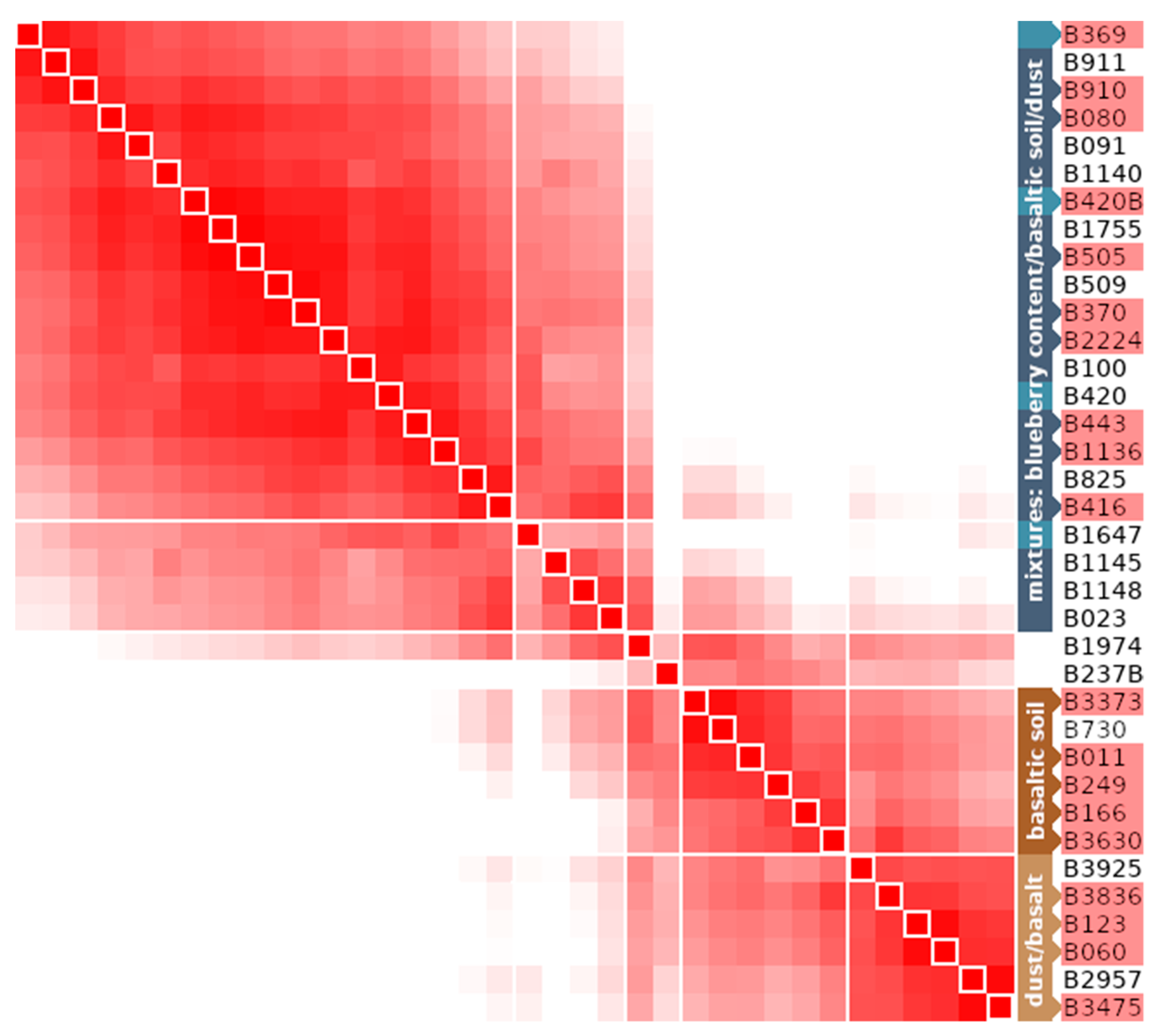
Each record in the database file is a composition distribution measured from a sampling target by the APXS instrument. Only some of the distributions in the APXS database file are used in demixing to determine the compositions of blueberries. The choices of which distributions to input to demixing computations were made using: (I) the documentation for the database file, (II) a distribution clustering procedure (more below), (III) visual checks of Opportunity’s MI images taken to document the sampling targets from which the APXS took distribution measurements. The list of identifiers of APXS distributions used in demixing is given in Table 1. The relevant images taken by Opportunity’s MI are in NASA’s Opportunity Microscopic Imager raw image archive [33]. Figure S1 in the Supplementary Material reproduces the rover’s MI images from the actual mixed-material sampling target locations with distributions chosen for demixing (listed in Table 1), as well as example images of basaltic soil and sandy soil distributions (also listed in Table 1). The distribution clustering to identify distributions was achieved by (A) computing a matrix of similarity distances between all pairs of composition distributions for the database’s 36 composition distributions for undisturbed soils, followed by (B) matrix blocking. The blocked matrix is shown in Figure 1, with the pairwise similarity distance values converted to a monochrome (red-to-white) scale. The pairwise distances computed for this matrix were Jensen–Shannon distances. Jensen–Shannon distances are used to compare distributions; they are the square roots of other distribution similarity measures, called symmetric relative entropies or Jensen–Shannon divergences; a readable reference is the Wikipedia page for Jensen–Shannon divergences. An alternative pairwise similarity distance metric, the norm of the scalar (dot) product, produces the same blocked matrix basis order as Jensen–Shannon distances. Additional details on how the distributions were chosen are given in Appendix A. The shortened database IDs will be used here to identify the distributions.
The weight percentages of the chosen mixed material distributions are reproduced (from the APXS database [20]) in Table 2 in the order given in the largest matrix block in Figure 1. This order makes visible rising and falling weight percentage trends across the table rows, for some of the abundant oxides such as CaO, Al2O3, SiO2, and FeO, and also for some of the other oxides/elements that will be important for the demixing, including TiO2, K2O, and Ni, as well as the lack of rising/falling trends for some oxide/elements including MgO, P2O5, Na2O, SO3, and Cl, again these relatively constant weight percentages fractions will be important in demixing. Computed Pearson correlation coefficients (not shown) comparing the weight percentages in Table 2 for CaO, Al2O3, SiO2, TiO2, K2O, FeO, and Ni show strong positive correlations between the weight percentages of all of CaO, Al2O3, SiO2, TiO2, and K2O, strong anti-correlations between the weight percentages of all of these oxides and those of both FeO and Ni, and a strong positive correlation between the weight percentages of FeO and Ni.
Five of the basaltic soil distributions and four of the dusty top-layer distributions were chosen (see Figure 1 and Table 1) as filtering distributions in the demixing computations. The weight percentages for these filtering distributions are reproduced in Table 3 from the APXS oxide abundance database, with the ordering of distributions following that of the second-largest matrix block matrix Figure 1.
2.4. The Demixing Problem & the Spaces of Basaltic Soil and Dusty Soil Distributions
Mass-balance analysis of mixed-material signals to find the composition of one material (e.g., blueberries) in the mixture is a filtering procedure to subtract (filter) the potential signals from the mixture’s other materials (e.g., basaltic soil and dusty soil) from the mixed signals (e.g., the data in Table 2) to uncover the composition signal from the material of interest (blueberries). Using averaged basaltic and dusty soil distributions as filters on the mixed signals failed to find blueberry compositions consistent with the non-detection of silicate minerals by the Mini-TES instrument. There is variety in the ten mixed-material sampling targets shown in Figure S1 and between the distributions given in Table 2 and Table 3. Moreover, there is no accurate and precise knowledge of the composition of the basaltic and dusty soils at each sampling site, although, there is information (in Table 3) on the compositions of basaltic and dusty soils at various other sampling locations. Given this, it makes sense to search thoroughly with different, acceptable pairs of filtering distributions (where one is a possible basaltic soil distribution, and the other is a possible dusty soil distribution) and, with each different filtering pair, to subtract signals to find an example blueberry composition. Furthermore, to then repeat this to find many blueberry composition examples that are consistent with the non-detection of silicate minerals in blueberries. The above is an outline of the searching mass-balance analysis done to produce the results reported here. The main search is over pairs of distributions. Section 2.5 gives more detail. The next thing to do is describe the spaces of composition distributions of basaltic and dusty soils.
Opportunity’s APXS measured each basaltic soil and dusty soil distribution in Table 3 at specific sampling locations along the rover’s traverse across the plain from Eagle Crater to Endeavour Crater. The physical distances between some pairs of these sampling locations were over 20 km, for example, the sampling locations for the two basaltic distributions B3373 and B011. The five basaltic soil distributions given in Table 3, i.e., B3373, B011, B249, B166, and B3630, should collectively represent practical guides as to how much variety in basaltic soil distributions could be measured across the parts of the plain traversed by Opportunity. Similarly, the four dusty soil distributions, i.e., B3836, B123, B060, and B3475, should collectively represent practical guides to the variety of dusty soil distributions. This paper will use these two collections to define spaces of basaltic soil and dusty soil distributions.
The space of dusty soil distributions and the space of basaltic soil distributions are both defined as a central core space plus an extension layer around the core. The central core space of dusty soil distributions is, for our practical purposes, all those distributions that can be made “in-between” the four experimentally measured dusty soil distributions, i.e., B3836, B123, B060, and B3475, as linear combinations of these four experimental distributions (with non-negative mixing fractions that sum to 1). Similarly, the central core space of basaltic soil distributions is all those distributions that can be made “in-between” the five experimentally measured basaltic soil distributions, i.e., B3373, B011, B249, B166, and B3630.
A helpful analogy for these core spaces is a room. The “room” for the dust core space is a tetrahedron with the four experimental distributions (B3836, B123, B060, and B3475) forming the room’s “corners,” that is, the tetrahedron’s vertices. Any “in-between” distribution is a point inside the room. The distances between any interior point to one of the room’s corners tend to be shorter than those from one corner to another. With Jensen–Shannon distance measurement, this is also a feature of the interior dusty soil distributions and the “corner” experimental distributions (B3836, B123, B060, and B3475). Similar comments hold for the basaltic soil core space defined by the five experimental distributions, B3373, B011, B249, B166, and B3630, except now the “room’s” shape is a hexahedron with five vertices or corners. Note the two core “rooms” contain the average basaltic soil and dusty soil distributions. These average distributions are at the rooms’ centers. The practical point about having an extension layer around the cores is that the APXS distribution data is incomplete. Opportunity’s APXS could have sampled other basaltic soil or dusty soil targets and made distribution measurements that fall outside the core spaces. In fact, Opportunity’s APXS made measurements that did exactly this: the dusty soil distribution B3925, shown in the blocked distance matrix in Figure 1, is outside the core space for dusty soil distributions. By definition, a distribution is considered to be inside the extension layer of the basaltic soil space when (a) it is not in the basaltic soil core space, and (b) the distance between this distribution and any one of the core space distributions is less than or equal to a maximum allowed layer thickness, denoted LT, where this distance is measured either as the Jensen–Shannon distance or as the norm of the scalar product between the two distributions. The definition for the dusty soil case is similar; just replace “basaltic soil” with “dusty soil” in the last sentence. So, now there is a question of what is a suitable value for LT? It is good to use Opportunity’s actual data, so, for now, LT is set equal to the Jensen–Shannon distance between the B3925 distribution (outside the dusty soil core) and the measured core dusty soil B3836 distribution. Note, B3925 is closer to B3836 than the other measured dusty soil distributions, B123, B060, and B3475. However, further analysis of the data might provide reasons to change this initial value for LT. With this layer thickness value set LT = 0.065, and the B3925 distribution is on the boundary of the allowed space of dusty soil distributions.
2.5. Searching Mass-Balance Demixing Procedure
Ten searching investigations were carried out. Each of these ten investigations was for one of the ten mixed-material distributions listed in Table 2. Each single investigation consisted of 1,336,608 (1,336,608 = 13 × 126 × 816) attempts to find a complete solution set to the collection of 16 of mass-balance equations (for all of the 16 oxide indices) given by Equation (1). A complete solution set consists of (A) a set of three mixing fractions (i.e., and in Equation (1)), and (B) three demixed composition distributions (one each for blueberries, basaltic soil, and dusty soil) for the 16 APXS oxide/elements. To be a complete solution set, for each of the 16 oxide/element cases indexed with k, the three weight percentages ( and in Equation (1)) from the three composition distributions and their corresponding mixing fractions ( and ) are plugged into the right-hand-side of Equation (1) and precisely compute a value of the weight percentage (left-hand-side of Equation (1)) and this computed has to be equal the actual from the mixed-material distribution under investigation. Emphasizing, equality between the computed right-hand-side and the actual must hold for all k for any complete solution set to be valid. The goal of these searching investigations is to find many complete solution sets where the weight percentage value of SiO2 in the blueberry distribution () is low and consistent with the non-detection of silicates in blueberries by Opportunity’s Mini-TES.
For each of the ten investigations, the following was done:
- For each of 13 sets of target constraints (more below), a large number (102,816) of input pairs of basaltic soil and dusty soil distributions were each individually sent to a procedure that varied the basaltic soil distribution and computed a set of the mixing fractions and a full set of blueberry weight percentages (collectively a blueberry composition distribution);
- Each individual variation and computation could fail or succeed at discovering an acceptable complete solution set that solved Equation (1) (up to 64-bit computer accuracy) for the individual mixed-material distribution under demixing investigation. If any one of the 1,336,608 tests/attempts succeeded, then all information for that test/attempt was made into a complete solution set record and stored in a database file of successful example records of complete solutions sets.
The database file, documentation, and a Perl script to help interact with the database are publicly available at the Zenodo repository [34].
The 102,816 pairs of initial basaltic soil and dusty soil distributions were all combinations of a list of 126 basaltic soil distributions and another list of 816 dusty soil distributions (102,816 = 126 × 816). The 126 basaltic soil distributions were part of the core space of basaltic soil distributions. Five of these were the “corner” measured distributions (in Table 3), the remaining 121 were interior distributions in the basaltic core space. Collectively (by construction), these 126 basaltic soil distributions evenly sampled the basaltic soil core space. Similar construction methods made the 816 dusty soil distributions in the core of dusty soil space but with a denser sampling. The numbers 126 and 816 arise due to combinatorics; further construction details are in Appendix B.
The use of 13 sets of target constraints mentioned in the above outline was motivated by Morris et al. [19]. That paper used the authors’ experience with geology, Hawaiian blueberry analogs [18], and blueberries to suggest that weight percentages of many APXS oxides were likely to be extremely small or 0%.
In an effort to both use the idea of constraining some of the oxide/element weight percentages to 0% (with is computationally helpful) and also to be deliberate about how many and which oxide/element weight percentages to constrain to 0%, plots of the various oxide weight percentages (found in Table 2) were made against the weight percentages of FeO (also in Table 2). The collection of these plots (not shown) suggested the following ordering of oxides most likely to have 0 wt% in blueberries (from most likely to quite possible): CaO and TiO2, K2O, MnO, Cr2O3, Al2O3, and SiO2. In addition, the weight percentages for bromine (Br) are always so low and had other features (see discussion) that the computations could easily find some basaltic soil/dusty soil pairs that could accommodate setting the Br weight percentage to 0% (even with Br’s mildly positive correlation with FeO). Although Zn also has very low weight percentages (see Table 2 and Table 3), these are generally higher weight percentages than those of Br, and the Zn data does not have the confusing features that Br data has, further Zn is also moderately positively correlated to FeO, so it is hard to accommodate a 0 wt% for Zn using fine variations in soil compositions. Although MgO is noticeably anti-correlated to both FeO and Ni in mixed material distributions, this anti-correlation is not so strong as those between FeO and CaO, TiO2, K2O, Al2O3, and SiO2, while the weight percentages for MgO in mixed materials are high. This combination of abundance and only moderately strong anti-correlation to FeO makes it more likely that blueberries contain some MgO than blueberries containing any of CaO, TiO2, K2O, Al2O3, and SiO2. In addition, the weight percentages for all of P2O5, Na2O, SO3, and Cl in mixed materials are only weakly correlated or anti-correlated with those for FeO and Ni, and the weight percentages of these species in mixed material are much larger than those of Br, Zn, and Ni. So, for all of P2O5, Na2O, SO3, and Cl, there are significant uncertainties as to whether or not these species appear in blueberries. Given the above discussion, the 13 sets of constraints used in the searching demixing program were sequentially constructed to be more and more restrictive. The first set constrained the weight percentages of only CaO and TiO2 to 0 wt%. Continuing with addition by one, the seventh set of constraints fixed the weight percentages to 0 wt% for these eight oxides/elements: CaO, TiO2, K2O, MnO, Cr2O3, Al2O3, SiO2, and Br. The most restrictive (thirteenth) set only left FeO and Ni free and enforced 0 wt% on the other fourteen oxide/elements.
For each input mixed material distribution, the initial program has three levels of searching. The two obvious ones are the surveys over (I) the input pairs of soil distributions and (II) the list of 13 (0 wt%) constraint sets. The third level of search is through variations to the input basaltic soil distribution. These variations are computed in 12 × 102,816 out of the 13 × 102,816 tests run for each mixed material investigation. In the least restrictive constraint set, with just two 0 wt% constraints (i.e., those for CaO and TiO2), these two constraints can be satisfied by adjusting the two free parameters of the three mixing fractions. That is, in this least restrictive case, this adjustment fixes the values of the mixing fractions. In the other 12 cases, the list of constraints cannot be satisfied solely by adjusting the values of the mixing fractions. In these cases, the basaltic soil distributions are varied (in addition to varying the mixing fractions) to enforce the longer list of 0 wt% constraints. A least-squares optimization procedure (to satisfy the given set of 0 wt% constraints) controls the variations made to the basaltic soil distributions and the mixing fractions. Because in each of the 12 × 102,816 tests the input basaltic soil distributions are varied, the number of these input basaltic soil distributions (i.e., 126) should be smaller than the number of unvaried dusty soil distributions (i.e., 816). Note the database of complete solution sets contains some solutions that might have varied basaltic soil distribution that fall outside the allowed space of basaltic soil distributions [34]. Database users can filter out such distributions by rejecting any that have Jensen–Shannon distances (included in all records of complete solution sets) above the layer thickness cut-off of 0.065.
Limitations with this searching procedure are discussed later.
3. Results
The searches found three groups of complete solution sets of Equation (1) with blueberry SiO2 weight percentages low enough that the Mini-TES may not have detected any silicate minerals.
Table 4 presents three examples of complete solution sets from the largest group. These solution sets are called ES1 (Example Solution 1), ES2, and ES3. All three sets are complete solutions sets for the B370 mixed-material distribution, one of the ten distributions listed in Table 2. Sets ES1, ES2, and ES3 are also experimentally relevant complete solution sets (ERCSS): an ERCSS is a complete solution set consistent with the non-detection of SiO2 by Opportunity’s Mini-TES. These three examples were chosen from many thousands of similar complete solution sets (more below). These three examples are not better than many other complete solution sets. They are just examples of complete solution sets that are also ERCSSs. Although ES3 is a borderline case, as its 8 wt% for SiO2 may be too high for a non-detection of silicate minerals by Opportunity’s Mini-TES instrument. The Mini-TES mineral abundance measurements were accurate to within 5–10 wt% [5]. The example solution sets ES2 and ES3 were computed with six oxides (CaO, TiO2, K2O, MnO, Cr2O5, and Al2O3) constrained to 0 wt%. The ES1 was computed with those six oxides plus SiO2 constrained to 0 wt%. The normalized version of distribution B370, with a total weight percent sum of exactly 100%, is in the left column of Table 4 to six decimal place accuracy. Similarly, the mixing fractions and the weight percentages of the three complete solution sets are all given to four decimal place precision; the full records store at 15 decimal place precision or more [34]. This precision does not imply a high level of certainty in our knowledge of blueberries, basaltic soil, and dusty soil compositions. Instead, each complete solution set is just one of many solutions that all solve the mass-balance Equation (1) with equally high precision. Collectively, the multitude of complete solution sets generate ranges of possible compositions for blueberries, basaltic soils, and dusty soils (and the mixing fractions of these). The reason such high precision is used in the searches is to find actual solutions to the mass-balance equations Equation (1)—the calculations to find these solutions are sensitive to small changes.
Table 5 and Table 6 give some Jensen–Shannon distances. These provide some information on the distances between distributions in the space of basaltic soils, and on the sizes of variations between input basaltic soils (to the surveying search) and the varied basaltic soils that provide (exact) complete solution sets.
Table 5 gives a matrix of Jensen–Shannon distances between the five experimentally measured basaltic soil distributions in Table 3 and the three Input Basaltic Soil distributions (IBS_ES1, IBS_ES2, and IBS_ES3) to the computations that produced the example solutions listed in Table 4. For solution ES1, the input distribution IBS_ES1 is one the measured distributions (B3373), so IBS_ES1 is not one of the “interior” distributions, but a “corner” distribution of the core. For solutions ES2 and ES3, the input distributions IBS_ES2 and IBS_ES3 are both “interior” distributions.
The distances between the two “interior” distributions (IBS_ES2 & IBS_ES3) and the corner (measured) distributions are mostly smaller than the distances between one measured distribution and another: Table 5 gives examples of distances consistent with the analogy between a room and the core space of basaltic soil distributions.
Table 6 gives Jensen–Shannon distances between the input basaltic soil distributions and the final Varied Basaltic Soil distributions (VBS_ES1, VBS_ES2, and VBS_ES3) listed in the basaltic soil columns of Table 4. These distances are all smaller than the layer thickness, LT = 0.065, defined in Section 4. The database of complete solution sets contains a small fraction of solutions where the Jensen–Shannon distance of variation is above 0.065, unlike those in Table 6. There is a possibility that such solutions use distributions for basaltic soils that may fall outside the allowed space of basaltic soil distributions. Such solutions were not used for the statistics reported here.
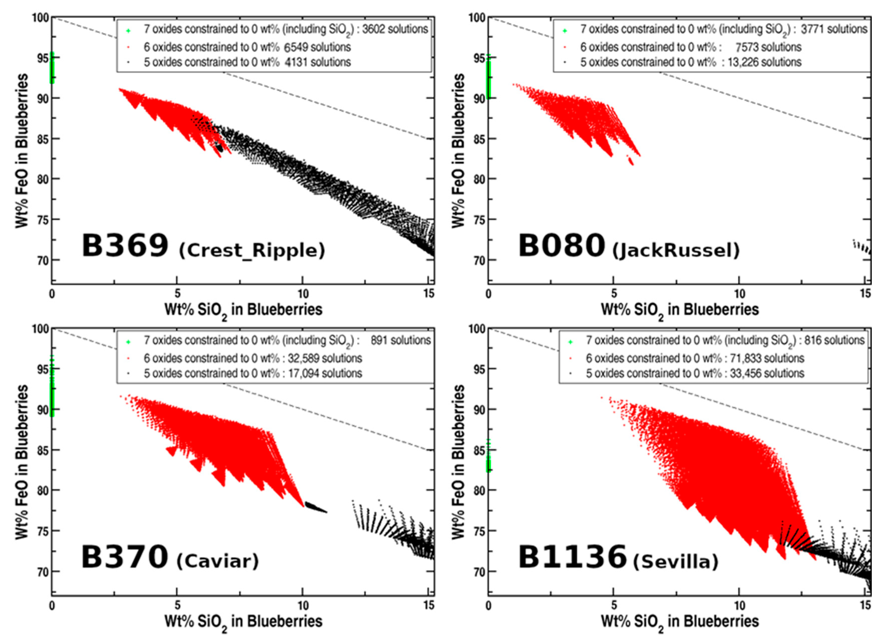
The four scatter plots in Figure 2 present partial information about 189,531 complete solution sets where either five, six, or seven of the APXS oxides were constrained to 0 wt%. These scatter plots use partial information from investigations of four mixed-material distributions: B369, B080, B370, and B1136. The scatter plots give FeO versus SiO2 blueberry weight percentages. The legend boxes give the number of times a complete solution set was successfully computed among 102,816 computational tests run for each constraint set for each mixed-material distribution investigated. Complete solutions sets where the previous seven oxides plus Br were constrained to 0 wt% could be used to add more points to the Figure 2 scatter plots. However, these points coincided with the points from the seven oxide constraint tests. Scatter plots for the other six mixed-material distributions (i.e., B910, B420B, B505, B2214, B443, and B416) were similar to those shown in Figure 2.
The scatter plots in Figure 2 only reach SiO2 weight percentages of 15 wt%. However, other complete set solutions had higher SiO2 weight percentages and lower FeO weight percentages. These solution sets, with higher blueberry SiO2 content, were computed using constraint sets where either two, three, four, or (sometimes) five of the oxides were constrained to 0 wt%. The scatter plot continuations to higher SiO2 weight percentages produce straight extended bands. The FeO and SiO2 weight percentages are strongly anti-correlated with Pearson coefficients between −0.9 and −1.0. The complete solutions sets with higher (above 15 wt%) SiO2 content in blueberries were not consistent with the Mini-TES instrument’s non-detection of silicate minerals in blueberries.
An important point to realize about the scatter plots in Figure 2 is that they are somewhat misleading. They are misleading in that they are not showing +’s at all the locations where they could be placed. More complete scatter plots would be thick linear bands with the green, red, and black “blobs” joined together. The gaps seen between the “blobs” in Figure 2 are artifacts of the details of the initial searching mass-balance analysis program. This point is returned to in the discussion.
Table 7 gives the number of times a complete solution set was successfully computed among 102,816 computational tests run for different constraint set cases for all the mixed-material distributions investigated. Some constraint set cases do not appear in Table 7. In particular, the least restrictive cases, with only 2, 3, or 4 of the oxides constrained to have zero weight percentage. For these three constraint set cases, there were many thousands of allowable complete solutions; however, all were not consistent with the Mini-TES instruments non-detection of silicate minerals. The same is true of almost all the complete solution sets with five oxides constrained to have zero weight percentage; however, a small minority (see Figure 2) of the 4131 solutions with 5 oxides constrained for the B369 investigation had SiO2 weight percentages between 4 wt% and 8 wt%.
Table 7 is a good place to start to cluster into groups the various ERCSSs. No attempt is made to use sophisticated clustering methods on all the ERCSSs. That is not the focus of this quite long paper. This paper is focused on (a) introducing the searching mass-balance method and (b) finding lower limits on the hematite content in blueberries. The simple clustering done here was to (I) lump together into one group most of the ERCSSs found using similar 0 wt% constraints on the APXS oxide species, (II) to inspect the other ERCSSs found using noticeably different 0 wt% constraints on the oxides and form new clusters based on differences in blueberry compositions.
Accordingly, the ERCSSs included in the largest group were all the complete solution sets with 7 or 8 oxides constrained to 0 wt% (their SiO2 levels are all 0 wt%) and those complete solution sets with 6 oxides constrained to 0 wt% that also had SiO2 levels below cut-offs values (more below). After presenting the blueberry composition statistics on the ERCSSs included in the largest group, the other groups are discussed.
For the results on the largest group of ERCSSs, three upper cut-offs in SiO2 content, i.e., 8 wt%, 4 wt%, and 0 wt%, were adopted for such solutions to be considered consistent with the non-detection of silicate minerals by the Mini-TES instrument. These three cut-offs gave alternative operational divides for inclusion in the larger group of ERCSSs. At least one cut-off value was needed, and it is unclear what an optimal cut-off value is. However, as the main results on blueberry compositions do not change much between the three reasonable cut-off values, the main results on blueberry compositions are robust to reasonable changes in the cut-off value.
Table 8 presents blueberry composition statistics across the largest group of ERCSSs, across the three versions of the largest group defined by the upper cut-offs in SiO2 weight percentage. The averages given for SiO2 in blueberries in Table 8 are essentially those of an adjustable parameter set by the value of the cut-off. The changes in the weight percentage averages for Fe2O3 across the SiO2 cut-off columns are strongly anti-correlated to the changes in those for SiO2, so the changes to the Fe2O3 averages are also driven by the changes in the SiO2 cut-off value; although, the changes in the Fe2O3 averages are slightly larger than those in the SiO2 averages. The largest group ERCSSs has average nickel content in blueberries a little below 0.3 wt%. These levels are all enhanced over the Ni levels in the distributions of Table 2. This is expected, as the Ni levels in Table 2 are, in turn, enhanced over those in the filtering distributions in Table 3. Table 8 includes a row for a group of five species: MgO, Na2O, P2O5, SO3, and Cl. The average summed total weight percentages for these five species is around 6% and robust to changes in the cut-off value that determines which of the complete solution sets are considered ERCSSs. In the largest group of ERCCSs, MgO, Na2O, P2O5, SO3, and Cl are in blueberries at well above trace levels, while these blueberry distributions include Zn and Br at trace levels. The Br levels have relatively large standard deviations, this is likely due to relatively large measurement uncertainties for Br.
In nine of ten investigations, zero ERCSSs were found with 9 or 10 oxides constrained to 0 wt%. The small number (211 + 68) of ERCSSs found in the B416 investigation, with 9 or 10 oxides constrained, had very similar blueberry distributions to those initially included in the largest group of solutions sets, so these are included in the largest group of solution sets, although they were not included in the statistics reported in Table 7.
All rows of Table 7 have been discussed except those with 11, 12, 13, or 14 oxides constrained to 0 wt%. The complete solution sets associated with the last two of these rows have blueberry distributions similar to the expertly-forced example solution of Morris et al. (2006) [19]. These solutions associated with the last two rows of Table 7 form the second main group of complete solution sets that this initial searching mass-balance investigation found. Table 9 summarizes the blueberry composition results for this second, smaller group.
Only the B433 investigation produced any (just 11) complete solution sets for search cases with 11 oxides constrained to 0 wt%. These solution sets had close blueberry composition distributions (results not shown) to those specified in Table 9 for the second group of solutions. These eleven solution sets should be grouped with the second group of solutions. The maximum hematite level in the blueberry distributions across all ERCSSs was 99.85 wt% and found in this second group.
The ten investigations found one more small group of ERCSSs. Only the B443 and B1136 investigations found solution sets with 12 oxides constrained to 0 wt%. The blueberry compositions statistics for these 3446 (457+2989) ERCSSs are given in Table 10.
4. Discussion
The search procedure found large numbers of experimentally relevant complete solutions sets (ERCSSs) with SiO2 weight percentages for blueberries consistent with the non-detection of silicates in blueberries. Specifically, the search procedure found 121,648 ERCSSs with 0 wt% SiO2 content in blueberries, 192,206 ERCSSs with 4 wt% or less SiO2 content in blueberries, and 348,797 ERCSSs with 8 wt% or less SiO2 content in blueberries. The number of ERCSSs found before this paper was 1 by Morris et al. (2006) [19], although that one solution set was not complete.
However, the search procedure did not find many other ERCSSs. Many of these others are easy to specify, given those already found. For example, the linear combination of the two example solutions ES1 and ES2 in Table 4, with mixing fractions of 0.75 for ES1 and 0.25 for ES1, will produce a new ERCSS with 1.12 wt% SiO2 and 91.21 wt% FeO in the set’s blueberry distribution: This new solution set fits into the gap between the red scatter plot and the green scatter plot in Figure 2 for the B370 distribution. Indeed, the whole gap between these red and green scatter plots can be filled with various linear combinations of pairs of ERCSSs associated with the red and green scatter plots. Furthermore, the same can be done for the other mixed-material distributions.
It is possible to extend the process of forming new ERCSSs using linear combinations of established ERCCSs. For example, ERCSSs for the B1136 distribution from the smallest group (with statistics in Table 10) and the largest group (with statistics in Table 8) can be used to form linear combination ERCSSs where the blueberry composition distributions are intermediate between the blueberry distributions found in the largest and smallest groups. Similarly, for any target distribution, such as B443, with established ERCCSs in the second and smallest groups, the “gaps” between the largest and second groups and between the second group and the smallest group can also be filled in by forming new linear combinations of established ERCCS. Thus, for some sampling targets, mathematics does not separate the ERCSS found by the search procedure into three distinct groups.
Forming new linear combinations means that mass-balance analysis and the constraint of the non-detection of silicates cannot by themselves tightly narrow the ranges of possible blueberry compositions of blueberries. However, the smallest group of ERCSSs is only associated with two target samples. It might be possible to show that this group only has weak experimental support: The solutions in this group may not have been found if just two oxide measurements in Table 2 were slightly adjusted to new values within the uncertainties of the APXS instrument. Moreover, note that the search procedure did not find any ERCSSs in the second and smallest groups for the target samples, which likely have the cleanest, most reliable signals for determining blueberry composition, i.e., B369, B910, B080, and B420B. The lack of ERCSSs found for these smaller groups using the likely best target samples undermines confidence that the blueberry compositions associated with these groups reflect actual blueberry composition.
Table 8 reports statistics on blueberry compositions taken across all ten target samples. For individual target samples, this paper does not report that the broadness of the blueberry composition ranges is smaller relative than the all-in-one results reported in Table 8, and these ranges vary from one target sample to another. However, the database of complete solution sets, [34], contains this information. For example, the precision of the blueberry compositions for the target samples B369 and B910 inferred from the current search procedure is higher than between those for target samples B443, B1136, and B416. It is noteworthy that Figure S1 shows that targets B369 and B910 have more blueberry material in their fields of view than targets B443, B1136, and B416. A more thorough analysis of the ERCSSs database may also highlight variations in blueberry composition from one sampling location to another. There is no good reason to expect blueberry compositions to be completely homogeneous across different sampling locations separated by kilometers and sometimes tens of kilometers.
Table 8 presents blueberry composition statistics across the largest group of ERCSSs, across the three versions of the largest group defined by the upper cut-offs in SiO2 weight percentage. Most importantly, the absolute values of the average and minimum Fe2O3 content in these blueberry distributions are very high for all cut-off thresholds in the SiO2 content, with averages between 89.7 and 93.8 wt%, and minimums between 79.5 and 83.7 wt%. The largest group of ERCSSs give average nickel content in blueberries a little below 0.3 wt%, but still close to 0.3 wt% of the blueberry composition of Morris et al. [19], and close to the nickel blueberry content in the second and smallest groups. The robustness of this result is in line with the consistently high levels of hematite in blueberry distributions of ERCSSs and the strong positive correlation between iron oxide and nickel visible to the eye in Table 2. Table 8 shows that the average summed total weight percentages of the five species (MgO, Na2O, P2O5, SO3, and Cl) is robust to changes in the cut-off value that determines which of the complete solution sets are considered ERCSSs. At the most conservative cut-off value of zero in the weight percentage of SiO2 in blueberries, the average summed total weight percentages for the five species is 5.8 wt%—all five of these species appear at well-above trace levels in the blueberry distributions of the largest group of ERCCSs.
This paper focused on introducing the searching mass-balance method and finding minimum and average values for hematite content in blueberries. The minimums in blueberry hematite levels found among ERCSSs with the weakest SiO2 cut-off and among ERCSSs with the 4 wt% SiO2 cut-off (respectively, 79.5 wt% and 83.7 wt%) are likely quite near to the best minimums that could be ascertained by analyzing the data in Table 2 and Table 3. However, the results reported here do not strongly delineate the boundaries on possible hematite levels in blueberries—this is a weakness of the current search procedure. Nor has the database of ERCSSs, [34], been analyzed in depth. However, the practice of this searching mass-balance method has allowed time for the author to realize that a small methodological change will (a) remove the need for assumptions that several APXS species have 0 wt% content in the blueberry distributions of ERCSSs, and (b) produce a new database of ERCCSs that will be easier to analyze. Therefore, a sequel to this paper will implement the methodological change, create a new database of ERCSSs, and produce authoritative minimum and average hematite levels in ERCSSs associated with individual sampling locations.
5. Conclusions
The main conclusions of the paper are:
- The spaces of basaltic and dusty soil composition distributions enabled searching mass-balance analysis to be carried out;
- That the searching mass-balance analysis constrained by the non-detection of silicates in blueberries found one large and two small groups of ERCCSs;
- The total content due to the five species MgO, Na2O, P2O5, SO3, and Cl associated with the largest group is around 6 wt%;
- This ~6 wt% level of the total content due to the five species, MgO, Na2O, P2O5, SO3, and Cl, is robust to changes in the value of the SiO2 cut-off level;
- That the minimum hematite content in the blueberry distributions of 348,797 ERCSSs is 79.5 wt%, while the maximum is 99.85 wt%.
Supplementary Materials
The following supporting information can be downloaded at https://www.mdpi.com/article/10.3390/min12060777/s1. Figure S1: Blueberry sampling targets.
Funding
This research received no external funding.
Data Availability Statement
The database of complete solution sets, [34], is available at https://doi.org/10.5281/zenodo.5787305 (uploaded to Zenodo on 16 December 2021) NASA’s database of APXS oxide abundances from Opportunity, [20], is available at https://doi.org/10.17189/1518973 (accessed on 1 July 2021). NASA’s Opportunity Microscopic Imager raw image archive, [33], is available at https://doi.org/10.17189/1518971 (accessed on 1 July 2021).
Conflicts of Interest
The author declares no conflict of interest.
Appendix A
The APXS data analyzed in this paper comes from Opportunity’s oxide abundance database [20]. This database file had records for 370 sample target composition distributions. Each record for a measured distribution included an identifier (ID), a classifying distribution type code, an unofficial name, the 16 measured oxide/element mass percentages for the distribution (although, for nickel, zinc, and bromine these are given in derived mass percent in ppm), the 16 errors on these measurements, and notes on the normalization constant and measurement integration time. All APXS distributions used here for demixing are now classified as undisturbed soils. There are 36 sample distributions of undisturbed soils in the APXS oxide abundance database [20].
The blocked matrix presented in Figure 1 was blocked purely on the pairwise distance numbers and “blind” to the informal name annotation and without looking at microscopic imager (MI) photographs of the sample targets, from NASA’s Opportunity Microscopic Imager database [33]. The two distributions in the minor block separating the two major blocks, i.e., B1974 and B237B, were each outliers to the two main blocks. The relatively short pairwise distances between the blueberry-mixture-like distribution B1974 and the distributions in the lower main block may be due to very high levels of dust sampled on sol 1974, as there was a thick layer of dust over the blueberries imaged by the MI on sol 1974, see, for example, 1M303431159EFFA5BXP2976M2M1.JPG, but not reproduced here. No MI images were taken on sol 237, however all MI images for sol 238, for example, 1M149323195EFF35CRP2999M2M1.JPG, show a basaltic soil with a contact plate impression and this soil had unusually low levels of cohesion (it was sand-like) relative to other basaltic soils imaged.
The MI images (documenting sample-targets) associated with the 22 distributions in the largest of the matrix blocks in Figure 1 all showed blueberries, blueberry fragments or both, and most sols included images with contact plate impressions into the blueberry-containing mixtures. The MI images for four of the sample distributions, i.e., B369, B420B, B420 and B1647, were dominated by blueberry fragments in fragment ripples, indicated by a light-blue color in the vertical color-bar in Figure 1. The three distributions for the last three rows of the largest block in Figure 1, i.e., B1145, B1148 and B023, all had relatively small numbers of blueberries in their associated MI sample target images. In contrast, the MI sample target images for distribution B1647 showed large numbers of large blueberry fragments. The Jensen–Shannon pairwise distances between distribution B1647 and the other distributions in the main block were relatively large. These large distances imply there is something noticeably different about the sample target for B1647, perhaps the target contained some chunks of Burns Formation sediment, the images of the sample target also showed thick layers of dust over the blueberry fragments. The distributions B1145, B1148 and B023 were not chosen for demixing due to their low blueberry content, while B1647 was not chosen because the sample mixture likely contained material beyond blueberries, blueberry fragments, basaltic soil and dust. Of the largest block’s, 18 remaining distributions eight, i.e., B911, B091, B1140, B1755, B509, B100, B420, and B825, were not chosen for demixing as they were all very similar to other distributions, and, hence, are considered alternate, redundant distributions. This leaves the following 10 mixed-material distributions that are chosen for demixing: B369, B910, B080, 898 B420B, B505, B370, B2224, B443, B1136, and B416.
The 12 sample distributions in the second large block were ordered so that two major sub-blocks are apparent. Cross referencing with the archive of MI images shows that the distributions associated with the first sub-block, i.e., B3373, B730, B011, B249, B166, and B3925, were measured from basaltic soil targets with large grain sizes and only a thin dust layer, while the MI images associated with the second sub-block distributions, i.e., B3925, B3836, B123, B060, B2957, and B3475, indicated that the sample targets had thick top-layers of light, fine-grained dust. Although, Opportunity’s MI image archive associated with the relevant sols for this block was quite sparse—no MI images were taken on sols 730 and 3630, none again on sols 12 and 166, although MI images of basaltic soils were taken on sols 12 and 167, no MI images were taken on sol 60, but this is the “MontBlanc_LesHauches” measurement that Morris et al. (2006), [19], emphasize as a dusty soil target, while no contact plate impressions are seen in the MI images for sols 3925, 3836 and 2957. Five of the basaltic soil distributions, i.e., B3373, B011, B249, B166, and B3630, and four of the dusty distributions, i.e., B3836, B123, B060, and B3475, were chosen as filtering distributions in the demixing computations. The B730, B3925, and B2925 distributions were omitted because of a combination of redundancy with other distributions and a lack of MI photographic documentation of the sample targets. Although, B3925 later proved useful for defining the layer thickness of the outer layer of the space of dusty soil distributions.
Appendix B
Each of the 126 basaltic soil and 816 dusty soil distributions used as inputs to test search computations are constructed from the distributions listed in Table 3. The 816 dusty soil distributions were constructed using the following formula:
where and are non-negative integers that sum to 15, and the superscripts B3836, B123, B060, and B3475 label the four dusty soil distributions given in Table 3. There are 816 combinations of sets of four non-negative integers that sum to 15. The 126 dusty soil distributions were constructed using a similar formula:
where and are non-negative integers that sum to 5, and the superscripts B3373, B011, B249, B166, and B3630 label the five basaltic soil distributions given in Table 3. There are 126 combinations of five non-negative integers that sum to 5.
Appendix C
This appendix is for readers unfamiliar with normal practice in APXS data record-keeping. An APXS instrument actually collects data on elemental compositions of samples. However, when APXS instruments measure the compositions of geological material (rocks, sand, dust, etc.), the normal practice is to convert the elemental weight percentages into “standard oxide” weight percentages, for example, SiO2, MgO, Al2O3, etc. A standard amount of oxygen typically found in geological material is added to the compositional weight percents/mass fractions for all the geological elements measured. The composition is then renormalized. However, the case of iron is tricky because it has two standard oxides, FeO and Fe2O3, as iron appears in geological material in both the Fe2+ state and the Fe3+ state. Although, most iron in geological material is in the Fe2+ state (for example, in fayalitic-olivine). Accordingly, the Opportunity’s APXS oxide abundance database [20], the principal data input to this data analysis paper, always uses FeO as the standard oxide in the composition distributions it records. This poses no problems for mass-balance demixing computations. However, for mixed-material distributions of sampling targets containing a lot of blueberries, it is known that all the iron in blueberries is in the Fe3+ state, and close to 100% of this iron is in the mineral hematite [8,19]. For iron in blueberries, the correct standard oxide is Fe2O3. So, after demixing, blueberry compositions are presented with Fe2O3 in place of FeO. This conversion to Fe2O3 involves the addition of more oxygen to the iron oxide and another renormalization.
References
- Christensen, P.R.; Ruff, S.W. Formation of the hematite-bearing unit in Meridiani Planum: Evidence for deposition in standing water. J. Geophys. Res. Planets 2004, 109, E08003. [Google Scholar] [CrossRef]
- Christensen, P.R.; Ruff, S.W.; Fergason, R.; Gorelick, N.; Jakosky, B.M.; Lane, M.D.; McEwen, A.S.; McSween, H.Y.; Mehall, G.L.; Milam, K.; et al. Mars Exploration Rover candidate landing sites as viewed by THEMIS. Icarus 2005, 176, 12–43. [Google Scholar] [CrossRef]
- Edgett, K.S. Nature and source of low-albedo surface material in the sandy aeolian environment of Sinus Meridiani, Mars. Geol. Soc. Am. Abstr. Prog. 1997, 29, A214. [Google Scholar]
- Edgett, K.S.; Parker, T.J. Water on early Mars: Possible sub-aqueous sedimentary deposits covering ancient cratered terrain in western Arabia and Sinus Meridiani. Geophys. Res. Lett. 1997, 24, 2897–2900. [Google Scholar] [CrossRef]
- Christensen, P.R.; Bandfield, J.L.; Clark, R.N.; Edgett, K.S.; Hamilton, V.E.; Hoefen, T.; Kieffer, H.H.; Kuzmin, R.O.; Lane, M.D.; Malin, M.C.; et al. Detection of crystalline hematite mineralization on Mars by the Thermal Emission Spectrometer: Evidence for near-surface water. J. Geophys. Res. Planets 2000, 105, 9623–9642. [Google Scholar] [CrossRef]
- Braun, R.; Manning, R.M. Mars Exploration Entry, Descent, and Landing Challenges. J. Spacecr. Rockets 2007, 44, 310–328. [Google Scholar] [CrossRef] [Green Version]
- Bell, J.F., III; Squyres, S.W.; Herkenhoff, K.E.; Maki, J.N.; Arneson, H.M.; Brown, D.; Collins, S.A.; Dingizian, A.; Elliot, S.T.; Hagerott, E.C.; et al. Mars Exploration Rover Athena Panoramic Camera (PanCam) investigation. J. Geophys. Res. Planets 2003, 108, 8063. [Google Scholar] [CrossRef]
- Klingelhöfer, G.; Morris, R.V.; Bernhardt, B.; Schröder, C.; Rodionov, D.S.; de Souza Jr., P.A.; Yen, A.; Gellert, R.; Evlanov, E.N.; Zubkov, B.; et al. Jarosite and Hematite at Meridiani Planum from Opportunity’s Mössbauer Spectrometer. Science 2004, 306, 1740–1745. [Google Scholar] [CrossRef]
- Bell, J.F., III; Squyres, S.W.; Arvidson, R.E.; Arneson, H.M.; Bass, D.; Calvin, W.; Farrand, W.H.; Goetz, W.; Golombek, M.; Greeley, R.; et al. PanCam multispectral imaging results from the Opportunity Rover at Meridiani Planum. Science 2004, 306, 1703–1709. [Google Scholar] [CrossRef] [Green Version]
- Christensen, P.R.; Wyatt, M.B.; Glotch, T.D.; Rogers, A.D.; Anwar, S.; Arvidson, R.E.; Bandfield, J.L.; Blaney, D.L.; Budney, C.; Calvin, W.M.; et al. Mineralogy at Meridiani Planum from the Mini-TES Experiment on the Opportunity Rover. Science 2004, 306, 1733–1739. [Google Scholar] [CrossRef] [Green Version]
- Rieder, R.; Gellert, R.; Anderson, R.C.; Brückner, J.; Clark, B.C.; Dreibus, G.; Economou, T.; Klingelhofer, G.; Lugmair, G.W.; Ming, D.W.; et al. Chemistry of Rocks and Soils at Meridiani Planum from the Alpha Particle X-ray Spectrometer. Science 2004, 306, 1746–1749. [Google Scholar] [CrossRef] [PubMed]
- Calvin, W.M.; Shoffner, J.D.; Johnson, J.R.; Knoll, A.H.; Pocock, J.M.; Squyres, S.W.; Weitz, C.M.; Arvidson, R.E.; Bell, J.F.; Christensen, P.R.; et al. Hematite spherules at Meridiani: Results from MI, Mini-TES, and PanCam. J. Geophys. Res. Planets 2009, 113, E12S37. [Google Scholar] [CrossRef] [Green Version]
- Fenton, L.K.; Michaels, T.I.; Chojnacki, M. Late Amazonian aeolian features, gradation, wind regimes, and Sediment State in the Vicinity of the Mars Exploration Rover Opportunity, Meridiani Planum, Mars. Aeolian Res. 2015, 16, 75–99. [Google Scholar] [CrossRef]
- Arvidson, R.E.; Poulet, F.; Morris, R.V.; Bibring, J.P.; Bell, J.F., III; Squyres, S.W.; Christensen, P.R.; Bellucci, G.; Gondet, B.; Ehlmann, B.L.; et al. Nature and origin of the hematite-bearing plains of Terra Meridiani based on analyses of orbital and Mars Exploration rover data sets. J. Geophys. Res. Planets 2006, 111, E12S08. [Google Scholar] [CrossRef]
- Soderblom, L.A.; Anderson, R.C.; Arvidson, R.E.; Bell, J.F., III; Cabrol, N.A.; Calvin, W.; Christensen, P.R.; Clark, B.C.; Economou, T.; Ehlmann, B.L.; et al. Soils of Eagle Crater and Meridiani Planum at the Opportunity Rover Landing Site. Science 2004, 306, 1723–1726. [Google Scholar] [CrossRef] [PubMed] [Green Version]
- Squyres, S.W.; Grotzinger, J.P.; Arvidson, R.E.; Bell, J.F., III; Calvin, W.; Christensen, P.R.; Clark, B.C.; Crisp, J.A.; Farrand, W.H.; Herkenhoff, K.E.; et al. In Situ Evidence for an Ancient Aqueous Environment at Meridiani Planum, Mars. Science 2004, 306, 1709–1714. [Google Scholar] [CrossRef] [Green Version]
- Squyres, S.W.; Arvidson, R.E.; Bell, J.F., III; Brückner, J.; Cabrol, N.A.; Calvin, W.; Carr, M.H.; Christensen, P.R.; Clark, B.C.; Crumpler, L.; et al. The Opportunity Rover’s Athena Science Investigation at Meridiani Planum, Mars. Science 2004, 306, 1699–1703. [Google Scholar] [CrossRef] [Green Version]
- Morris, R.V.; Ming, D.W.; Graff, T.G.; Arvidson, R.E.; Bell, J.F., III; Squyres, S.W.; Mertzman, S.A.; Gruener, J.E.; Golden, D.C.; Le, L.; et al. Hematite spherules in basaltic tephra altered under aqueous, acid-sulfate conditions on Mauna Kea volcano, Hawaii: Possible clues for the occurrence of hematite-rich spherules in the Burns formation at Meridiani Planum, Mars. Earth Planet. Sci. Lett. 2005, 240, 168–178. [Google Scholar] [CrossRef]
- Morris, R.V.; Klingelhöfer, G.; Schröder, C.; Rodionov, D.S.; Yen, A.; Ming, D.W.; de Souza, P.; Wdowiak, T.; Fleischer, I.; Gellert, R.; et al. Mössbauer mineralogy of rock, soil, and dust at Meridiani Planum, Mars: Opportunity’s journey across sulfate-rich outcrop, basaltic sand and dust, and hematite lag deposits. J. Geophys. Res. Planets 2006, 111, 8068. [Google Scholar] [CrossRef] [Green Version]
- MER APXS Derived Oxide Data Bundle. PDS Geosciences (GEO) Node 2016. Available online: https://doi.org/10.17189/1518973 (accessed on 1 July 2021).
- Klingelhöfer, G.; Morris, R.V.; Bernhardt, B.; Rodionov, D.; de Souza Jr., P.A.; Squyres, S.W.; Foh, J.; Kankeleit, E.; Bonnes, U.; Gellert, R.; et al. Athena MIMOS II Mössbauer spectrometer investigation. J. Geophys. Res. Planets 2003, 108, 8067. [Google Scholar] [CrossRef]
- Rieder, R.; Gellert, R.; Brückner, J.; Klingelhöfer, G.; Dreibus, G.; Yen, A.; Squyres, S.W. The new Athena alpha particle X-ray spectrometer for the Mars Exploration Rovers. J. Geophys. Res. Planets 2003, 108, 8066. [Google Scholar] [CrossRef]
- Christensen, P.R.; Mehall, G.L.; Silverman, S.H.; Anwar, S.; Cannon, G.; Gorelick, N.; Kheen, R.; Tourville, T.; Bates, D.; Ferry, S.; et al. Miniature Thermal Emission Spectrometer for the Mars Exploration Rovers. J. Geophy. Res. Planets 2003, 108, 8064. [Google Scholar] [CrossRef]
- Herkenhoff, K.E.; Squyres, S.W.; Bell, J.F., III; Maki, J.N.; Arneson, H.M.; Bertelsen, P.; Brown, D.I.; Collins, S.A.; Dingizian, A.; Elliott, S.T.; et al. Athena Microscopic Imager investigation. J. Geophys. Res. Planets 2003, 108, 8065. [Google Scholar] [CrossRef] [Green Version]
- Gorevan, S.; Myrick, T.; Davis, K.; Chau, J.J.; Bartlett, P.; Mukherjee, S.; Anderson, R.; Squyres, S.W.; Arvidson, R.E.; Madsen, M.B.; et al. Rock Abrasion Tool Mars Exploration Rover Mission. J. Geophys. Res. Planets 2003, 108, 8068. [Google Scholar] [CrossRef]
- Gellert, R.; Rieder, R.; Brückner, J.; Clark, B.C.; Dreibus, G.; Klingelhöfer, G.; Anderson, R.; Squyres, S.W.; Arvidson, R.E.; Madsen, M.; et al. Alpha Particle X-Ray Spectrometer (APXS): Results from Gusev crater and calibration report. J. Geophys. Res. Planets 2006, 111, E02S05. [Google Scholar] [CrossRef]
- Jolliff, B.L. Composition of Meridiani hematite-rich spherules: A mass-balance mixing model approach. In Proceedings of the 36th Annual Lunar and Planetary Science Conference, XXXVI, Abstract 2269. Houston, TX, USA, 14–18 March 2005. [Google Scholar]
- Jolliff, B.L.; Clark, B.C.; Mittlefehldt, D.W.; Gellert, R. Compositions of Spherules and Rock Surfaces at Meridiani. In Proceedings of the Seventh International Conference on Mars, Abstract 3374, Jet Propulsion Lab. Pasadena, CA, USA, 9–13 March 2007. [Google Scholar]
- Jolliff, B.L.; Gellert, R.; Mittlefehldt, D.W. More on the possible composition of the Meridiani hematite-rich concretions. In Proceedings of the Lunar Planetary Science, XXXVIII, Abstract 2279. Houston, TX, USA, 12–16 March 2007. [Google Scholar]
- Dunham, E.T.; Balta, J.B.; Wadhwa, M.; Sharp, T.G.; McSween, H.Y. Petrology and geochemistry of olivine-phyric shergottites LAR 12095 and LAR 12240: Implications for their petrogenetic history on Mars. Meteorit. Planet. Sci. 2019, 54, 811–835. [Google Scholar] [CrossRef]
- Pang, K.-N.; Li, C.; Zhou, M.-F.; Ripley, E.M. Abundant Fe–Ti oxide inclusions in olivine from the Panzhihua and Hongge layered intrusions, SW China: Evidence for early saturation of Fe–Ti oxides in ferrobasaltic magma. Contrib. Mineral. Petrol. 2008, 158, 307–321. [Google Scholar] [CrossRef]
- Tirsch, D.; Craddock, R.A.; Platz, T.; Maturilli, A.; Helbert, J.; Jaumann, R. Spectral and petrologic analyses of basaltic sands in Ka’u Desert (Hawaii)—implications for the dark dunes on Mars. Earth Surf. Process. Landf. 2012, 37, 434–448. [Google Scholar] [CrossRef]
- MER1 Microscopic Imager Science Raw Data Bundle. PDS Geosciences (GEO) Node 2016. Available online: https://doi.org/10.17189/1518971 (accessed on 1 July 2021).
- Searching Mass-Balance Analysis to Find the Composition of Martian Blueberries: Database of Complete Solution Sets. Available online: https://doi.org/10.5281/zenodo.5787305 (accessed on 16 December 2021).
Figure 1.
Blocked matrix of similarity distances between pairs of distributions.

Figure 2.
FeO verses SiO2 blueberry weight percentage scatter plots.


Table 1.
List of Distribution Identifiers. The numbers in these IDs refer to the sol on which the APXS measured the target samples.
Table 1.
List of Distribution Identifiers. The numbers in these IDs refer to the sol on which the APXS measured the target samples.
| Mixed-Material Distributions | Basaltic Soil (Filtering) Distributions | ||
|---|---|---|---|
| Database ID | Shortened ID | Database ID | Shortened ID |
| B369_CS | B369 | B3373_CS | B3373 |
| B910_CS | B910 | B011_CS | B011 |
| B080_CS | B080 | B249_CS | B249 |
| B420B_CS | B420B | B166_CS | B166 |
| B505_CS | B505 | B3630_CS | B3630 |
| B370_CS | B370 | Dusty Soil (filtering) Distributions | |
| B2224_CS | B2224 | B3836_CS | B3836 |
| B443_CS | B443 | B123_CS | B123 |
| B1136_CS | B1136 | B060_CS | B060 |
| B416_CS | B416 | B3475_CS | B3475 |
Table 2.
Weight percentages of 10 distributions measured from mixed-material sample targets.
| B369 (wt%) | B910 (wt%) | B080 (wt%) | B420B (wt%) | B505 (wt%) | B370 (wt%) | B2224 (wt%) | B443 (wt%) | B1136 (wt%) | B416 (wt%) | |
|---|---|---|---|---|---|---|---|---|---|---|
| CaO | 4.88 | 5.04 | 5.10 | 5.27 | 5.39 | 5.67 | 5.55 | 5.69 | 5.96 | 6.17 |
| TiO2 | 0.67 | 0.70 | 0.68 | 0.78 | 0.75 | 0.78 | 0.78 | 0.79 | 0.82 | 0.85 |
| K2O | 0.33 | 0.36 | 0.37 | 0.36 | 0.39 | 0.40 | 0.39 | 0.43 | 0.42 | 0.42 |
| MnO | 0.29 | 0.27 | 0.27 | 0.29 | 0.28 | 0.29 | 0.26 | 0.32 | 0.29 | 0.33 |
| Cr2O3 | 0.27 | 0.30 | 0.30 | 0.27 | 0.32 | 0.32 | 0.32 | 0.32 | 0.31 | 0.33 |
| Al2O3 | 7.36 | 7.39 | 7.66 | 7.76 | 7.80 | 7.83 | 7.78 | 7.78 | 7.79 | 8.19 |
| SiO2 | 37.40 | 37.90 | 38.60 | 39.00 | 39.30 | 39.80 | 39.40 | 40.00 | 40.00 | 41.50 |
| MgO | 6.39 | 6.32 | 6.81 | 6.61 | 6.54 | 6.61 | 6.40 | 6.43 | 6.62 | 6.75 |
| P2O5 | 0.87 | 0.82 | 0.77 | 0.84 | 0.82 | 0.82 | 0.83 | 0.83 | 0.85 | 0.86 |
| Na2O | 2.13 | 2.16 | 2.21 | 2.19 | 2.15 | 2.17 | 2.27 | 2.01 | 1.96 | 2.21 |
| SO3 | 4.64 | 5.28 | 4.90 | 5.15 | 5.24 | 5.05 | 5.54 | 5.54 | 5.89 | 5.21 |
| Cl | 0.71 | 0.73 | 0.68 | 0.70 | 0.65 | 0.68 | 0.72 | 0.72 | 0.75 | 0.67 |
| Br | 0.0101 | 0.0084 | 0.0035 | 0.0096 | 0.0048 | 0.0047 | 0.0055 | 0.0048 | 0.0083 | 0.0039 |
| Zn | 0.0357 | 0.0377 | 0.0304 | 0.0348 | 0.0331 | 0.0300 | 0.0332 | 0.0354 | 0.0351 | 0.0282 |
| Ni | 0.1292 | 0.1082 | 0.0882 | 0.0965 | 0.0743 | 0.0750 | 0.0716 | 0.0729 | 0.0660 | 0.0608 |
| FeO | 33.80 | 32.50 | 31.50 | 30.60 | 30.20 | 29.40 | 29.60 | 29.00 | 28.20 | 26.30 |
| Total | 99.9150 | 99.9243 | 99.9721 | 99.9609 | 99.9422 | 99.9297 | 99.9503 | 99.9731 | 99.9694 | 99.8829 |
Table 3.
Weight percentages of the distributions measured from basaltic and dusty soil targets.
| Basaltic Soil Distributions | Dusty Soil Distributions | ||||||||
|---|---|---|---|---|---|---|---|---|---|
| B3373 (wt%) | B011 (wt%) | B249 (wt%) | B166 (wt%) | B3630 (wt%) | B3836 (wt%) | B123 (wt%) | B060 (wt%) | B3475 (wt%) | |
| CaO | 7.41 | 7.31 | 7.30 | 7.32 | 7.52 | 7.18 | 6.73 | 6.59 | 6.73 |
| TiO2 | 0.95 | 1.04 | 0.91 | 0.85 | 1.12 | 1.09 | 0.97 | 1.02 | 1.03 |
| K2O | 0.45 | 0.47 | 0.48 | 0.55 | 0.55 | 0.49 | 0.51 | 0.48 | 0.52 |
| MnO | 0.47 | 0.37 | 0.40 | 0.39 | 0.34 | 0.34 | 0.37 | 0.34 | 0.36 |
| Cr2O3 | 0.48 | 0.45 | 0.45 | 0.34 | 0.32 | 0.27 | 0.36 | 0.33 | 0.31 |
| Al2O3 | 8.92 | 9.26 | 9.59 | 10.04 | 9.67 | 9.51 | 9.21 | 9.22 | 8.79 |
| SiO2 | 45.96 | 46.30 | 46.70 | 47.70 | 46.73 | 45.56 | 45.30 | 45.30 | 44.41 |
| MgO | 7.29 | 7.58 | 7.65 | 7.14 | 7.19 | 7.06 | 7.61 | 7.63 | 7.16 |
| P2O5 | 0.81 | 0.83 | 0.85 | 0.81 | 0.97 | 1.06 | 0.87 | 0.94 | 1.01 |
| Na2O | 2.10 | 1.83 | 2.39 | 2.40 | 2.30 | 2.21 | 2.38 | 2.24 | 2.25 |
| SO3 | 4.65 | 4.99 | 4.62 | 5.19 | 5.61 | 6.53 | 7.12 | 7.34 | 8.07 |
| Cl | 0.58 | 0.63 | 0.59 | 0.64 | 0.78 | 0.88 | 0.84 | 0.79 | 0.93 |
| Br | 0.0023 | 0.0032 | 0.0024 | 0.0025 | 0.0093 | 0.0125 | 0.0035 | 0.0026 | 0.0044 |
| Zn | 0.0262 | 0.0241 | 0.0184 | 0.0226 | 0.0226 | 0.0257 | 0.0376 | 0.0404 | 0.0488 |
| Ni | 0.0338 | 0.0423 | 0.0344 | 0.0339 | 0.0285 | 0.0282 | 0.0503 | 0.0470 | 0.0482 |
| FeO | 19.83 | 18.80 | 18.00 | 16.60 | 16.79 | 17.76 | 17.60 | 17.60 | 18.33 |
| Total | 99.9673 | 99.9296 | 99.9852 | 100.0290 | 99.9504 | 100.0064 | 99.9614 | 99.9100 | 100.0014 |
Table 4.
Three Example Solutions of Mass-Balance Demixing (Equation (1)) of Mixed-Material Distribution B370.
Table 4.
Three Example Solutions of Mass-Balance Demixing (Equation (1)) of Mixed-Material Distribution B370.
| Normalized B370 Dist. | ES1 (0 wt% SiO2 Solution) | ES2 (Approx. 4 wt% SiO2 Solution) | ES3 (Approx. 8 wt% SiO2 Solution) | |||||||
|---|---|---|---|---|---|---|---|---|---|---|
| Blueberries | Basaltic Soil VBS_ES1 | Dusty Soil | Blueberries | Basaltic Soil VBS_ES2 | Dusty Soil | Blueberries | Basaltic Soil VBS_ES3 | Dusty Soil | ||
| Mix Fractions | 0.1314 | 0.6783 | 0.1904 | 0.1547 | 0.5429 | 0.3024 | 0.1692 | 0.5140 | 0.3168 | |
| wt% | Oxide | (wt%) | (wt%) | (wt%) | (wt%) | (wt%) | (wt%) | (wt%) | (wt%) | (wt%) |
| 5.6740 | CaO | 0.0000 | 6.4133 | 6.9550 | 0.0000 | 6.6172 | 6.8833 | 0.0000 | 6.8874 | 6.7368 |
| 0.7805 | TiO2 | 0.0000 | 0.8525 | 1.0629 | 0.0000 | 0.8561 | 1.0442 | 0.0000 | 0.8885 | 1.0224 |
| 0.4003 | K2O | 0.0000 | 0.4530 | 0.4888 | 0.0000 | 0.4595 | 0.4988 | 0.0000 | 0.4717 | 0.4982 |
| 0.2902 | MnO | 0.0000 | 0.3320 | 0.3414 | 0.0000 | 0.3399 | 0.3494 | 0.0000 | 0.3480 | 0.3515 |
| 0.3202 | Cr2O3 | 0.0000 | 0.3900 | 0.2928 | 0.0000 | 0.4201 | 0.3047 | 0.0000 | 0.4241 | 0.3228 |
| 7.8355 | Al2O3 | 0.0000 | 8.9229 | 9.3677 | 0.0000 | 9.2961 | 9.2219 | 0.0000 | 9.6081 | 9.1459 |
| 39.8280 | SiO2 | 0.0000 | 45.9750 | 45.4085 | 3.9914 | 47.0613 | 45.1758 | 7.9858 | 47.0541 | 45.1166 |
| 6.6147 | MgO | 0.7726 | 7.5653 | 7.2587 | 2.8004 | 7.3334 | 7.2756 | 2.0568 | 7.6143 | 7.4279 |
| 0.8206 | P2O5 | 0.4327 | 0.8406 | 1.0169 | 0.3614 | 0.8529 | 0.9975 | 0.3756 | 0.8805 | 0.9611 |
| 2.1715 | Na2O | 2.0564 | 2.1793 | 2.2233 | 1.8191 | 2.2284 | 2.2498 | 1.3292 | 2.3897 | 2.2676 |
| 5.0536 | SO3 | 3.5478 | 4.8256 | 6.9046 | 1.0307 | 5.0139 | 7.1828 | 1.29428 | 4.8540 | 7.3858 |
| 0.6805 | Cl | 0.8354 | 0.6019 | 0.8535 | 0.4512 | 0.6402 | 0.8702 | 0.5089 | 0.6327 | 0.8497 |
| 0.0047 | Br | 0.0109 | 0.0024 | 0.0087 | 0.0031 | 0.0038 | 0.0072 | 0.0076 | 0.0038 | 0.0046 |
| 0.0300 | Zn | 0.0416 | 0.0272 | 0.0322 | 0.0349 | 0.0251 | 0.0364 | 0.0434 | 0.0194 | 0.0401 |
| 0.0751 | Ni | 0.3115 | 0.0403 | 0.0358 | 0.2793 | 0.0362 | 0.0403 | 0.2567 | 0.0335 | 0.0455 |
| 29.4207 | FeO 1 | 91.9911 | 20.5788 | 17.7493 | 89.2285 | 18.8159 | 17.8622 | 86.1417 | 17.8903 | 17.8235 |
1 The results refer to the iron oxide species FeO rather than Fe2O3. This touches on rather arcane technical issues. These start from normal alpha-particle x-ray spectroscopy practice to record results as “standard oxide” weight percentages. For readers unfamiliar with normal practice in APXS data record keeping an additional explanation is included in Appendix C. In Table 4, the iron oxide species is left as FeO for all of the distributions so that the reader can plug the weight percentages and mixing fractions of the three ERCSSs into Equation (1) and see that all three solve Equation (1) for the normalized mixed-material B370 distribution given in the leftmost column. The standard iron oxide for the basaltic soil and dusty soil distributions should be FeO, however, for the blueberry distribution the standard oxide is actually Fe2O3: The results of Opportunity’s Mössbauer instrument applied to mixed-materials demonstrate that hematite is the dominate iron mineral in blueberries [8,19]. For the remaining tables providing blueberry composition data the iron oxide species given for blueberries is Fe2O3. Ranges of possible compositions for blueberries, basaltic soils, and dusty soils (and the mixing fractions of these). The reason such high precision is used in the searches is to find actual solutions to the mass-balance Equation (1)—the calculations to find these solutions are sensitive to small changes. Bold: The SiO2 blueberry content should be bolded. This is special constraint condition that affect the entire computed distributions for all of the blueberries, basaltic soils and dusty soils.
Table 5.
A matrix of Jensen–Shannon Distances between basaltic soil distributions.
| B3373 | B011 | B249 | B166 | B3630 | IBS_ES1 | IBS_ES2 | IBS_ES3 | |
|---|---|---|---|---|---|---|---|---|
| B3373 | 0 | 0.043 | 0.056 | 0.099 | 0.102 | 0 | 0.039 | 0.062 |
| B011 | 0.043 | 0 | 0.050 | 0.081 | 0.077 | 0.043 | 0.033 | 0.049 |
| B249 | 0.056 | 0.050 | 0 | 0.056 | 0.071 | 0.056 | 0.032 | 0.015 |
| B166 | 0.099 | 0.081 | 0.056 | 0 | 0.048 | 0.099 | 0.062 | 0.046 |
| B3630 | 0.102 | 0.077 | 0.071 | 0.048 | 0 | 0.102 | 0.065 | 0.056 |
Table 6.
Jensen–Shannon distances between input basaltic soil distributions and varied basaltic soil distributions.
Table 6.
Jensen–Shannon distances between input basaltic soil distributions and varied basaltic soil distributions.
| Input Basaltic Soil Distributions | Varied Basaltic Soil Distributions | Jensen-Shannon Distance |
|---|---|---|
| IBS_ES1 | VBS_ES1 | 0.052 |
| IBS_ES2 | VBS_ES2 | 0.037 |
| IBS_ES3 | VBS_ES3 | 0.021 |
Table 7.
Number of complete solution sets to Equation (1) found in sets of 102,816 searches for each of the 10 mixed-material distributions.
Table 7.
Number of complete solution sets to Equation (1) found in sets of 102,816 searches for each of the 10 mixed-material distributions.
| Num. Con. Oxides (to 0 wt%) | Constrained Oxides | Number of Complete Solution Sets for Each Batch of 102,816 Tests on the 10 Mixed-Material Distributions | |||||||||
|---|---|---|---|---|---|---|---|---|---|---|---|
| B369 | B910 | B080 | B420B | B505 | B370 | B2224 | B443 | B1136 | B416 | ||
| 6 | CaO, TiO2, K2O, MnO, Cr2O3, & Al2O3 | 6549 | 56,737 | 7573 | 5626 | 44,917 | 32,589 | 61,611 | 59,706 | 71,833 | 12,428 |
| 7 | Previous + SiO2 | 3602 | 816 | 3771 | 8730 | 3606 | 3891 | 807 | 0 | 816 | 1149 |
| 8 | Previous + Br | 0 | 0 | 20,749 | 0 | 10,146 | 10,576 | 4197 | 207 | 0 | 10,880 |
| 9 | Previous + Zn | 0 | 0 | 0 | 0 | 0 | 0 | 0 | 0 | 0 | 211 |
| 10 | Previous + MgO | 0 | 0 | 0 | 0 | 0 | 0 | 0 | 0 | 0 | 68 |
| 11 | Previous + P2O5 | 0 | 0 | 0 | 0 | 0 | 0 | 0 | 11 | 0 | 0 |
| 12 | Previous + Na2O | 0 | 0 | 0 | 0 | 0 | 0 | 0 | 457 | 2989 | 0 |
| 13 | Previous + SO3 | 0 | 0 | 0 | 0 | 0 | 0 | 0 | 12,927 | 7444 | 0 |
| 14 | All EXCEPT FeO & Ni | 0 | 0 | 0 | 0 | 4765 | 802 | 0 | 88 | 8 | 7915 |
Table 8.
Blueberry composition statistics over the largest group of ERCSSs, where this group is operationally fixed three times by three different cut-offs in SiO2 weight percentage.
Table 8.
Blueberry composition statistics over the largest group of ERCSSs, where this group is operationally fixed three times by three different cut-offs in SiO2 weight percentage.
| 8 wt% SiO2 Cut-Off | 4 wt% SiO2 Cut-Off | 0 wt% SiO2 Cut-Off | |||||||
|---|---|---|---|---|---|---|---|---|---|
| Number of ERCSS | 311,092 | 152,501 | 83,943 | ||||||
| Oxide/Element or Group | Min | Ave. ± St.D. | Max | Min | Ave. ± St.D. | Max | Min | Ave. ± St.D. | Max |
| (wt%) | (wt%) | (wt%) | |||||||
| SiO2 | 0.00 | 3.23 ± 2.62 | 8.00 | 0.00 | 1.13 ± 1.52 | 4.00 | 0.000 | 0.00 ± 0.00 | 0.00 |
| Fe2O3 | 79.51 | 89.68 ± 4.07 | 98.49 | 83.74 | 92.46 ± 2.93 | 98.49 | 83.74 | 93.84 ± 2.32 | 98.49 |
| Ni | 0.18 | 0.26 ± 0.07 | 0.52 | 0.21 | 0.27 ± 0.06 | 0.53 | 0.237 | 0.29 ± 0.06 | 0.53 |
| MgO + Na2O + P2O5 + SO3 + Cl | 1.17 | 6.76 ± 2.41 | 17.36 | 1.17 | 6.07 ± 2.22 | 17.37 | 1.17 | 5.81± 2.30 | 17.37 |
| Zn | 2 × 10⁻⁵ | 0.054 ± 0.015 | 0.10 | 2 × 10⁻⁵ | 0.051 ± 0.014 | 0.10 | 2 × 10⁻⁵ | 0.052 ± 0.015 | 0.10 |
| Br | 0.00 | 0.011 ± 0.011 | 0.05 | 0.00 | 0.008 ± 0.012 | 0.05 | 0.000 | 0.002 ± 0.016 | 0.05 |
Table 9.
Blueberry composition averaged over the second group of complete solution sets (most restrictive constraint set cases).
Table 9.
Blueberry composition averaged over the second group of complete solution sets (most restrictive constraint set cases).
| Num. Cons Oxides (to 0 wt%) | Mixed-Material Distributions | Number of ERCSS | FeO Ave. ± St.D. (wt%) | Ni Ave. ± St.D. (wt%) | Cl Ave. ± St.D. (wt%) |
|---|---|---|---|---|---|
| 13 | B443 & B1136 | 20,391 | 99.45 ± 0.13 | 0.26 ± 0.002 | 0.29 ± 0.14 |
| 14 | B505, B370, B443, B1136, & B416 | 13,578 | 99.72 ± 0.02 | 0.28 ± 0.02 | 0.00 ± 0.00 |
Table 10.
Blueberry composition statistics for the third (smallest) group of ERCSSs.
| Num. Con. Oxides (to 0 wt%) | Mixed- Material Distributions | Num. of ERCSS | FeO Ave. ± St.D. (wt%) | Ni Ave. ± St.D. (wt%) | Cl Ave. ± St.D. (wt%) | SO3 Ave. ± St.D. (wt%) |
|---|---|---|---|---|---|---|
| 12 | B443 & B1136 | 3446 | 97.16 ± 1.43 | 0.28 ± 0.02 | 0.27 ± 0.11 | 2.29 ± 1.36 |
Publisher’s Note: MDPI stays neutral with regard to jurisdictional claims in published maps and institutional affiliations. |
© 2022 by the author. Licensee MDPI, Basel, Switzerland. This article is an open access article distributed under the terms and conditions of the Creative Commons Attribution (CC BY) license (https://creativecommons.org/licenses/by/4.0/).
Share and Cite
MDPI and ACS Style
Olsen, R.M. Searching Mass-Balance Analysis to Find the Composition of Martian Blueberries. Minerals 2022, 12, 777. https://doi.org/10.3390/min12060777
AMA Style
Olsen RM. Searching Mass-Balance Analysis to Find the Composition of Martian Blueberries. Minerals. 2022; 12(6):777. https://doi.org/10.3390/min12060777
Chicago/Turabian StyleOlsen, Rif Miles. 2022. "Searching Mass-Balance Analysis to Find the Composition of Martian Blueberries" Minerals 12, no. 6: 777. https://doi.org/10.3390/min12060777
Note that from the first issue of 2016, this journal uses article numbers instead of page numbers. See further details here.