Test Method for Mineral Spatial Distribution of BIF Ore by Imaging Spectrometer

Abstract

The spatial distribution characteristics of iron ore components are important when measuring the difficulty of their beneficiation. Polarized light microscopy and scanning electron microscopy are traditional methods with some shortcomings, including complicated operation and low efficiency. Most of the laboratory hyperspectral imaging techniques that have emerged in recent years have been focused on the field of mineral resource exploration. In contrast, the mineral distribution and tectonic characteristics of iron ores have been relatively poorly studied in the field of beneficiation. To address the issue, 11 experimental samples of banded iron formation (BIF)-hosted iron ores were selected and tested using an imaging spectrometer. Then, based on the differences in spectral characteristic of the three main components (quartz, hematite, and magnetite) in the samples, the identification model of the spatial distribution of the iron ore components was established using the normalized spectral amplitude index (NSAI) and spectral angle mapper (SAM). The NSAI and SAM identify minerals based on spectral amplitude features and spectral morphological features of the sample, respectively. The spatial distribution of different minerals in the samples was tested using the model, and the test results demonstrated that the spatial distribution of the three components is consistent with the banded tectonic character of the sample. Upon comparison with the chemical test results, the mean absolute errors (MAE) of the model for quartz, hematite, and magnetite in the samples were 2.03%, 1.34%, and 1.55%, respectively, and the root mean square errors (RMSE) were 2.72%, 2.08%, and 1.85%, respectively, with the exception of one martite sample that reached an MAE of 10.17%. Therefore, the model demonstrates a high degree of accuracy. The research provides a new method to test the spatial distribution of iron ore components.

1. Introduction

Iron ore is one of the main mineral resources that support economic development and industrial development in the world. The reserves of banded iron formation (BIF)-hosted iron ores account for more than 60% of the total iron ore reserves [1,2]. The spatial distribution characteristics of minerals in iron ore are closely related to the difficulty of its beneficiation [3]. When the minerals are mainly banded and the boundaries of the bands are clear, the dissociation between minerals is relatively easy due to weak contact surface strength between different particles. However, mineral dissociation becomes more difficult if the intergrowth relationships of the major minerals are complex. The complexity of mineral dissociation directly affects the difficulty of beneficiation. Therefore, it is necessary to test the spatial distribution and interrelationships of iron ore minerals.

Traditional methods for testing the spatial distribution of mineral compositions mainly include reflectance microscopy [4], polarized light microscopy (PLM) [5,6], scanning electron microscopy (SEM) [7], and transmission electron microscopy (TEM) [8]. Reflective microscopy is suitable for the detection of opaque mineral samples [9], while polarizing microscopy is often used for the identification of transparent and translucent minerals [10]. Scanning electron microscopy and transmission electron microscopy can be used to observe the distribution of mineral components on the surface and inside the sample, respectively [11,12].

The methods mentioned above offer high resolution and accuracy, but they also have some drawbacks, such as complicated operation, low efficiency, and ex situ testing [13,14,15]. In recent years, the rapid development of imaging and spectroscopic techniques has led to the emergence of a new branch of spectroscopy, namely imaging spectroscopy. This technique is distinguished by its ‘image-spectrum integration’ which allows for the characterization of the type and distribution of the corresponding object through the analysis of each pixel as a separate spectrum [16]. Hyperspectral imaging techniques, which have emerged in recent years, are predominantly employed on airborne or satellite platforms for large-scale geological mapping [17,18,19], thereby providing researchers with a rapid and effective methodology for mineral exploration. In addition, emerging laboratory hyperspectral imaging methods have also been employed in numerous applications. In terms of lithological testing of drill core, Duuring et al. [20] employed hyperspectral imaging to conduct continuous scanning tests on drill core from iron ore deposits, thereby detecting a range of common rock-forming mineral species and abundance distributions. Rosa et al. [21] employed complementary information from scanning electron microscopy and hyperspectral imaging to map the abundance distribution of drill core minerals, utilizing shale-dominated massive sulfide deposits as a case study. Fouedjio et al. [22] quantified the abundance of minerals in drill core samples using hyperspectral imaging, subsequently mapping the spatial distribution of iron oxide, hematite–acicularite ratio, and kaolinite abundance in an iron ore deposit distribution map. Haest et al. [23] determined the three-dimensional spatial distribution of iron oxide, clay, and carbonate abundances in iron ore deposits based on reflectance data from drill core. Mathieu et al. [24] used hyperspectral imaging to map the spatial distribution of selected alteration minerals in longitudinal sections of drill core samples and computed a quantitative estimate of the mineral content. In terms of lithological testing of hand specimens, Ramanaidou et al. [25] employed hyperspectral imaging to scan iron ore hand specimens and provided a detailed account of the reflectance spectral characteristics of various minerals present in iron ore. Zaini et al. [26] utilized hyperspectral images to identify the spatial distribution of calcite–dolomite mixtures in carbonatite hand specimens. Booysen et al. [27] employed a multi-scale hyperspectral imaging method to map the spatial distribution of lithium-bearing minerals in pegmatite hand specimens. In comparison to airborne and satellite hyperspectral imaging methods, laboratory-based hyperspectral imaging techniques typically exhibit higher spectral and spatial resolution, which enables the acquisition of more detailed spatial distribution information of samples [28].

With the development of spectral technology, more and more methods have been applied to the hyperspectral identification of minerals. These include the spectral index method, the spectral matching method, the spectral unmixing method, and the machine learning method [29,30,31,32]. The spectral index method and the spectral matching recognition method are easy to operate, but the recognition accuracy is easily affected by external environmental factors. The theory of the spectral unmixing method is well-established and has a broad range of potential applications. However, the large number of minerals and the complex composition and structure of many samples make it challenging to apply this method in practice. With the rapid development of artificial intelligence in recent years, machine learning has become a widely used method, but its recognition accuracy is closely related to the number of training samples. In hyperspectral identification methods, the majority of these are based on the shape features of spectral curves, such as diagnostic absorption features. However, for ground objects that possess similar spectral shape features or no absorption features, the amplitude attributes of spectral curves can be employed for the classification of hyperspectral images of objects. The classification methods based on differences in hyperspectral amplitude features include the Euclidean distance (ED) [33,34] and the intensity difference (ID) [35]. For example, Wang et al. [36] employed the ED method to identify buildings, grasslands, and roads with similar absorption features but obvious differences in spectral amplitude features in hyperspectral images, achieving a high level of accuracy.

Presently, the majority of laboratory-based hyperspectral imaging techniques are concentrated on the field of mineral resources exploration, with only a limited number of studies conducted on the mineral distribution and tectonic features of iron ores in the field of beneficiation. In order to study the test method for the mineral spatial distribution of iron ore, this paper uses BIF-hosted iron ores as an experimental sample. Firstly, the reflectance spectrum of the sample is measured using an imaging spectrometer in the range of 400–1700 nm. Then, based on the difference of the spectral characteristics of different minerals, the inverse model of the spatial distribution of the three main minerals (quartz, hematite, and magnetite) in the sample is established and experimentally verified.

2. Materials and Methods

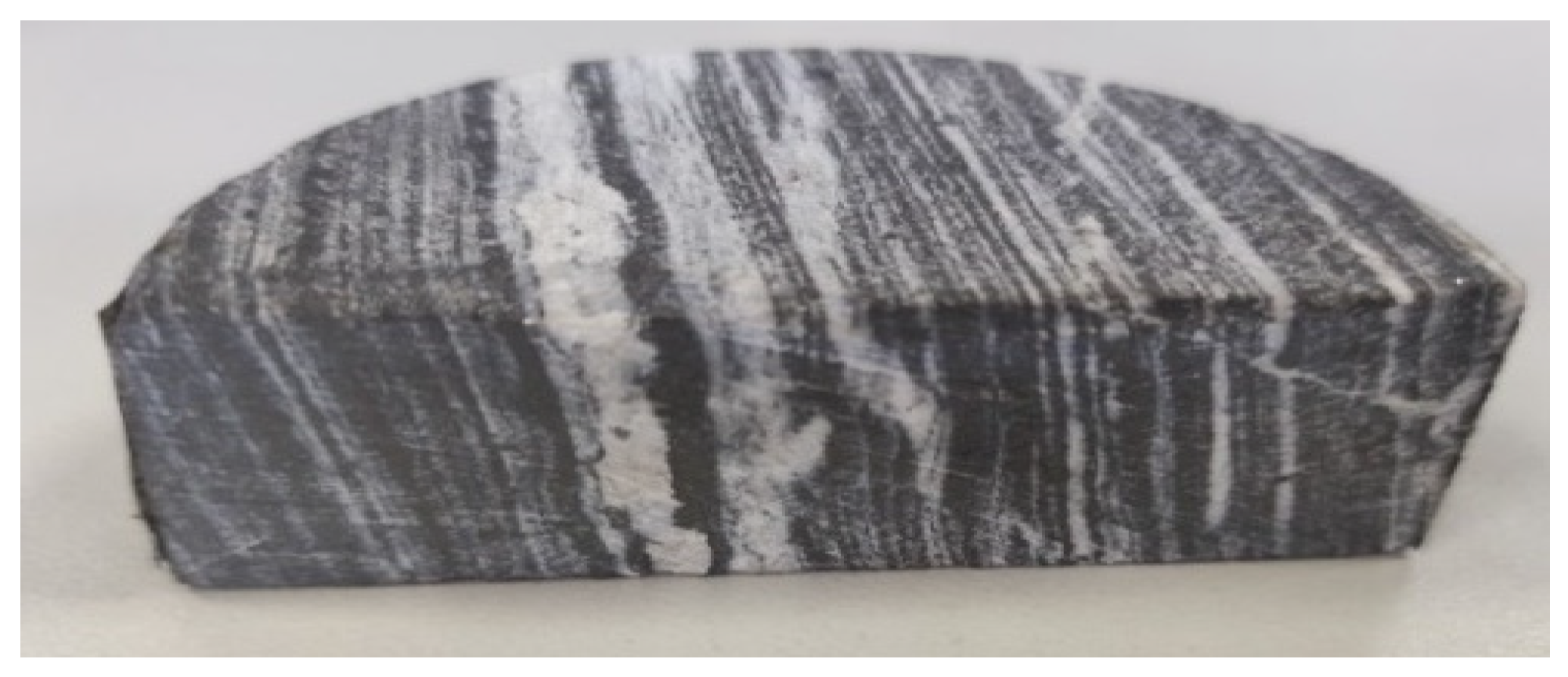
2.1. Iron Ore Sample Preparation

The BIF-hosted iron ore deposits in the Anshan–Benxi iron cluster of northeast China were selected as the study area. The region contains the largest banded iron ore in China, with iron ore reserves accounting for approximately 20% of China’s total iron ore reserves. The mineral composition in BIF-hosted iron ore has a distinctive black and white banding configuration (Figure 1). The black bands consist mainly of magnetite and hematite, while the white bands consist mainly of quartz [37].

Eleven disc-shaped experimental ore samples, each with a thickness of 1 cm and a diameter of 6 cm, were obtained by cutting ore samples collected from the open pit quarries in the study area. Single mineral samples (quartz, magnetite, and hematite) were collected simultaneously. The single mineral samples were procured from open-pit mines in the Anshan–Benxi region of Liaoning Province, China, and their purities were all above 95%.

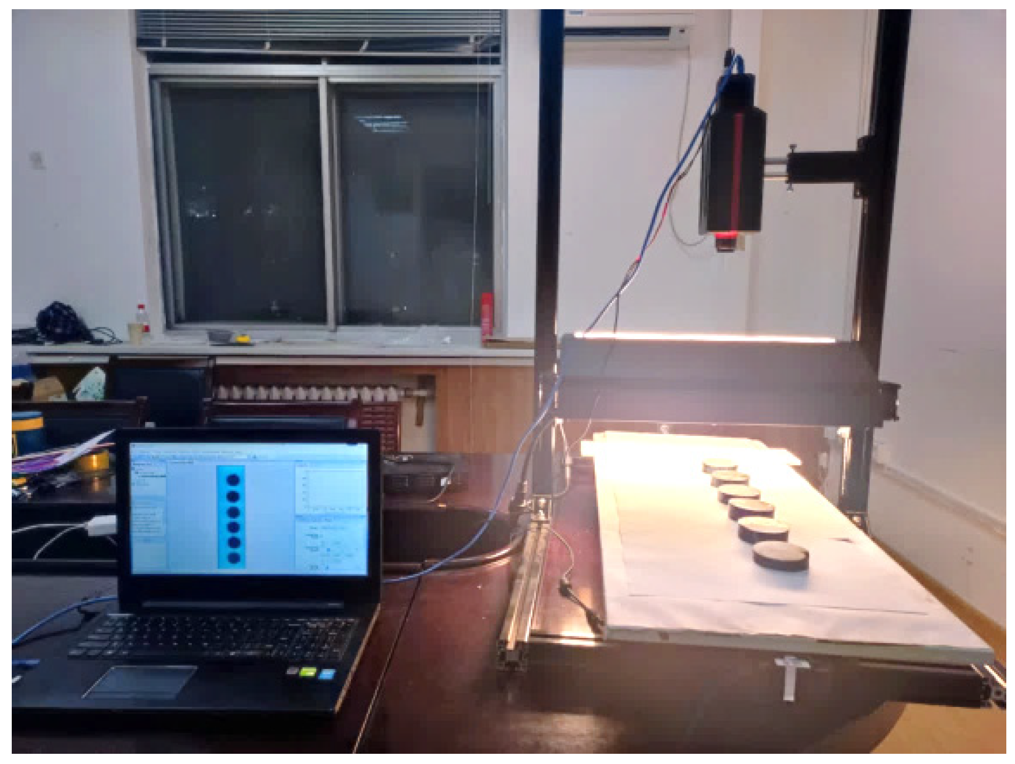
2.2. Hyperspectral Imaging System

The image data for the sample were obtained using the Resonon hyperspectral imaging system (Figure 2). The system was mainly composed of a hyperspectral camera, light source, displacement platform, and computer. Two kinds of hyperspectral cameras were used: PIka L and PIka IR-320 (Resonon, Inc., Bozeman, MT, USA). The wavelength ranges of the cameras were 400–1000 nm and 900–1700 nm, respectively, and the main technical parameters are shown in

Table 1. Main technical parameters of hyperspectral camera.

Parameters	PIka L	PIka NIR-320
Spectral range (nm)	400–1000	900–1700
Spectral resolution (nm)	2.1	4.9
Sampling interval (nm)	1.07	4.9
Spectral channels	561	164
Spatial channels	900	320
Pixel size (µm)	5.86	30

. The light source was a 150 W halogen lamp, which can provide spectral information in the range of 380–2000 nm. The displacement platform adopted the electronically controlled linear moving platform to realize the precise control of the sample displacement. The computer was mainly used for hyperspectral imaging system control and subsequent image data processing.

2.3. Hyperspectral Data Acquisition

To eliminate the potential for external light interference, the experiment was conducted in a dark indoor environment. Prior to the commencement of data collection, the samples were arranged in a sequential order on the displacement platform, with a white standard plate (Lambertian) placed in position. To guarantee optimal imaging, the frame rate of the two cameras and the velocity of the platform were calibrated to 20 fps, 0.47 mm/s and 10 fps, 1.1 mm/s, respectively. As the displacement platform moves smoothly, the camera sequentially captures the image information of the whiteboard and the sample. The raw image data acquired by the camera is the pixel brightness value, which is expressed in digital numbers (DN). This value was used to determine the response coefficient of the spectrometer by comparing it to the DN value of the whiteboard. The DN value of the sample was then converted into spectral reflectance according to the response coefficient. In addition, the two cameras sequentially acquired different image parameters due to different technical parameters. The spatial resolution and spectral resolution of the images obtained by the PIka L camera were 90 μm and 2.1 nm, respectively, while the PIka IR-320 camera had a resolution of 280 μm and 4.9 nm, respectively.

2.4. Sample Mineral Composition Measurement

Once the spectroscopic testing of all samples had been completed, they were sent to the Chemical Analysis and Testing Center in Shenyang, Liaoning Province, China for compositional analysis using titrimetric analysis and X-ray fluorescence.

Table 2. Content of each composition of the samples.

Sample ID	SiO2 (%)	Fe3O4 (%)	Fe2O3 (%)	Total (%)
1	46.33	51.2	2.08	99.61
2	51.89	13.92	33.13	98.94
3	54.05	6.40	38.18	98.63
4	55.05	1.03	43.81	99.89
5	55.11	0.50	43.08	98.69
6	57.28	4.67	37.23	99.18
7	62.29	7.41	29.85	99.55
8	62.28	1.10	36.15	99.53
9	64.02	4.99	30.16	99.17
10	64.80	0.87	32.11	98.78
11	53.27	12.04	34.46	99.77

displays the composition test results, which indicate that the samples were primarily composed of SiO₂, Fe₂O₃, and Fe₃O₄. The total amount of these three compositions was close to 100%.

3. Inversion Model Construction

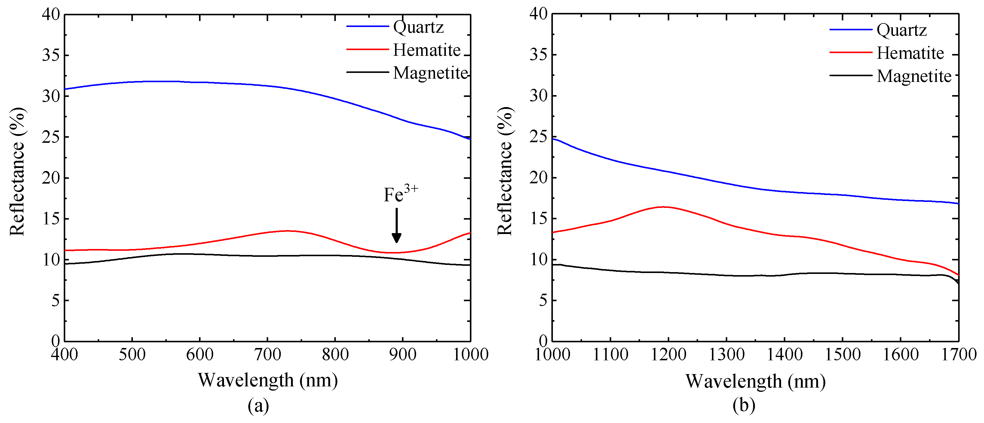
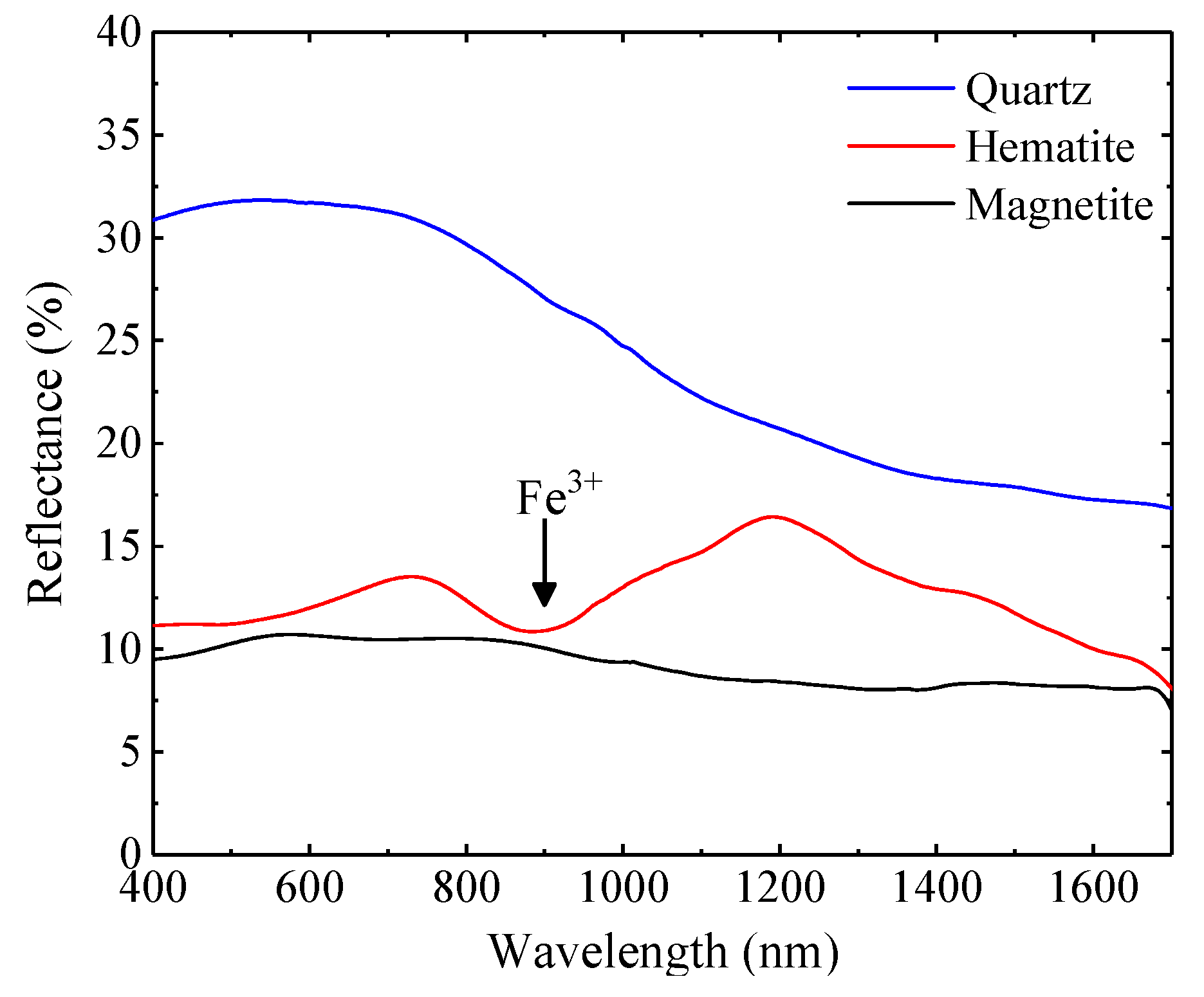
3.1. Mineral Reference Spectroscopy

In order to ensure the accurate identification of each mineral constituent within the sample, the spectra of three pure minerals (quartz, hematite, and magnetite) were employed as standard spectra. Figure 3 illustrates the outcomes of spectral analysis conducted on three pure minerals (quartz, hematite, and magnetite) using the Pika L and Pika NIR-320 hyperspectral imagers.

In order to obtain a comprehensive representation of the spectral characteristics of the minerals, the spectral data of VNIR and SWIR wavelength ranges were spliced, as shown in Figure 4.

Figure 4 illustrates the outcomes of the splicing of the quartz, hematite, and magnetite spectral data. A comparative analysis of the spectral characteristics of the three minerals revealed significant differences in the reflectance spectra of quartz, hematite, and magnetite.

Quartz: the spectral amplitude (spectral reflectivity) of quartz is significantly higher than that of hematite and magnetite in the range of 400–1700 nm. The average values of the spectral amplitude of quartz, hematite, and magnetite are 23.21%, 12.32%, and 9.26%, respectively. This is due to the differences in the absorption coefficients of quartz, hematite, and magnetite [38,39]. Quartz exhibits a comparatively weaker capacity to absorb light, giving rise to a higher spectral amplitude. In contrast, hematite and magnetite contain significant quantities of iron ions and exhibit a pronounced capacity to absorb light, resulting in a relatively low spectral amplitude. Furthermore, quartz does not exhibit discernible diagnostic absorption features within the visible wavelength band. This is attributed to the fact that quartz is an inorganic nonmetallic material with a relatively wide band gap, which renders the photon energy insufficient to excite the electrons in quartz to transition from the valence band to the conduction band [40]. In the near-infrared wavelength range, the reflectivity of quartz gradually decreases. This is attributed to the fact that the absorption of light by quartz increases with increasing wavelength.

Hematite: compared with quartz and magnetite, the most prominent spectral feature of hematite is the formation of a characteristic spectral band of strong reflection valleys with 750 nm as the left shoulder, 1200 nm as the right shoulder, and 900 nm as the valley. This phenomenon can be attributed to the electron transitions of Fe³⁺ in hematite, which gives rise to the formation of a pronounced spectral absorption peak around 900 nm in its spectral curve [25].

Magnetite: the spectral amplitude of magnetite is low across all bands, with values ranging from 8.06% to 10.71%. Additionally, the spectral curve is flat with little fluctuation. This phenomenon can be attributed to the high extinction of magnetite, which gives rise to a relatively flat reflectance spectrum [41,42].

In summary, the reflectance spectral amplitude of quartz is significantly higher than that of hematite and magnetite, while the spectral shape characteristics of hematite and magnetite differ significantly.

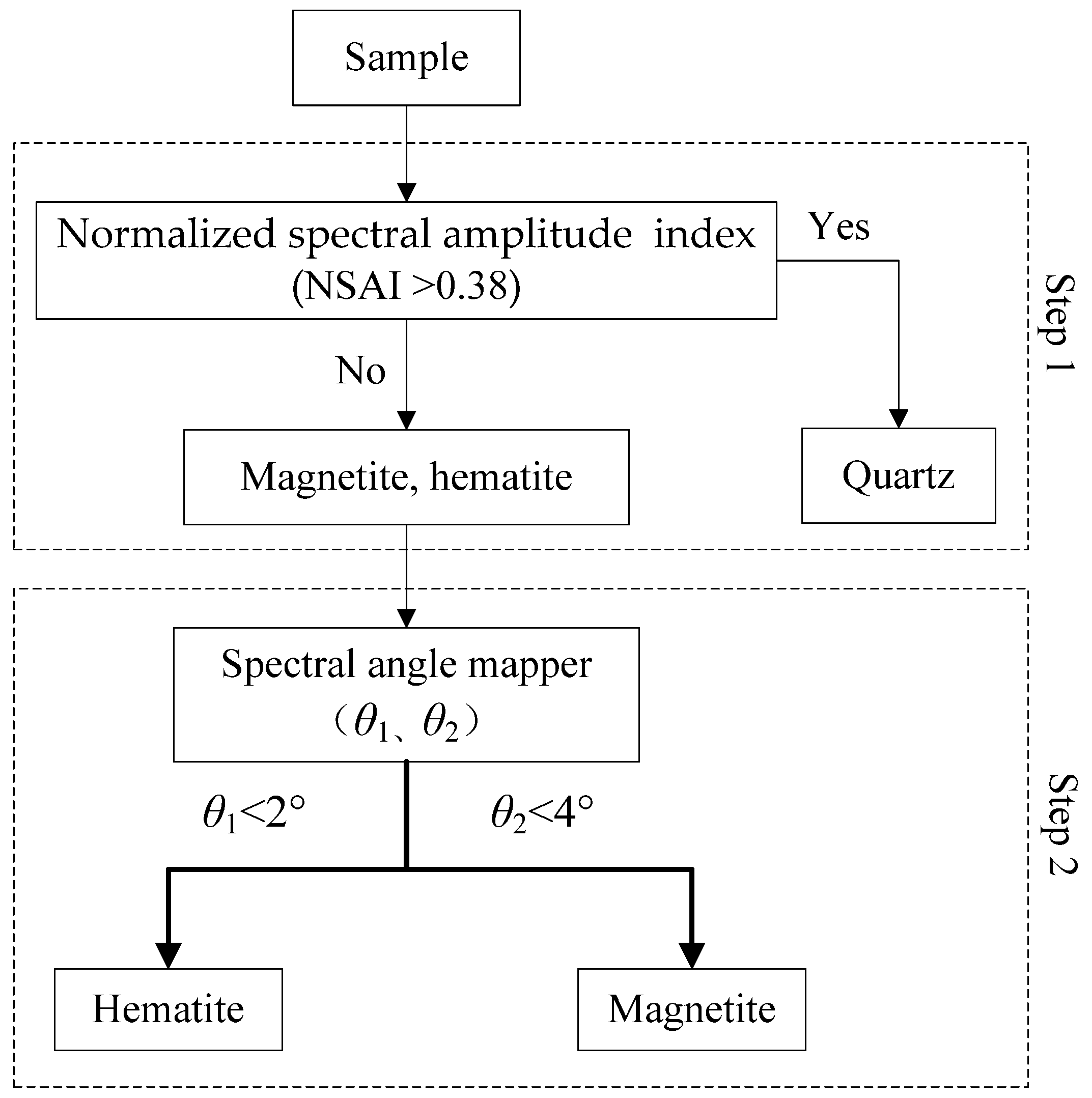
3.2. Model Construction

Given the limited number of experimental samples and the intricate intergrowth relationship between hematite and magnetite in the iron ore samples, the application of machine learning and spectral unmixing methods is not feasible for this experiment. Therefore, spectral index and spectral matching methods were chosen to construct identification models for quartz, hematite, and magnetite. The specific steps for building the model are as follows:

Step 1: identification of quartz.

In Figure 3a, the spectral amplitude of quartz is markedly higher than that of hematite and magnetite in the range of 400–1000 nm. Furthermore, the BIF-hosted iron ore samples are composed predominantly of quartz, hematite, and magnetite, with the three elements collectively representing nearly 100% of the sample (Table 2). Therefore, the identification model of quartz minerals in the BIF-hosted iron ore samples can be established based on the high amplitude characteristics of quartz spectra. Given that alterations in experimental conditions influence the strength of the spectral signals, the measured spectral data were initially normalized to enhance the stability of the spectral data, as shown in Equation (1).

$$R^{\prime }={\displaystyle \frac{R-R_{\min }}{R_{\max }-R_{\min }}}$$

(1)

where R is the initial spectral reflectance, R′ is the normalized spectral reflectance, and R_max and R_min are the maximum and minimum values of the spectral reflectance, respectively.

Subsequently, the normalized spectral amplitude index (NSAI) was constructed on the basis of the differences in the normalized spectral reflectance amplitude of different minerals, as shown in Equation (2).

$$NSAI={\displaystyle \sum _{i=1}^n{R}_i^{\prime }}/n$$

(2)

where R′ is the normalized spectral reflectance of the sample and n is the number of bands.

Calculated from Equation (2), the NSAIs of quartz, hematite, and magnetite in the range of 400–1000 nm were 0.93, 0.07, and 0.04, respectively. The threshold value was finally determined to be 0.38 after several attempts. That is, when the mineral’s NSAI value was greater than 0.38, it was classified as quartz, and when it was lower than 0.38, it was classified as hematite or magnetite.

Step 2: identification of hematite and magnetite.

Method Ⅰ: normalized difference iron index.

In Figure 3b, the spectral reflectance of hematite shows a clear increasing trend in the range of 1000–1150 nm, while magnetite shows a decreasing trend. Referring to the literature [43], the normalized difference iron index (NDII) was constructed to distinguish between hematite and magnetite, as shown in Equation (3):

$$NDII={\displaystyle \frac{R_{1150}-R_{1000}}{R_{1150}+R_{1000}}}$$

(3)

where R₁₁₅₀ and R₉₇₀ are the spectral reflectance of the sample at 1150 nm and 1000 nm, respectively. The NDII value of hematite was greater than 0, while the NDII value of magnetite was lower than 0.

Method Ⅱ: spectral angle mapper.

In Figure 3b, the difference in spectral shape characteristics between hematite and magnetite is obvious in the range of 1000–1700 nm. The two can be differentiated using the spectral angle mapper (SAM) [44] method, as shown in Equation (4):

$$\theta =arccos{\displaystyle \frac{{\displaystyle \sum _{i=1}^n{x}_i{y}_i}}{\sqrt{{\displaystyle \sum _{i=1}^n{x}_i^2}{\displaystyle \sum _{i=1}^n{y}_i^2}}}}\theta \in \left[0,90^o\right]$$

(4)

where $\theta$ is the angle between the reference spectrum $x_n$ and the unknown spectrum $y_n$ and $n$ is the number of bands.

Since a smaller spectral angle represents a higher degree of similarity between the reference and unknown spectra, the discrimination thresholds for the spectral angle (the angle between mineral spectral vectors) of hematite and magnetite were finally taken as 2° and 4°, respectively. When the angle ${\theta }_1$ between the unknown spectrum and the reference spectrum of hematite was lower than 2°, it was classified as hematite; when the angle ${\theta }_2$ between the unknown spectrum and the reference spectrum of magnetite was lower than 4°, it was classified as hematite.

After comparison, the SAM was found to be more effective than the NDII in differentiating hematite and magnetite. Therefore, the SAM model was chosen to identify hematite and magnetite.

To summarize, identifying the mineral composition of iron ore involved two steps. Firstly, the NSAI method was used to distinguish quartz from iron oxide minerals (hematite and magnetite) in the range of 400–1000 nm. Secondly, the SAM method was used to distinguish between hematite and magnetite in the range of 1000–1700 nm. Figure 5 illustrates the flow of the method to identify the spatial distribution of minerals in BIF-hosted iron ores by imaging spectrometer.

3.3. Model Evaluation Index

In order to evaluate the accuracy of the model, the mean absolute error (MAE) and root mean square error (RMSE) were selected as the statistical evaluation indexes of the model. MAE is the average absolute error between the predicted value and the true value of the model. The calculation formula is as follows:

$$MAE={\displaystyle \frac{1}{n}}{\displaystyle \sum _{i=1}^n\left|x_i-y_i\right|}$$

(5)

where $x_i$ is the predicted values of the model, $y_i$ is the true value, and $n$ is the number of experimental samples.

A lower MAE value indicates a higher degree of accuracy of the model prediction. This indicator provides an average level of the model’s prediction error. However, as the index assigns equal weight to all errors, it is less sensitive to abnormal errors.

The RMSE index is the root mean square of the error between the predicted value and the true value of the model. The calculation formula is as follows:

$$RMSE=\sqrt{{\displaystyle \frac{1}{n}}{\displaystyle \sum _{i=1}^n{\left(x_i-y_i\right)}^2}}$$

(6)

A lower RMSE value indicates a higher degree of accuracy of the model prediction. The square term in the RMSE calculation amplifies the impact of anomaly errors, making it a useful metric for identifying outliers in the model.

4. Model Validation and Discussion

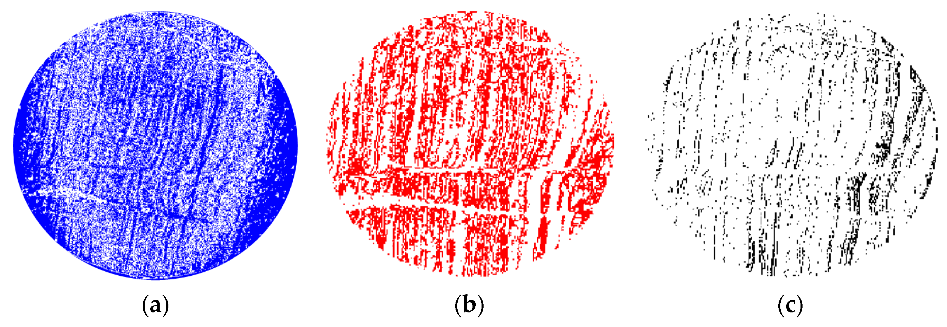
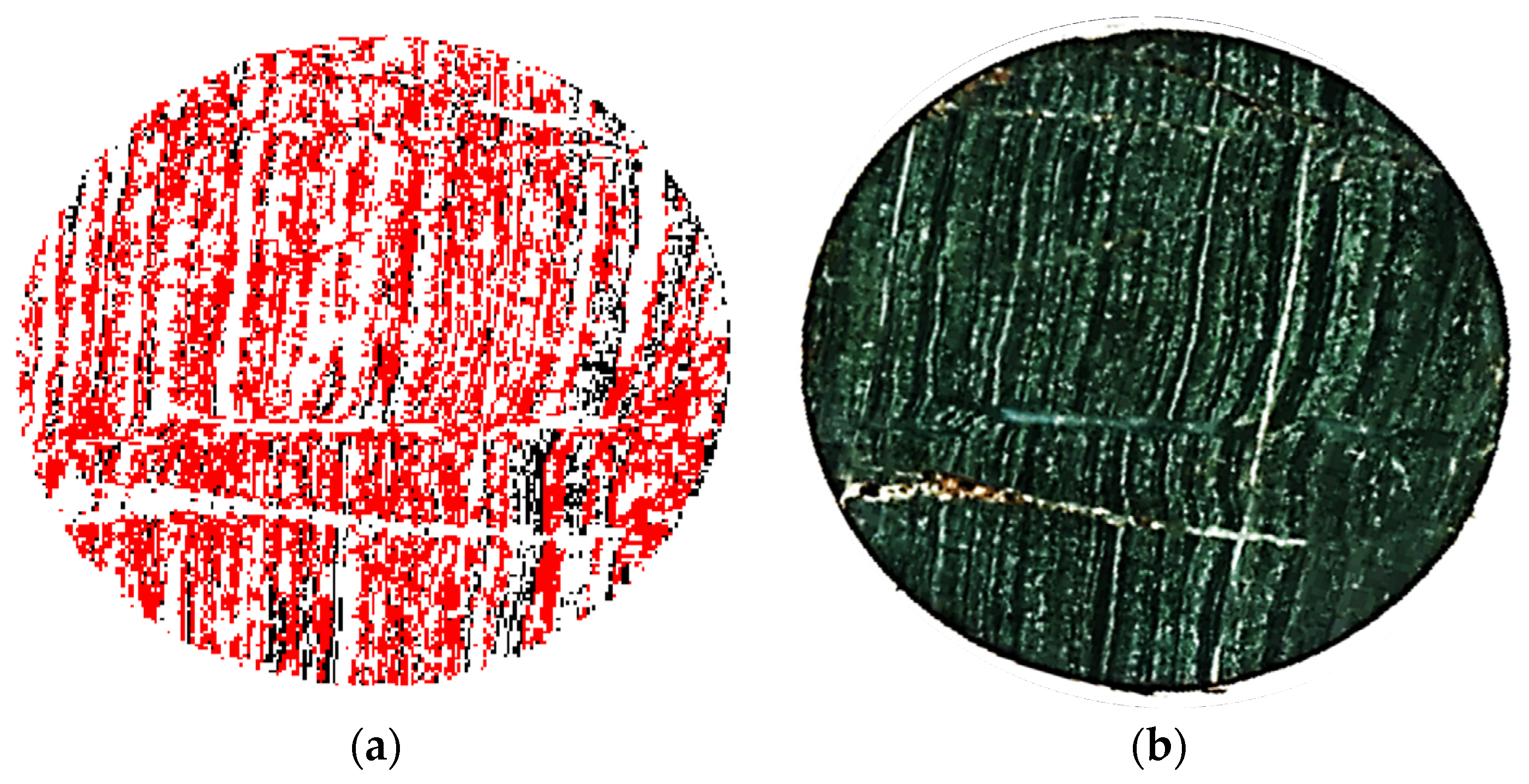
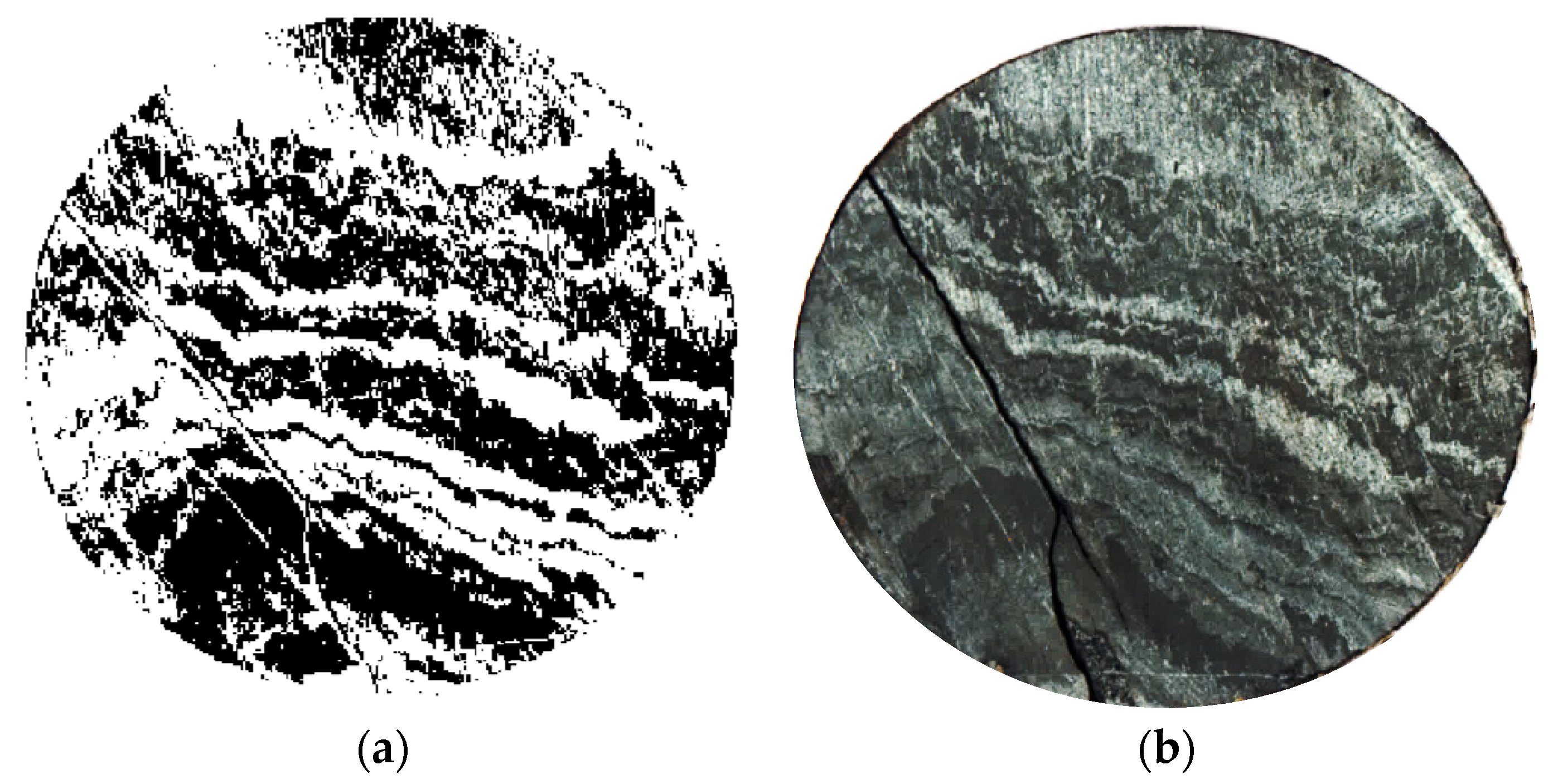
4.1. Identification Results of the Spatial Distribution of Iron Ore Components

The quartz, hematite, and magnetite of the 11 samples listed in Table 1 were identified using the above model. Due to the considerable number of samples, representative samples No. 3 and No. 1 were selected for presentation herein. Sample No. 3 displayed a higher concentration of hematite, reaching 38.18%, while sample No. 1 exhibited a higher concentration of magnetite, reaching 51.2%. The identification result of the hematite sample No. 3 is illustrated in Figure 6.

Figure 6a shows the high clarity quartz identification results obtained using a high spatial resolution spectrometer of 400–1000 nm. On the other hand, the results of hematite and magnetite identification using a low spatial resolution spectrometer of 1000–1700 nm, shown in Figure 6b,c, respectively, had relatively low clarity. Figure 7a displays the superimposed results of the identification of the three components, while Figure 7b is a visible light photograph of the same sample.

Furthermore, the results of the identification of sample No. 1, which had a relatively high magnetite content, are presented in Figure 8.

As illustrated in Figure 7 and Figure 8, the model’s identification of the spatial distribution of quartz, hematite, and magnetite in the two typical samples was largely consistent with the configuration of the sample strips. The identification effect was more satisfactory. The model was unable to identify the distribution of hematite in Figure 8a due to its extremely low content, which represented only 2.08% of the total sample.

4.2. Accuracy of Quantitative Inversion of Quartz, Hematite, and Magnetite

Due to the large size of the experimental samples, it was not possible to test the entire range of mineral distributions using microscope-type methods. Therefore, the microscope-type method could not be used to effectively test the identification potential of the model. To address this issue, an indirect method was used to examine the recognition effect of the model as follows.

First, the number of image elements of quartz, hematite, and magnetite within the lensing range was counted separately, based on the results of the model tests on the spatial distribution of the sample composition. In this way, the percentage of each of the three components at the sample surface could be obtained. Then, since the samples belonged to the strip structure and the mineral strips ran through their interior (see Figure 1), the percentages of the mineral compositions at the surface of the samples could be approximately equal to their volume fractions. Furthermore, the conversion equation between volume fraction and mass fraction can be expressed as follows:

$$m_i=v_i\times {\displaystyle \frac{{\rho }_i}{{\rho }_j}}$$

(7)

where $m_i$ and $v_i$ are the mass and volume fractions of the i-th mineral composition, ${\rho }_i$ is the density of the i-th mineral composition, and ${\rho }_j$ is the density of the j-th experimental sample. Where the sample density ${\rho }_j$ can be expressed as:

$${\rho }_j={\displaystyle \sum w_i\times {\rho }_i}$$

(8)

where $w_i$ is the mass fraction of the i-th mineral composition in the sample.

The densities of quartz, hematite, and magnetite were estimated at 2.71 g/cm³, 4.65 g/cm³, and 4.31 g/cm³, respectively. Therefore, the mass fractions of quartz, hematite, and magnetite in the samples could be obtained, and they were compared with the actual mass fractions of the sample’s compositions (see Table 2). The results are shown in

Table 3. Comparison of chemical test results with spectral test results.

Sample ID	Quartz(%)			Magnetite (%)			Hematite (%)
	True Value	Identified Value	Error	True Value	Identified Value	Error	True Value	Identified Value	Error
1	46.33	41.41	4.92	51.20	49.30	1.90	2.08	0.01	2.07
2	51.89	53.88	1.99	13.92	9.33	4.59	33.13	35.93	2.80
3	54.05	53.32	0.73	6.40	6.64	0.24	38.18	38.40	0.22
4	55.05	53.29	1.76	1.03	0.27	0.76	43.81	41.62	2.19
5	55.11	54.64	0.47	0.50	0.13	0.37	43.08	42.12	0.96
6	57.28	62.29	4.41	4.67	0.54	4.13	37.23	37.45	0.22
7	62.29	63.95	1.66	7.41	7.57	0.16	29.85	27.12	2.73
8	62.28	58.59	3.69	1.10	0.37	0.73	36.15	34.95	1.20
9	64.02	63.99	0.03	4.99	5.13	0.14	30.16	27.48	2.68
10	64.80	65.44	0.64	0.87	1.48	0.39	32.11	31.66	0.45
11	53.27	57.20	3.93	12.04	0.01	12.03	34.46	48.23	13.77

.

Table 3 shows that, with the exception of sample No. 11, the MAEs of the model for quartz, hematite, and magnetite identification were 2.03%, 1.34%, and 1.55%, respectively, and the RMSEs were 2.72%, 2.08%, and 1.85%, respectively. In terms of the fluctuation range of the error, hematite exhibited a smaller error fluctuation of 0.14%–2.80%, while quartz and magnetite exhibited a larger fluctuation range of 0.03%–4.92% and 0.14%–4.59%, respectively. The results demonstrate that the model exhibited high accuracy and stability. The reasons for the errors of sample No. 11 are analyzed below.

The magnetic susceptibilities (FeO/TFe) indicate the magnetic magnitude of iron ore [45]. Ore types are commonly categorized based on the magnitude of their magnetic susceptibilities into hematite, martite, and magnetite. Hematite, martite, and magnetite have magnetic susceptibilities of <28%, 28%–36%, and >36%, respectively. Upon testing sample No. 11, it was found that its magnetic rate was 29.93%, indicating that it belonged to martite. Martite is an ore that forms after the oxidation of magnetite [46]. It has the same composition as hematite, but maintains the crystalline form of magnetite. Therefore, the spectral curves of martite are similar to those of magnetite, resulting in the phenomenon of “different objects with the same spectrum” [47]. This led to the low accuracy of the model in recognizing martite. However, the iron oxide minerals in BIF-hosted iron ores are primarily magnetite and hematite [48], whereas the content of martite is minimal due to their more complex mineralization environment. Consequently, the model has substantial applicability potential. In order to identify martite, further studies may extend the range of the spectrum test from the visible–near-infrared band to the long-wave infrared (LWIR), with the objective of determining whether the emission spectrum characteristics of martite in the LWIR band differ from those of magnetite.

4.3. Discussion

It is worth noting that due to the influence of factors such as mineral composition, physical characteristics, and instrument resolution, the obtained spectral information inevitably exhibits errors and variations, both of which may eventually lead to the uncertainty of the experimental results. Therefore, the following aspects should be considered in future research.

The main mineral compositions of BIF-hosted iron ore sample are quartz, hematite, and magnetite. However, there is also a very small amount of martite associated with magnetite in the sample. Although the chemical composition of martite is identical to that of hematite, it retains the crystalline structure of magnetite, resulting in the spectral characteristics of martite being similar to those of magnetite. This phenomenon will lead to errors in the recognition results of the model. Subsequent experimental studies will be carried out on martite to further improve the accuracy of the model.

The surface roughness, porosity, and weathering degree of samples have an impact on the spectral characteristics of minerals, which, in turn, affects the spectral information of different samples. The aforementioned factors have the potential to introduce uncertainty into the recognition results of the model. Subsequent experimental studies should consider the impact of these factors on the spectral characteristics of the mineral.

Two types of hyperspectral cameras, PIka L and PIka NIL-320, were used in the experiment. The PIka NIL-320 camera exhibited a lower spatial resolution compared to the PIka L. Therefore, the pixel spectral information at the junction of different mineral bands of the sample may be aliasing, possibly affecting the accurate determination of mineral composition. With the development of hyperspectral imaging technology, higher resolution instruments will be used to verify the experimental results.

5. Conclusions

In this work, BIF-hosted iron ores were selected as experimental samples, and the test method for the spatial distribution of the sample composition was studied based on an imaging spectrometer. The following conclusions can be drawn from the study.

There are clear differences in the spectral amplitude and spectral shape characteristics of quartz, hematite, and magnetite in iron ores. A test model for the spatial distribution of iron ore components was developed based on this, using the normalized spectral amplitude index (NSAI) and spectral angle mapper (SAM). The spatial distribution of different minerals in the samples was tested using the model. The results demonstrated that, with the exception of one martite sample, the MAEs of the model for quartz, hematite, and magnetite were 2.03%, 1.34%, and 1.55%, respectively, and the RMSEs were 2.72%, 2.08%, and 1.85%, respectively. The model demonstrates a high degree of accuracy, and the test results of the spatial distribution of the three components are consistent with the banded tectonic character of the samples, indicating the method’s feasibility. This provides a new method for in situ testing of the spatial distribution of BIF-hosted iron ore components.

The influence of mineral crystal type gives rise to a phenomenon of “different objects with the same spectrum” between martite and magnetite. This renders the model ineffective in recognizing martite. Compared with the microscope method, the advantages of this method are simplicity, fast in-field operation, and wide application range. This method can not only identify the spatial distribution of minerals in BIF-hosted iron ore, but also test the species and abundance distribution of minerals in the drill core of other types of iron ore deposits. On the basis of the optimization and accuracy improvement of the model in the later stage, it is expected to be gradually applicable to mineral exploration, resource evaluation, and mineral processing.

References

1. Aftabi, A.; Atapour, H.; Mohseni, S.; Babaki, A. Geochemical discrimination among different types of banded iron formations (BIFs): A comparative review. Ore Geol. Rev. 2021, 136, 104244. [Google Scholar] [CrossRef]
2. Hassanzadeh, F.; Atapour, H.; Ranjbar, H. The Ediacaran metamorphosed banded iron formation (BIF) at Gohar Zamin mine (Gol-e-Gohar# 3 anomaly), Sirjan (southeastern Iran): Perspective from ore structures, bulk ore-rock geochemistry and OS-Pb isotopic signatures. Precambrian Res. 2023, 394, 107124. [Google Scholar]
3. Lv, Z.; Cheng, H.; Wei, M.; Zhao, D.; Wu, D.; Liu, C. Mineralogical characteristic and beneficiation evaluation of a Ta-Nb-Li-Rb deposit. Minerals 2022, 12, 457. [Google Scholar] [CrossRef]
4. Weibel, R.; Friis, H. Opaque minerals as keys for distinguishing oxidising and reducing diagenetic conditions in the Lower Triassic Bunter Sandstone, North German Basin. Sediment. Geol. 2004, 169, 129–149. [Google Scholar] [CrossRef]
5. Pabiś-Mazgaj, E.; Gawenda, T.; Pichniarczyk, P.; Stempkowska, A. Mineral composition and structural characterization of the clinoptilolite powders obtained from zeolite-rich tuffs. Minerals 2021, 11, 1030. [Google Scholar] [CrossRef]
6. Janovszky, P.; Jancsek, K.; Palásti, D.J.; Kopniczky, J.; Hopp, B.; Tóth, T.M.; Galbács, G. Classification of minerals and the assessment of lithium and beryllium content in granitoid rocks by laser-induced breakdown spectroscopy. J. Anal. At. Spectrom. 2021, 36, 813–823. [Google Scholar] [CrossRef]
7. El-Desoky, H.M.; Shebl, A.; Abdel-Rahman, A.M.; Fahmy, W.; El-Awny, H.; El-Sherif, A.M.; El-Rahmany, M.M.; Csámer, Á. Multiscale mineralogical investigations for mineral potentiality mapping of Ras El-Kharit-Wadi Khashir district, Southern Eastern Desert, Egypt. Egypt. J. Remote Sens. Space Sci. 2022, 25, 941–960. [Google Scholar] [CrossRef]
8. Xing, J.; Xian, H.; Yang, Y.; Chen, Q.; Xi, J.; Li, S.; He, H.; Zhu, J. Nanoscale Mineralogical Characterization of Terrestrial and Extraterrestrial Samples by Transmission Electron Microscopy: A Review. ACS Earth Space Chem. 2023, 7, 289–302. [Google Scholar] [CrossRef]
9. Pirard, E. Multispectral imaging of ore minerals in optical microscopy. Mineral. Mag. 2004, 68, 323–333. [Google Scholar] [CrossRef]
10. Tang, H.; Wang, H.; Wang, L.; Cao, C.; Nie, Y.; Liu, S. An Improved Mineral Image Recognition Method Based on Deep Learning. JOM 2023, 75, 2590–2602. [Google Scholar] [CrossRef]
11. Kuczyńska-Zemła, D.; Sundell, G.; Zemła, M.; Andersson, M.; Garbacz, H. The distribution of O and N in the surface region of laser-patterned titanium revealed by atom probe tomography. Appl. Surf. Sci. 2021, 562, 150193. [Google Scholar] [CrossRef]
12. Jeong, G.Y.; Nousiainen, T. TEM analysis of the internal structures and mineralogy of Asian dust particles and the implications for optical modeling. Atmos. Chem. Phys. 2014, 14, 7233–7254. [Google Scholar] [CrossRef]
13. Li, Y.; Deng, F.; Hall, T.; Goldys, E. M CRISPR/Cas12a-powered immunosensor suitable for ultra-sensitive whole Cryptosporidium oocyst detection from water samples using a plate reader. Water Res. 2021, 203, 117553. [Google Scholar] [CrossRef]
14. Abdullah; Ali, S.; Khan, Z.; Hussain, A.; Athar, A.; Kim, H.C. Computer vision based deep learning approach for the detection and classification of algae species using microscopic images. Water 2022, 14, 2219. [Google Scholar] [CrossRef]
15. Jain, U.; Saxena, K.; Chauhan, N. Helicobacter pylori induced reactive oxygen Species: A new and developing platform for detection. Helicobacter 2021, 26, e12796. [Google Scholar] [CrossRef] [PubMed]
16. Peyghambari, S.; Zhang, Y. Hyperspectral remote sensing in lithological mapping, mineral exploration, and environmental geology: An updated review. J. Appl. Remote Sens. 2021, 15, 031501. [Google Scholar] [CrossRef]
17. Lobo, A.; Garcia, E.; Barroso, G.; Martí, D.; Fernandez-Turiel, J.L.; Ibáñez-Insa, J. Machine Learning for Mineral Identification and Ore Estimation from Hyperspectral Imagery in Tin–Tungsten Deposits: Simulation under Indoor Conditions. Remote Sens. 2021, 13, 3258. [Google Scholar] [CrossRef]
18. Lorenz, S.; Ghamisi, P.; Kirsch, M.; Jackisch, R.; Rasti, B.; Gloaguen, R. Feature extraction for hyperspectral mineral domain mapping: A test of conventional and innovative methods. Remote Sens. Environ. 2021, 252, 112129. [Google Scholar] [CrossRef]
19. Shaik, I.; Begum, S.K.; Nagamani, P.V.; Kayet, N. Characterization and mapping of hematite ore mineral classes using hyperspectral remote sensing technique: A case study from Bailadila iron ore mining region. SN Appl. Sci. 2021, 3, 1–13. [Google Scholar] [CrossRef]
20. Duuring, P.; Hagemann, S.G.; Laukamp, C.; Chiarelli, L. Supergene modification of magnetite and hematite shear zones in banded iron-formation at Mt Richardson, Yilgarn Craton, Western Australia. Ore Geol. Rev. 2019, 111, 102995. [Google Scholar] [CrossRef]
21. De la Rosa, R.; Khodadadzadeh, M.; Tusa, L.; Kirsch, M.; Gisbert, G.; Tornos, F.; Tolosana-Delgado, R.; Gloaguen, R. Mineral quantification at deposit scale using drill-core hyperspectral data: A case study in the Iberian Pyrite Belt. Ore Geol. Rev. 2021, 139, 104514. [Google Scholar] [CrossRef]
22. Fouedjio, F.; Hill, E.J.; Laukamp, C. Geostatistical clustering as an aid for ore body domaining: Case study at the Rocklea Dome channel iron ore deposit, Western Australia. Appl. Earth Sci. 2018, 127, 15–29. [Google Scholar] [CrossRef]
23. Haest, M.; Cudahy, T.; Laukamp, C.; Gregory, S. Quantitative mineralogy from infrared spectroscopic data, I.I. Three-dimensional mineralogical characterization of the Rocklea channel iron deposit, Western Australia. Econ. Geol. 2012, 107, 229–249. [Google Scholar] [CrossRef]
24. Mathieu, M.; Roy, R.; Launeau, P.; Cathelineau, M.; Quirt, D. Alteration mapping on drill cores using a HySpex SWIR-320m hyperspectral camera: Application to the exploration of an unconformity-related uranium deposit (Saskatchewan, Canada). J. Geochem. Explor. 2017, 172, 71–88. [Google Scholar] [CrossRef]
25. Ramanaidou, E.; Wells, M.; Lau, I.; Laukamp, C. Characterization of iron ore by visible and infrared reflectance and, Raman spectroscopies. In Iron Ore; Woodhead Publishing: Cambridge, UK, 2015; pp. 191–228. [Google Scholar]
26. Zaini, N.; Van Der Meer, F.; Van Der Werff, H. Determination of Carbonate Rock Chemistry Using Laboratory-Based Hyperspectral Imagery. Remote Sens. 2014, 6, 4149–4172. [Google Scholar] [CrossRef]
27. Booysen, R.; Lorenz, S.; Thiele, S.T.; Fuchsloch, W.C.; Marais, T.; Nex, P.A.; Gloaguen, R. Accurate hyperspectral imaging of mineralised outcrops: An example from lithium-bearing pegmatites at Uis, Namibia. Remote Sens. Environ. 2022, 269, 112790. [Google Scholar] [CrossRef]
28. Hao, D.; Yao, Y.; Fu, J.; Michalski, J.R.; Song, K. The laboratory-based hyspex features of chlorite as the exploration tool for high-grade iron ore in Anshan-Benxi Area, Liaoning Province, Northeast China. Appl. Sci. 2020, 10, 7444. [Google Scholar] [CrossRef]
29. Mao, Y.; Ma, B.; Liu, S.; Wu, L.; Zhang, X.; Yu, M. Study and validation of a remote sensing model for coal extraction based on reflectance spectrum features. Can. J. Remote Sens. 2014, 40, 327–335. [Google Scholar] [CrossRef]
30. Kumar, C.; Chatterjee, S.; Oommen, T. Mapping hydrothermal alteration minerals using high-resolution AVIRIS-NG hyperspectral data in the Hutti-Maski gold deposit area, India. Int. J. Remote Sens. 2020, 41, 794–812. [Google Scholar] [CrossRef]
31. Shi, C.; Wang, L. Incorporating spatial information in spectral unmixing: A review. Remote Sens. Environ. 2014, 149, 70–87. [Google Scholar] [CrossRef]
32. Lussier, F.; Thibault, V.; Charron, B.; Wallace, G.Q.; Masson, J.F. Deep learning and artificial intelligence methods for Raman and surface-enhanced Raman scattering. TrAC Trends Anal. Chem. 2020, 124, 115796. [Google Scholar] [CrossRef]
33. Khushboo; Bala, N.; Rawat, S.; Singh, S.; Arya, R. A Study of Spectral Data Processing with Emphasis on Spectral Similarity Measures for Hyperspectral Image Processing. In Soft Computing: Theories and Applications: Proceedings of SoCTA 2018; Springer: Singapore, 2020; pp. 859–868. [Google Scholar]
34. Van der Meer, F. The effectiveness of spectral similarity measures for the analysis of hyperspectral imagery. Int. J. Appl. Earth Obs. Geoinf. 2006, 8, 3–17. [Google Scholar] [CrossRef]
35. Bakker, W.H.; Schmidt, K.S. Hyperspectral edge filtering for measuring homogeneity of surface cover types. ISPRS J. Photogramm. Remote Sens. 2002, 56, 246–256. [Google Scholar] [CrossRef]
36. Wang, K.; Yong, B.; Gu, X.; Xiao, P.; Zhang, X. Spectral similarity measure using frequency spectrum for hyperspectral image classification. IEEE Geosci. Remote Sens. Lett. 2014, 12, 130–134. [Google Scholar] [CrossRef]
37. Li, H.; Zhang, Z.; Li, L.; Zhang, Z.; Chen, J.; Yao, T. Types and general characteristics of the BIF-related iron deposits in China. Ore Geol. Rev. 2014, 57, 264–287. [Google Scholar] [CrossRef]
38. Noda, S.; Yamaguchi, Y. Estimation of surface iron oxide abundance with suppression of grain size and topography effects. Ore Geol. Rev. 2017, 83, 312–320. [Google Scholar] [CrossRef]
39. Cudahy, T.J.; Ramanaidou, E.R. Measurement of the hematite: Goethite ratio using field visible and near-infrared reflectance spectrometry in channel iron deposits. West. Australia. Aust. J. Earth Sci. 1997, 44, 411–420. [Google Scholar] [CrossRef]
40. Fisher, A.J.; Hayes, W.; Stoneham, A.M. Theory of the structure of the self-trapped exciton in quartz. J. Phys. Condens. Matter. 1990, 2, 6707. [Google Scholar] [CrossRef]
41. Izawa MR, M.; Cloutis, E.A.; Rhind, T.; Mertzman, S.A.; Applin, D.M.; Stromberg, J.M.; Sherman, D.M. Spectral reflectance properties of magnetites: Implications for remote sensing. Icarus 2019, 319, 525–539. [Google Scholar] [CrossRef]
42. Hunt, G.R. Visible and near-infrared spectra of minerals and rocks: III. Oxides and hydro-oxides. Mod. Geol. 1971, 2, 195–205. [Google Scholar]
43. Mao, Y.; Wang, D.; Liu, S.; Song, L.; Wang, Y.; Zhao, Z. Research and verification of a remote sensing BIF model based on spectral reflectance characteristics. J. Indian Soc. Remote Sens. 2019, 47, 1051–1061. [Google Scholar] [CrossRef]
44. Sinaice, B.B.; Owada, N.; Ikeda, H.; Toriya, H.; Bagai, Z.; Shemang, E.; Adachi, T.; Kawamura, Y. Spectral angle mapping and AI methods applied in automatic identification of Placer deposit magnetite using multispectral camera mounted on UAV. Minerals 2022, 12, 268. [Google Scholar] [CrossRef]
45. Zhang, H.; Zhang, P.; Zhou, F.; Lu, M. Application of multi-stage dynamic magnetizing roasting technology on the utilization of cryptocrystalline oolitic hematite: A review. Int. J. Min. Sci. Technol. 2022, 32, 865–876. [Google Scholar] [CrossRef]
46. Zhu, D.; Jiang, Y.; Pan, J.; Yang, C. Study of Mineralogy and Metallurgical Properties of Lump Ores. Metals 2022, 12, 1805. [Google Scholar] [CrossRef]
47. Song, L.; Liu, S.J.; Yu, M.L.; Mao, Y.C.; Wu, L.X. A classification method based on the combination of visible, near-infrared and thermal infrared spectrum for coal and gangue distinguishment. Guang Pu Xue Yu Guang Pu Fen Xi = Guang Pu. 2017, 37, 416–422. [Google Scholar]
48. Moon, I.; Lee, I.; Seo, J.H.; Yang, X. Geochemical studies of banded iron formations (BIFs) in the North China Craton: A review. Geosci. J. 2017, 21, 971–983. [Google Scholar] [CrossRef]
Figure 1. Banded structure of BIF-hosted iron ore.
Minerals 14 00959 g001
Figure 2. Hyperspectral imaging system.
Minerals 14 00959 g002
Figure 3. Reflectance spectra of quartz, magnetite, and hematite. (a) Visible–Near Infrared (VNIR: 400–1000 nm); (b) shortwave-infrared (SWIR: 1000–1700 nm).
Minerals 14 00959 g003
Figure 4. Reflectance spectra of quartz, magnetite, and hematite at different wavelengths in the range of 400–1700 nm.
Minerals 14 00959 g004
Figure 5. Sample composition identification process.
Minerals 14 00959 g005
Figure 6. Identification results of the mineral distribution of a sample. (a) Quartz—white; (b) hematite—red; (c) magnetite—black.
Minerals 14 00959 g006
Figure 7. The recognition results of the model were compared with the visible light photos of sample No. 3. (a) Recognition results of different mineral fractions. Quartz—white, hematite—red, magnetite—black. (b) Visible light photo of the sample surface.
Minerals 14 00959 g007
Figure 8. The recognition results of the model were compared with the visible light photos of the sample No. 1. (a) Recognition results of different mineral fractions. Quartz—white, magnetite—black. (b) Visible light photo of the sample surface.
Minerals 14 00959 g008