A Least Squares Estimator for Gradual Change-Point in Time Series with m-Asymptotically Almost Negatively Associated Errors

Abstract

As a new member of the NA (negative associated) family, the m-AANA (m-asymptotically almost negatively associated) sequence has many statistical properties that have not been developed. This paper mainly studies its properties in the gradual change point model. Firstly, we propose a least squares type change point estimator, then derive the convergence rates and consistency of the estimator, and provide the limit distributions of the estimator. It is interesting that the convergence rates of the estimator are the same as that of the change point estimator for independent identically distributed observations. Finally, the effectiveness of the estimator in limited samples can be verified through several sets of simulation experiments and an actual hydrological example.

1. Introduction

Change point problems originally arose from quality control engineering [1]. Because of the heterogeneities in real data sequences, the problems of change point estimation and detection in real data sequences have drawn attention. Scholars have proposed many methods to solve various data problems (see [2,3,4,5,6,7,8,9]). The purpose of change point detection and estimation is to divide a data sequence into several homogeneous segments, and the theories have been applied in many fields like finance [10], medicine [11], environment [12] and so on. For some special problems, such as hydrological and meteorological problems, most of the change point that occur are gradual rather than abrupt. Therefore, the research on the problems of gradual change is very meaningful.

In earlier research, most theories of gradual changes were derived from two-stage regression model [13,14]. Hušková [15] used the least–squares method to estimate an unknown gradual change point and the model is as follows:

For $n>1$, observations $X_1$, $X_2$, ⋯, $X_n$ shall satisfy:

$$X_t=\mu +\delta {\left(\frac{i-m}{n}\right)}_{+}+e_i,1\le i\le n,$$

where ${\left(a\right)}_{+}=max(0,a)$, $\mu ,\delta \ne 0$, m is the location of the change, $e_1,e_2,\cdots ,e_n$ are i.i.d. random variables with $E{e}_i=0$, $var\left(e_i\right)={\sigma }^2$, $E|e_i{|}^{2+\Delta }<\infty$ for some $\Delta >0$. In the same year, Jarušková [16] conducted a log likelihood ratio test of the model on the basis of Hušková [15], and obtained that the asymptotic distribution of the test statistic is Gumbel distribution.

Later, Wang [17] extended the error terms $e_i$ from the traditional i.i.d. sequences to the long memory i.i.d sequences and obtained the consistency of the estimator of the mean gradual change point and the limit distribution of the test statistic. Then, Timmermann [18] tested the gradual change in general random processes and update processes respectively, and also obtained the limit distribution of test statistic. It is well known that most of the previous studies tend to focus on the abrupt change. But for some important time series, such as temperature and hydrology, there is a greater possibility of gradual mean change.

Therefore, this paper considers the gradual change problem and the following model based on Hušková [15] is constructed:

$$X_t=\mu +{\delta }_n{\left(\frac{t-k^{*}}{n}\right)}_{+}^{\gamma }+Y_t,1\le t\le n,$$

(1)

where $n>1$, $X_1$, $X_2$, ⋯, $X_n$ are observations. ${\left(a\right)}_{+}=max(0,a)$, $\gamma \in (0,1)$, and $k^{*}$ is unknow change point location. $\mu$, ${\delta }_n$ are unknown parameter, $\mu ,{\delta }_n\ne 0$ with $\frac{n^{1/2}\left|{\delta }_n\right|}{{(logn)}^{1/2}}\to \infty$. $Y_1,Y_2,\cdots ,Y_n$ are random variables with zero mean.

The least squares method is a classic method (see [19,20]). In model (1), the estimators of $k^{*}$ and ${\tau }^{*}$ based on the least–squares–type are, respectively:

$${\widehat{k}}^{*}=min\left\{k:k=arg\underset{j}{max}{U}_j\left(\gamma \right);j=1,2,\cdots ,n-1\right\},$$

(2)

$${\widehat{\tau }}^{*}={\widehat{k}}^{*}/n,$$

(3)

where:

$$U_j\left(\gamma \right)=\frac{\left|{\sum }_{t=1}^n(x_{tj}-{\overline{x}}_j)X_t\right|}{{\left({\sum }_{t=1}^n{(x_{tj}-{\overline{x}}_j)}^2\right)}^{1/2}}.$$

(4)

For convenience of illustration, $x_{tj}$ and ${\overline{x}}_j$ are ${\left(\frac{t-j}{n}\right)}_{+}^{\gamma }$ and $\frac{1}{n}\sum _{t=1}^n{x}_{tj}$, respectively.

It can be seen that most previous studies have one thing in common, namely that the error terms are independently and identically distributed. However, the constraints of independent sequences are quite strict, and in practical problems, many time series models may not meet the independent conditions. This leads to a classical question of whether the error terms in a model can be generalized to some more general cases. Therefore, the idea of extending the error terms to the m-AANA sequences is proposed in this paper. Before presenting the main asymptotic results, it is necessary to understand the following definition:

Definition 1 ([21]).

There is an fixed integer $m\ge 1$, the random variable sequence $\{Y_n,n\ge 1\}$ is called m-AANA sequence if there exists a non negative sequence $q\left(n\right)\to 0$ as $n\to \infty$ such that:

$$Cov\{f\left(Y_n\right),g(Y_{n+m},\cdots ,Y_{n+k})\}\le q\left(n\right){\left[Var\left(f\left(Y_n\right)\right)Var\left(g(Y_{n+m},\cdots ,Y_{n+k})\right)\right]}^{1/2},$$

(5)

for all $n\ge 1$, $k\ge m$ and for all coordinatewise nondecreasing continuous functions f and g whenever the variances exist. The sequence $\left\{q\right(n),n\ge 1\}$ is called the mixing coefficients of $\{Y_n,n\ge 1\}$. It is not difficult to see that NA family includes NA [22], m-NA [23], AANA [24], and independent sequences.

Scholars have great interest in the sequences of NA family. For example, NA sequence is opposite to PA (positively associated) sequence, but NA sequence has better property than other existing ND (negatively dependent) sequence: under the influence of increasing functions, the disjoint subset of NA random variable sequence is still NA. Therefore, NA sequences appeared in many literary works. Przemysaw [25] obtained the convergence of partial sums of NA sequences; Yang [26] obtained Bernstein type inequalities for NA sequences; and Cai [27] obtained the Marcinkiewicz – Zygmund type strong law of large numbers of NA sequences.

There are many classical studies about m-NA and AANA sequences as generalizations of NA sequences. Hu [23] discussed the complete convergence of m-NA sequences; Yuan [28] proposed a Marcinkiewics-Zygmund type moment inequality for the maximum partial sum of AANA sequences.

For the m-AANA sequence mentioned in this paper, it is a relatively new concept and its research results are less than those of other sequences in NA family. Ko [29] extended Hájek–Rényi inequalities and the strong law of large numbers of Nam [21] to Hilbert space; Ding [30] proposed the CUSUM method to estimate the abrupt change point in a sequence with the error term of m-AANA process, but for a more general case, he did not discuss the gradual change. Therefore, another reason for constructing the main ideas of this paper is is to fill the research gaps of Ding [30].

The rest is arranged as follows: Section 2 describes the main results. A small simulation study under different parameters and an example is provided in Section 3. Section 4 contains the conclusions and outlooks, and the main results are proved in Appendix A.

2. Main Results

For our asymptotic results, assume the model to satisfy the following assumptions:

Assumption 1.

$\{Y_n,n\ge 1\}$ is a sequence of m-AANA random variables with $E{Y}_n=0$, $E{Y}_n^2={\sigma }^2<\infty$, and there is a $v>0$, $E|Y_n{|}^{2+v}<\infty$.

Assumption 2.

The mixing coefficient sequence $\left\{q\right(n),n\ge 1\}$ satisfies ${\sum }_{n=1}^{\infty }q\left(n\right),$${\sum }_{n=1}^{\infty }{q}^2\left(n\right)<\infty$.

Assumption 3.

We note $S_{i,n}={\sum }_{j=1}^n{Y}_{j+i}$, $S_n=S_{0,n}$. As $n\to \infty$,

$$\frac{E{S}_n^2}{n}=s^2<\infty .$$

In addition, there exists strictly ascending sequence of natural numbers $\left\{n_k\right\}$ with $n_0=0$ and $m_i=n_i-n_{i-1}$. And for some $0<\alpha \le 1$, ${\sum }_{i=1}^{\infty }{\left(\frac{m_i}{n_i}\right)}^{1+\alpha /2}<\infty$, $\underset{i\to \infty }{lim}$$\frac{E{S}_{n_{i-1},m_i}^2}{m_i}=s^2<\infty$.

Remark 1.

Assumption 1 and 2 are the underlying assumptions, and if these assumptions cannot be met, serious problems such as bias in the estimates, inconsistency in the estimates, and invalidity of the estimates may arise in the proof process.

In addition, what can be verified is that the m-AANA random variables satisfy the central limit theorem when Assumption 1–3 are ture.

Let $\tau =k/n$, ${\tau }^{*}=k^{*}/n$, we obtain the Theorem 1.

Theorem 1.

If Assumption 1 and 2 are ture, when $n\to \infty$,

$$|{\widehat{\tau }}^{*}-{\tau }^{*}|=o_p\left(1\right).$$

Theorem 2.

If Theorem 1 holds, when $n\to \infty$,

$$|{\widehat{k}}^{*}-k^{*}|=O_p(▵),$$

$$▵=\left\{\begin{array}{cccc}\hfill & {\left({\delta }_n^{-2}{n}^{2\gamma }\right)}^{1/(2\gamma +1)},\hfill & \hfill & \gamma \in (0,1/2),\hfill \\ \hfill & {\delta }_n^{-1}{n}^{1/2}{(log(n-k^{*}))}^{-1/2},\hfill & \hfill & \gamma =1/2,\hfill \\ \hfill & {\delta }_n^{-1}{n}^{1/2},\hfill & \hfill & \gamma \in (1/2,1).\hfill \end{array}\right.$$

Remark 2.

Interestingly, these convergence rates are the same as those in Hušková [31], but independent sequences are contained in m-AANA sequences.

Theorem 3.

Case 1. Assuming that Assumption 1–3 hold true. If $\gamma \in (0,\frac{1}{2})$, as $n\to \infty$, then:

$${\left({\delta }_n^2{n}^{-2\gamma }\right)}^{1/(2\gamma +1)}({\widehat{k}}^{*}-k^{*})/({\sigma }^2-C_7)\stackrel{\mathcal{D}}{\to }{V}_{\gamma },$$

(6)

where $V_{\gamma }=argmax\left\{Z_{\gamma }\left(i\right)-{\int }_{-\infty }^{\infty }{({(x+i)}_{+}^{\gamma }-x_{+}^{\gamma })}^{2}dx/2;i\in R\right\}$ with $\left\{Z_{\gamma }\left(i\right);i\in R\right\}$ is a Gaussian process with zero mean and covariance function.

$$Cov(Z_{\gamma }\left(i\right),Z_{\gamma }\left(s\right))={\int }_{-\infty }^{\infty }({(x+i)}_{+}^{\gamma }-x_{+}^{\gamma })({(x+s)}_{+}^{\gamma }-x_{+}^{\gamma })dx,i,s\in R.$$

(7)

Case 2. Assuming that Assumption 1–3 hold true. If $\gamma =\frac{1}{2}$, as $n\to \infty$, then:

$$\frac{{\delta }_n{(log(n-k^{*}))}^{1/2}}{2n^{1/2}}\frac{{\widehat{k}}^{*}-k^{*}}{{({\sigma }^2-C_8)}^{1/2}}\stackrel{\mathcal{D}}{\to }{V}_{1/2}$$

(8)

where $V_{1/2}$ is a standard normal variable.

Case 3. Assuming that Assumption 1–3 hold true. If $\gamma \in (\frac{1}{2},1)$, as $n\to \infty$, then:

$$\frac{{\delta }_n}{n^{1/2}}\frac{{\widehat{k}}^{*}-k^{*}}{{({\sigma }^2-C_9)}^{1/2}}\stackrel{\mathcal{D}}{\to }{V}_{\gamma }^{{}^{\prime }}$$

(9)

where $V_{\gamma }^{{}^{\prime }}$ is a normal $N(0,g^{-2}({\tau }^{*},\gamma ))$ random variable with:

$$g^2({\tau }^{*},\gamma )={(1-{\tau }^{*})}^{(2\gamma -1)}\left\{\frac{2\gamma +1}{4}\frac{{(\gamma -1+2{\tau }^{*})}^2}{{\gamma }^2+{\tau }^{*}(1+2\gamma )}-\frac{1}{2\gamma -1}({(\gamma -1)}^2+{\tau }^{*}(2\gamma -1))\right\}.$$

(10)

$C_7,C_8,C_9<{\sigma }^2$ are constants and are described in the proofs in Appendix A.

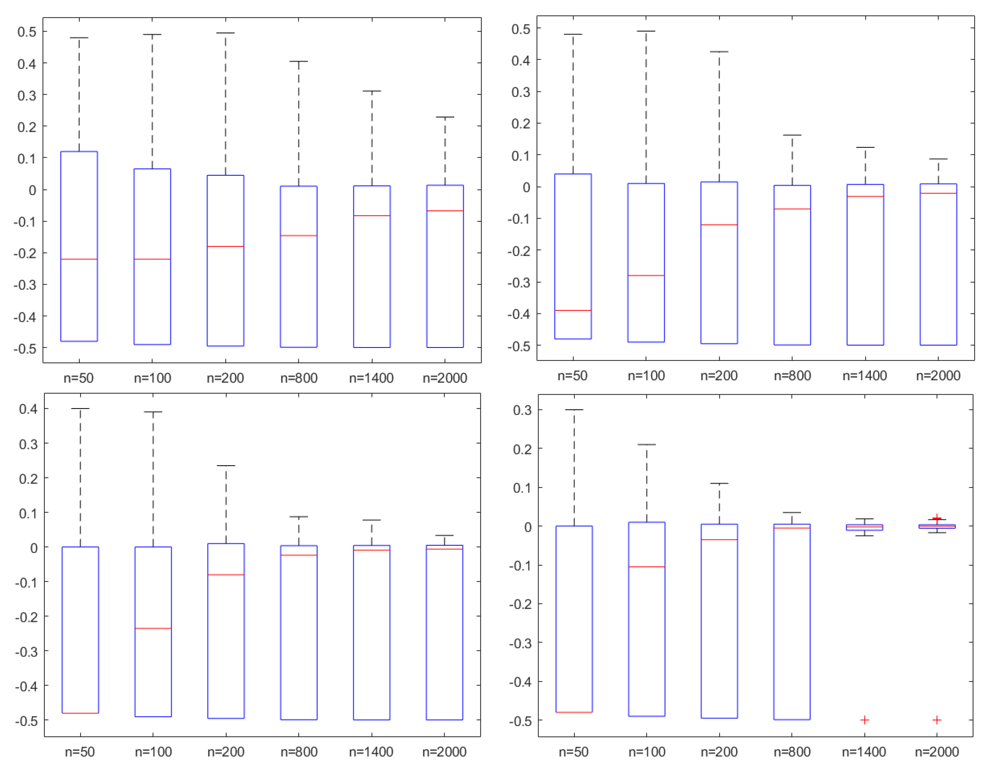
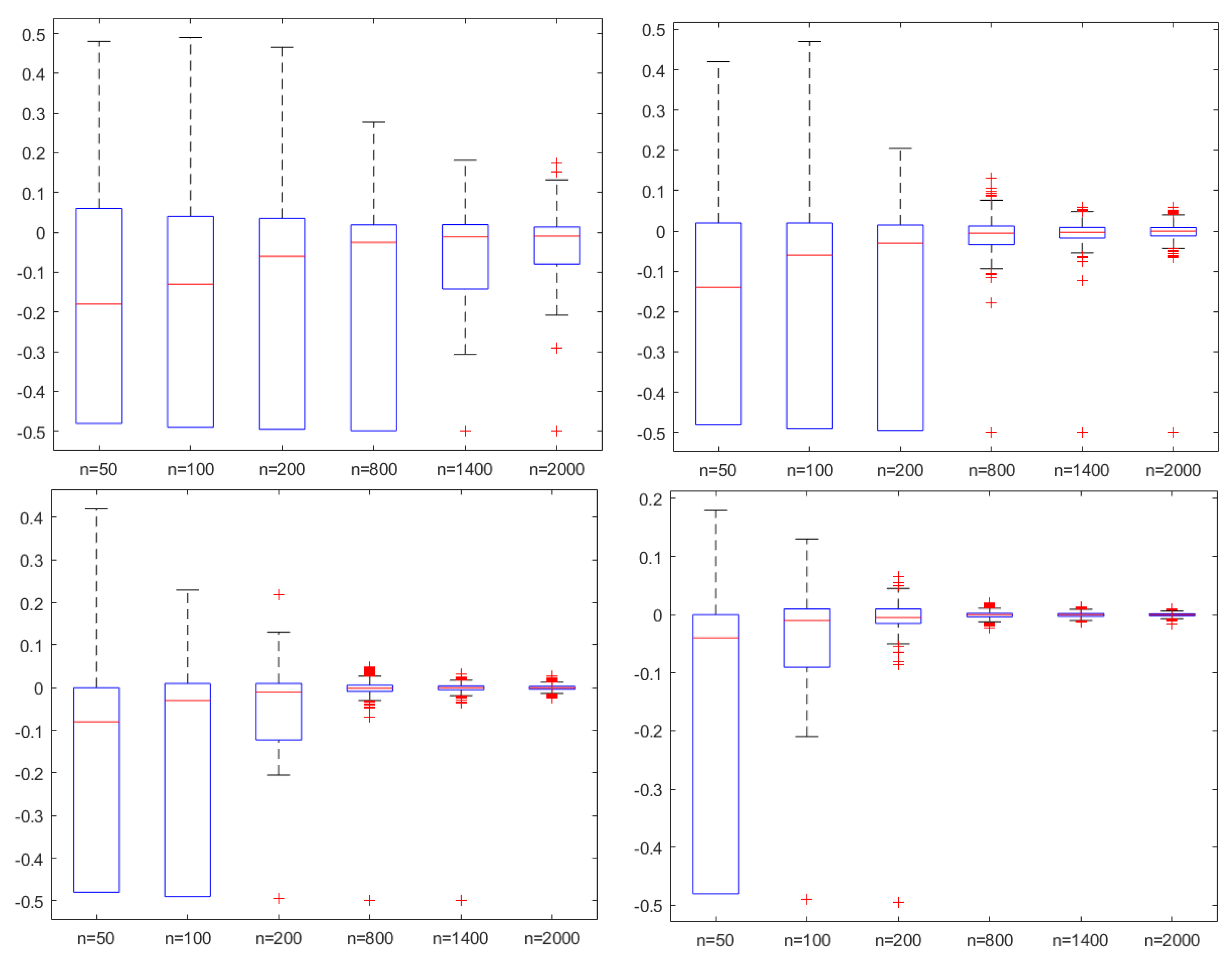
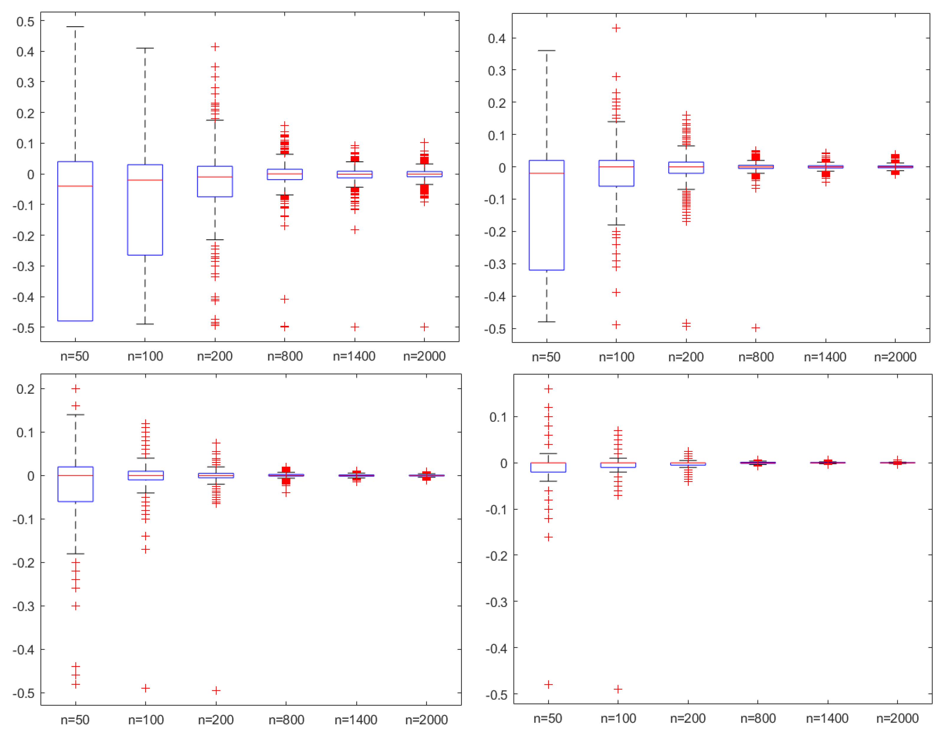
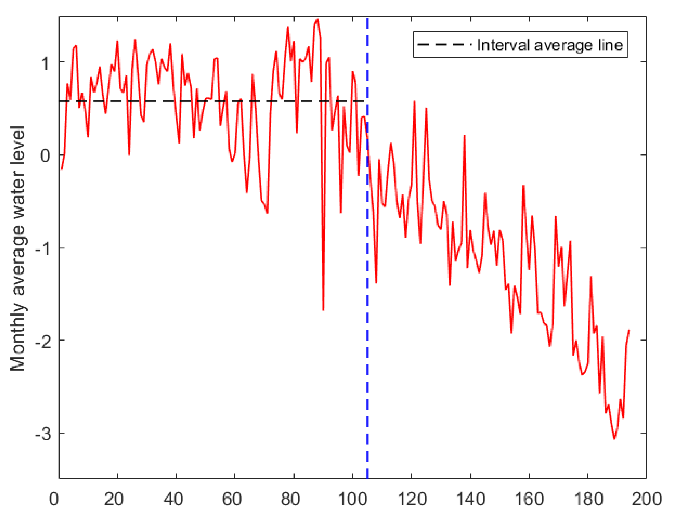
3. Simulations and Example

In this section, assume that there is only one gradual change point of mean at $k^{*}$ in (1), such that:

$$X_t=\mu +{\delta }_n{\left(\frac{t-k^{*}}{n}\right)}_{+}^{\gamma }+Y_t,1\le t\le n,$$

$Y_1,Y_2,\cdots ,Y_n$ satisfy:

$$(Y_1,Y_2,\cdots ,Y_n)\stackrel{d}{=}{\omega }_1{N}_n(0,I_n)+{\omega }_2{N}_n(0,{\Sigma }_n),$$

where ${\omega }_1,{\omega }_2\ge 0$, ${\omega }_1+{\omega }_2=1$, $I_n$ is a identity matrix, ${\Sigma }_n$ satisfies:

$${\Sigma }_n={\left[\begin{array}{ccccc}1+1/n& \rho & {\rho }^2& \cdots & {\rho }^{n-1}\\ \rho & 1+2/n& \rho & \cdots & {\rho }^{n-2}\\ {\rho }^2& \rho & 1+3/n& \cdots & {\rho }^{n-3}\\ \cdots & \cdots & \cdots & \cdots & \cdots \\ {\rho }^{n-1}& \cdots & {\rho }^2& \rho & 2\end{array}\right]}_{n\times n}$$

(11)

where $\left|\rho \right|<1$. It can be verified that $\{Y_1,Y_2,\cdots ,Y_n\}$ is a m-AANA sequence with $m=2$ and $q\left(n\right)=O_p{\left(\right|\rho |}^n)$. For comparison, we take $\mu =1$, ${\tau }^{*}=0.5$, ${\omega }_1={\omega }_2=0.5$, $\rho =-0.6$ and ${\delta }_n=(n^{-0.1},1,n^{0.1},n^{0.2})$, $\gamma =(0.75,0.5,0.25)$. It is worth noting that after verification, under these conditions, ${\Sigma }_n$ is a non singular matrix, which can be used for simulation experiments. Then, 1000 simulation processes are carried out. Figure 1, Figure 2 and Figure 3 are based on the simulation of ${\delta }_n=n^{-0.1},1,n^{0.1},n^{0.2}$ from left to right.

In Figure 1, Figure 2 and Figure 3, the ordinate axis represents the value of ${\widehat{\tau }}^{*}-{\tau }^{*}$, and the abscissa is the size of sample n. It is not difficult to find that the larger the gradual coefficient $\gamma$, the worse the performance of our estimator. And as n increases, the estimation effect becomes better, this also implies the result in Theorem 1. For different $\rho$ and ${\tau }^{*}$, similar results can be obtained, which will not be repeated here.

Finally, we do the change-point analysis based on the sequence of monthly average water levels of Hulun Lake in China from 1992 to 2008. For the convenience of description, we subtract the median of the observations. Then, Figure 4 and Figure 5 can be obtained:

It can be seen from Figure 5 that we have no sufficient reason to believe that the water levels of Hulun Lake does not meet the conditions of m-AANA sequence. According to Sun [32], the water levels of Hulun Lake have declined rapidly since 2000, due to the influence of the monsoon, changes in precipitation patterns, and the degradation of frozen soil. Using the method in this paper,

Table 1. The values of ${\widehat{k}}^{*}$ based on water level.

$\gamma =0.1$	$\gamma =0.15$	$\gamma =0.2$	$\gamma =0.25$	$\gamma =0.3$	$\gamma =0.35$	$\gamma =0.4$
${\widehat{k}}^{*}=105$	${\widehat{k}}^{*}=105$	${\widehat{k}}^{*}=105$	${\widehat{k}}^{*}=105$	${\widehat{k}}^{*}=105$	${\widehat{k}}^{*}=105$	${\widehat{k}}^{*}=105$

shows the values of ${\widehat{k}}^{*}$ under different $\gamma$.

The position of 105 represents the year 2000. The average water levels of Hulun Lake have been decreasing since 2000.

4. Conclusions

This paper proposes a least-squares-type estimator of the gradual change point of sequence based on m-AANA noise and study the consistency of the estimator. At the same time, the convergence rates are obtained in Theorem 2:

$$|{\widehat{k}}^{*}-k^{*}|=O_p(▵),$$

$$▵=\left\{\begin{array}{cccc}\hfill & {\left({\delta }_n^{-2}{n}^{2\gamma }\right)}^{1/(2\gamma +1)},\hfill & \hfill & \gamma \in (0,1/2),\hfill \\ \hfill & {\delta }_n^{-1}{n}^{1/2}{(log(n-k^{*}))}^{-1/2},\hfill & \hfill & \gamma =1/2,\hfill \\ \hfill & {\delta }_n^{-1}{n}^{1/2},\hfill & \hfill & \gamma \in (1/2,1].\hfill \end{array}\right.$$

Therefore, Theorems 1 and 2 generalize the results in Hušková [31]. Furthermore, due to the asymptotic normality of m-AANA sequences, this paper also derives the limit distributions of the estimator under different $\gamma$ in Throrem 3. It can be known that the inappropriate $\gamma$ has a great impact on the change point estimator. If $\gamma \to 0$, the gradual change point in (2) may be very similar to the abrupt change point, and lose the gradual change properties. If $\gamma \to 1$, the dispersion of data may be very large, which is not conducive to determining the correct change point position. So we conduct several simulations to verify the results, and the results show that the larger $\gamma$ is, the worse the estimation effect is, but the consistency is still satisfied. Finally, the paper discusses the gradual change of water levels of Hulun Lake in Section 3, and the estimator successfully finds the position of the change point.

There is also some regret in this paper. For example, for series where the variances cannot be estimated, such as a financial heavy-tailed sequence with a heavy-tailed index ${\kappa }_n<2$, the location of the change point cannot be obtained using the method in this paper. Therefore, more suitable methods should be promoted in future works. Moreover, we suspect that there may be more common cases in the selection of $e_i$, this is also one of the key points to be solved in the future.

References

1. Page, E.S. Continuous inspection schemes. Biometrika 1954, 41, 100–115. [Google Scholar] [CrossRef]
2. Csörgo, M.; Horváth, L. Limit Theorems in Change-Point Analysis; Wiley: Chichester, UK, 1997. [Google Scholar]
3. Horváth, L.; Hušková, M. Change-point detection in panel data. J. Time Ser. Anal. 2012, 33, 631–648. [Google Scholar] [CrossRef]
4. Horváth, L.; Rice, G. Extensions of some classical methods in change point analysis. Test. 2014, 23, 219–255. [Google Scholar] [CrossRef]
5. Xu, M.; Wu, Y.; Jin, B. Detection of a change-point in variance by a weighted sum of powers of variances test. J. Appl. Stat. 2019, 46, 664–679. [Google Scholar] [CrossRef]
6. Gao, M.; Ding, S.S.; Wu, S.P.; Yang, W.Z. The asymptotic distribution of CUSUM estimator based on α-mixing sequences. Commun. Stat. Simul. Comput. 2020, 51, 6101–6113. [Google Scholar] [CrossRef]
7. Jin, H.; Wang, A.M.; Zhang, S.; Liu, J. Subsampling ratio tests for structural changes in time series with heavy-tailed AR(p) errors. Commun. Stat. Simul. Comput. 2022, 2022, 2111584. [Google Scholar] [CrossRef]
8. Hušková, M.; Prášková, Z.; Steinebach, G.J. Estimating a gradual parameter change in an AR(1)–process. Metrika 2022, 85, 771–808. [Google Scholar] [CrossRef]
9. Tian, W.Z.; Pang, L.Y.; Tian, C.L.; Ning, W. Change Point Analysis for Kumaraswamy Distribution. Mathematics 2023, 11, 553. [Google Scholar] [CrossRef]
10. Pepelyshev, A.; Polunchenko, A. Real-time financial surveillance via quickest change-point detection methods. Stat. Interface 2017, 10, 93–106. [Google Scholar] [CrossRef]
11. Ghosh, P.; Vaida, F. Random change point modelling of HIV immunologic responses. Stat. Med. 2007, 26, 2074–2087. [Google Scholar] [CrossRef]
12. Punt, A.E.; Szuwalski, C.S.; Stockhausen, W. An evaluation of stock-recruitment proxies and environmental change points for implementing the US Sustainable Fisheries Act. Fish Res. 2014, 157, 28–40. [Google Scholar] [CrossRef]
13. Hinkley, D. Inference in two-phase regression. J. Am. Stat. Assoc. 1971, 66, 736–763. [Google Scholar] [CrossRef]
14. Feder, P.I. On asymptotic distribution theory in segmented regression problems. Ann. Stat. 1975, 3, 49–83. [Google Scholar] [CrossRef]
15. Hušková, M. Estimators in the location model with gradual changes. Comment. Math. Univ. Carolin. 1998, 1, 147–157. [Google Scholar]
16. Jarušková, D. Testing appearance of linear trend. J. Stat. Plan. Infer. 1998, 70, 263–276. [Google Scholar] [CrossRef]
17. Wang, L. Gradual changes in long memory processes with applications. Statistics 2007, 41, 221–240. [Google Scholar] [CrossRef]
18. Timmermann, H. Monitoring Procedures for Detecting Gradual Changes. Ph.D. Thesis, Universität zu Köln, Köln, Germany, 2014. [Google Scholar]
19. Schimmack, M.; Mercorelli, P. Contemporary sinusoidal disturbance detection and nano parameters identification using data scaling based on Recursive Least Squares algorithms. In Proceedings of the 2014 International Conference on Control, Decision and Information Technologies (CoDIT), Metz, France, 3–5 November 2014; pp. 510–515. [Google Scholar]
20. Schimmack, M.; Mercorelli, P. An Adaptive Derivative Estimator for Fault-Detection Using a Dynamic System with a Suboptimal Parameter. Algorithms 2019, 12, 101. [Google Scholar] [CrossRef]
21. Nam, T.; Hu, T.; Volodin, A. Maximal inequalities and strong law of large numbers for sequences of m-asymptotically almost negatively associated random variables. Commun. Stat. Theory Methods 2017, 46, 2696–2707. [Google Scholar] [CrossRef]
22. Block, H.W.; Savits, T.H.; Shaked, M. Some concepts of negative dependence. Ann. Probab. 1982, 10, 765–772. [Google Scholar] [CrossRef]
23. Hu, T.C.; Chiang, C.Y.; Taylor, R.L. On complete convergence for arrays of rowwise m-negatively associated random variables. Nonlinear Anal. 2009, 71, e1075–e1081. [Google Scholar] [CrossRef]
24. Chandra, T.K.; Ghosal, S. The strong law of large numbers for weighted averages under dependence assumptions. J. Theor. Probab. 1996, 9, 797–809. [Google Scholar] [CrossRef]
25. Przemysaw, M. A note on the almost sure convergence of sums of negatively dependent random variables. Stat. Probab. Lett. 1992, 15, 209–213. [Google Scholar]
26. Yang, S.C. Uniformly asymptotic normality of the regression weighted estimator for negatively associated samples. Stat. Probab. Lett. 2003, 62, 101–110. [Google Scholar] [CrossRef]
27. Cai, G.H. Strong laws of weighted SHINS of NA randomvariables. Metrika 2008, 68, 323–331. [Google Scholar] [CrossRef]
28. Yuan, D.M.; An, J. Rosenthal type inequalities for asymptotically almost negatively associated random variables and applications. Chin. Ann. Math. B 2009, 40, 117–130. [Google Scholar] [CrossRef]
29. Ko, M. Hájek-Rényi inequality for m-asymptotically almost negatively associated random vectors in Hilbert space and applications. J. Inequal. Appl. 2018, 2018, 80. [Google Scholar] [CrossRef]
30. Ding, S.S.; Li, X.Q.; Dong, X.; Yang, W.Z. The consistency of the CUSUM–type estimator of the change-Point and its application. Mathematics 2020, 8, 2113. [Google Scholar] [CrossRef]
31. Hušková, M. Gradual changes versus abrupt changes. J. Stat. Plan. Inference 1999, 76, 109–125. [Google Scholar] [CrossRef]
32. Sun, Z.D.; Huang, Q.; Xue, B. Recent hydrological dynamic and its formation mechanism in Hulun Lake catchment. Arid Land Geogr. 2021, 44, 299–307. [Google Scholar]
33. Billingsley, P. Convergence of Probability Measures; Wiley: New York, NY, USA, 1968. [Google Scholar]
Figure 1. The box plots of τ ^ * τ * with γ = 0.75 , δ n = n 0.1 , 1 , n 0.1 , n 0.2 , and τ * = 1 / 2 .
Axioms 12 00894 g001
Figure 2. The box plots of τ ^ * τ * with γ = 0.5 , δ n = n 0.1 , 1 , n 0.1 , n 0.2 , and τ * = 1 / 2 .
Axioms 12 00894 g002
Figure 3. The box plots of τ ^ * τ * with γ = 0.25 , δ n = n 0.1 , 1 , n 0.1 , n 0.2 , and τ * = 1 / 2 .
Axioms 12 00894 g003
Figure 4. The plot graph of monthly average water levels of Hulun Lake from 1992 to 2008.
Axioms 12 00894 g004
Figure 5. Autocorrelation function.
Axioms 12 00894 g005