Article

Model-Free Output-Feedback Sliding-Mode Control Design for Piezo-Actuated Stage

Department of Mechanical Engineering, National Taipei University of Technology, Taipei 106344, Taiwan
*
Author to whom correspondence should be addressed.
Machines 2023, 11(2), 152; https://doi.org/10.3390/machines11020152
Submission received: 10 November 2022 / Revised: 6 January 2023 / Accepted: 19 January 2023 / Published: 22 January 2023
(This article belongs to the Special Issue Design and Control of Electrical Machines II)

Abstract

:
Hysteresis in a piezoelectric actuator must be compensated for, and this compensation constitutes the main challenge in the high-precision motion control of piezo-actuated stages. This paper presents an output-feedback sliding-mode control (SMC) scheme to suppress unknown nonlinearity; in this scheme, hysteresis behavior is considered an external disturbance, and complex hysteresis models are thus not required. The scheme functions in the absence of transfer function of system state information, and a robust loop-transfer recovery observer is employed as a noise-free differentiator to estimate the required signal derivatives when the relevant system is in a noisy environment.

1. Introduction

Piezoelectric actuators (PEAs) are widely used for precision positioning, such as in nanomanipulators [1], microrobots [2], microscopes [3], microsystems [4], and positioning systems [5,6,7]. PEAs are used as actuators in most precision positioning stages due to their light weight, small size, high bandwidth, and high accuracy. However, PEAs have the disadvantage of nonlinear hysteresis, where the relationship between the input voltage and output displacement has a memory-based nonlinearity; this disadvantage must be overcome to enable the high-precision motion control of piezo-actuated stages [8].
Two classes of solutions are available for the compensation of nonlinear hysteresis: model-based control and feedback control schemes. In the first class of solutions, the hysteresis is mathematically modeled and the inverse model is applied as compensation; consequently, a linear input–output relation is recovered, and existing linear control techniques can be applied. In particular, the Prandtl-Ishlinskii (P-I) model [9], Preisach model [10], Krasnosel’skii-Pokrovkii (K-P) model [11], Duhem model [12], and Bouc-Wen model [13] have been widely adopted in the literature. However, model-based compensation is impeded by a trade-off between model accuracy and control performance; higher order models provide accuracy at the cost of lower sampling speed and control performance at high frequencies. Moreover, some models are differential-equation-based, and their inverse may thus have no analytical form [8].
In the second class of solutions, hysteresis is treated as an unknown disturbance, and robust feedback control methodologies, such as PID control [14], disturbance rejection control [15], gain scheduling control [16], adaptive control [17], and sliding-mode control [18,19,20], are used to suppress disturbance. However, this approach has two drawbacks: (1) feedback controllers for dynamic systems with unknown nonlinearity are difficult to develop, and (2) the existence of closed-loop stability, especially when the hysteresis is unknown, is difficult to determine [8].
Thus, this study developed an output-feedback sliding-mode control scheme [21] to suppress hysteresis; this scheme requires no complex computations for modeling hysteresis. Sliding-mode control was adopted because it is robust with regard to model uncertainty and unknown disturbances [22] and is thus suited to methods where hysteresis is considered an external disturbance. System identification is also unnecessary in the control algorithm of this study. The control law is based on a model-free design where a priori information on the system transfer function is unnecessary; only measurements of system output are required as a signal. Moreover, when the output signal is corrupted by measurement noise, a robust loop transfer recovery (LTR) observer [23] is used as a differentiator to estimate the required signal differentiation and forms a control design robust to measurement noise; whereas the existed sliding-mode control designs [24,25] have been demonstrated to be sensitive to the stochastic noise. Finally, a stability proof is provided to guarantee the closed-loop performance of the proposed control methodology, and the proposed design is intuitively and structurally simple and can be easily accepted by control engineers with only fundamental control backgrounds.

2. System Modeling

This section provides preliminary information on how a control system and the phenomenon of nonlinear hysteresis are modeled.

2.1. Modeling of Piezo-Actuated Stage

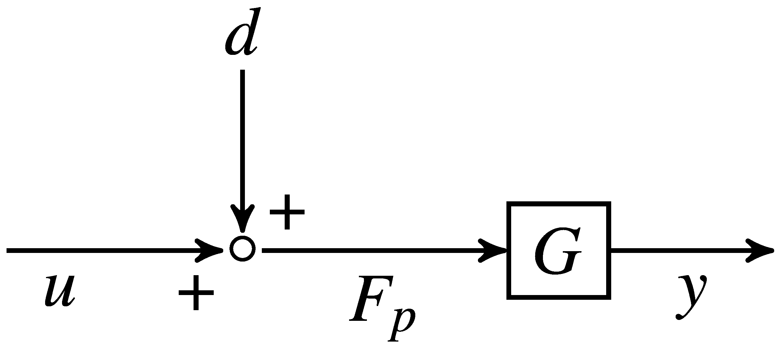
As first formulated by [26], the behavior of a piezoelectric actuator can be described by two subsystems: one is mechanical and the other is electrical. The electrical subsystem is used to describe the system’s reaction to an input voltage u, and the mechanical subsystem is used to describe the relationship between the driving force F p and elongation y p . In these two subsystems, q c is the charge flowing through an equivalent capacitance C; q p is the charge flowing through a transducer T e m ; H ( q ) is the source of hysteresis with a charge flow q = q c + q p ; K p and Γ p are stiffness and damping constants, respectively; and M p is the mass of the actuator (Figure 1 [27]). The equivalent block structure of a piezo-actuated stage per the definition of these two subsystems is shown in Figure 2 [27]; G denotes the linear motion of the stage. The linear transfer function satisfies the relation G = C ( s I A ) B , where s is the Laplace operator, and the matrices A, B, and C constitute the state-space realization
x ˙ = A x + B F p y = C x ,
where x R n is an unknown state variable.
In this study’s proposed scheme, undesired hysteresis is treated as an unknown external disturbance, and the block diagram in Figure 2 can be transformed such that it has the structure illustrated in Figure 3, where d ( t ) = ( T e m 1 ) u T e m H ( q ) , q = ( T e m K p 1 + C T e m 1 ) F p .

2.2. Upper Bound of Disturbance

Because nonlinear hysteresis is treated as an unknown disturbance, a complex model of hysteresis is not required. The only piece of information required for hysteresis control is the upper bound of the disturbance. The classical Prandtl-Ishlinskii (P-I) model [9] is employed to model this upper bound. This model is only used to analyze the structure of the unknown disturbance. The P-I model is constructed on the basis of a one-side operator F o [ v ] ( t ) with a threshold h for a piecewise monotonic input function v ( t ) [9]. As illustrated in Figure 4, the operator is defined as:
w ( 0 ) = F o [ v ] ( 0 ) = f o ( v ( 0 ) , 0 ) w ( t ) = F o [ v ] ( t ) = f o ( v ( t ) , w ( t i ) )
for t [ t i , t i + 1 ] , 0 i N 1 , and
f o ( v , w ) = max ( v h , min ( v , w ) ) .
The time index i is such that the function v ( t ) is monotonic in the interval t [ t i , t i + 1 ] , where t i = 0 for all i. According to the operator (2), the relationship between the input v and output y P I of the P-I model is defined as follows [9]:
y P I ( t ) = P [ v ] ( t ) = p 0 v ( t ) + 0 H p ( h ) F o [ v ] ( t ) d h ,
where p 0 is a constant, p ( h ) is a density function, and H is the maximum value of the threshold h. For the system structure in Figure 2, the hysteresis model is hidden in the relation between the control input u and driving force F p . For this input–output pair, the P-I model becomes:
F p ( t ) = P [ u ] ( t ) = p 0 u ( t ) + 0 H p ( h ) F o [ u ] ( t ) d h .
If the aforementioned model is applied to the system structure in Figure 3, the disturbance is
d ( t ) = ( p 0 1 ) u ( t ) + 0 H p ( h ) F o [ u ] ( t ) d h ,
and the relation
F p = u + d
holds as a result. According to Figure 4, the upper bound of w ( t ) is
| w ( t ) | k 1 | v ( t ) | + k 0
for some positive constants k 1 and k 0 ; therefore, the upper bound of the disturbance (6) is derived as
| d ( t ) | c 1 | u ( t ) | + c 0
for some positive constants c 1 and c 0 . Note that the disturbance here is input dependent, and the system structure is then represented in a disturbance rejection problem after modeling.

3. Control Design and Stability Analysis

In this study, the hysteresis compensation problem is transformed into a disturbance rejection problem for an input-dependent disturbance, and the objective is to suppress the unknown external disturbance while preserving tracking performance. The control structure for suppressing this unknown external disturbance is based on sliding-mode control because it is robust to unknown disturbances and system uncertainties; this control structure can be designed even if (1) the system transfer function and state information are unknown and (2) the unknown disturbance is input dependent. The design of the control structure rests on some basic system-related Assumptions.
Assumption 1.
The system transfer function G ( s ) in Figure 3 is minimum phase.
Assumption 2.
The system transfer function has a relative degree r.
Assumption 3.
The desired reference signal y r is assumed to be sufficiently smooth: there exists a known constant k 0 such that y r ( r ) k for all i = 0 , r .
According to the definition of relative degree [29], Assumption 2 guarantees that C A i B = 0 for i < r 1 and C A r 1 B 0 .
The input–output relation of the control system (1) satisfies the state transformation [29]
x = T η z , T R n × n ,
in which the first set of system states z R r is called an external state comprising the consecutive output derivatives
z = y y ˙ y ( r 1 ) = C x C A x C A r 1 x
and the second set of states η describes the internal state or zero dynamic, where the stability is dominated by the position of the open-loop zeros of the relevant system. The ideal sliding variable is given as
σ = e ( r 1 ) + λ r 2 e ( r 2 ) + + λ 1 e ˙ + λ 0 e ,
where e = y y r is the system tracking error, y r is the desired reference signal, and λ i are design coefficients and are chosen such that σ = 0 is a stable ordinary differential equation of e for the existence of the sliding mode. According to the definition of an external state (11) and Assumption 3, a lumped disturbance containing all λ i coefficients and the derivatives of e is defined as:
Δ p = C A r x y r ( r ) + C A r 1 B d + λ r 2 e ( r 1 ) + + λ 1 e ¨ + λ 0 e ˙
and the upper bound of the disturbance is verified:
Δ p c 4 x + c 3 | u | + c 2
for some positive constants c 4 , c 2 and c 3 < 1 . Note that the sliding variable (12) comprises the derivatives of the tracking error e, which cannot be directly known in real-world applications. Thus, a differentiator is required for the estimation of the derivatives.
Drawing on [21,23], this study adopted the LTR observer [23] as a differentiator to estimate the required error derivatives. The LTR observer is used as a robust observer to estimate the full system state when the control system is affected by an external state and by input-dependent disturbances [21]. The observer functions well as a differentiator because its Luenburger-type structure can be intuitively applied to a linear system. The error dynamic of the control system in Figure 3 is defined as
E ˙ = A r E + B r ( C A r x + C A r 1 B F p y r ( r ) ) = A r E + B r ( C A r x + C A r 1 B ( u + d ) y r ( r ) )
where
E = e e ˙ e ( r 1 ) = y y ˙ y ( r 1 ) y r y r ˙ y r ( r 1 ) , A r = 0 1 0 0 0 1 0 0 0 , B r = 0 0 1 .
The following LTR observer is used to estimate the error vector E in (15):
E ^ ˙ = A r E ^ + B r C A r 1 B u + L r ( e C r E ^ ) ,
where E ^ = [ e ^ e ^ ˙ e ^ ( r 1 ) ] T is an estimate of the error vector E, L r = Q C r T / μ , C r = [ 1 0 0 ] R r , and Q R r × r is the solution matrix of the observer Riccati equation
Q ( A r + δ I ) T + ( A r + δ I ) Q Q C r T C r Q μ + ξ B r B r T = 0 ,
where μ > 0 , δ > 0 , and ξ > 0 are scalar design parameters. The fact that LTR observer estimation is convergent is expressed in the following theorem.
Theorem 1.
The estimation error of the LTR observer (16) asymptotically approaches a small value E ˜ = E E ^ . Specifically,
lim t E ˜ ϵ 1 x + ϵ 2 | u | + ϵ 3 ,
where l i m ξ ϵ i = 0 for i = 1 , 2 , 3 .
Proof. 
See [21,23] □
With the aid of the LTR observer, the following estimate for the ideal sliding variable (12) is obtained.
σ ^ = e ^ ( r 1 ) + λ r 2 e ^ ( r 2 ) + + λ 1 e ^ ˙ + λ 0 e .
The proposed output-feedback sliding-mode control is
u = ρ 1 σ ^ ρ 2 s g n ( σ ^ ) ,
where ρ 1 > 0 is a scalar design parameter and ρ 2 is a positive constant that satisfies
ρ 2 > c 4 x + c 2 α ( 1 c 3 )
in which α = C A r 1 B and the constants c i ’s are as defined in (9) and (13). The good stability and tracking performance of the proposed control (20) is expressed in the following theorem.
Theorem 2.
The proposed control (20) stabilizes the error dynamic (15), and the system tracking error e converges exponentially to 0 as the design parameter ξ in the observer Riccati Equation (17) approaches infinity.
Proof. 
In this proof, estimation error of sliding variable σ ˜ = σ σ ^ is defined. Choose a Lyapunov candidate V = 1 2 σ 2 , and checking its derivative gives
V ˙ = σ C A r 1 B u + Δ p = σ α ρ 1 σ ^ α ρ 2 s g n ( σ ^ ) + Δ p , α = C A r 1 B .
There might be two possible cases for the square brackets in the last equality.
Case 1: | σ | | σ ˜ | . In this case, according to (12) and (19), σ ˜ = [ 1 , λ r 2 , , λ 1 , λ 0 ] E ˜ , and
| σ | λ ¯ ( ϵ 1 x + ϵ 2 | u | + ϵ 3 ) ,
where λ ¯ = m a x ( λ r 2 λ 0 ) .
Case 2: σ > σ ˜ . In this case, sgn( σ ^ ) = sgn( σ ), Equation (22) becomes
V ˙ α ρ 1 σ 2 + σ α ρ 1 σ ˜ | σ | ( ρ 2 | Δ p | ) < α ρ 1 σ 2 + σ α ρ 1 σ ˜ α ρ 1 | σ | | σ | α ρ 1 σ ˜ α ρ 1 | σ | | σ | α ρ 1 λ ¯ ( ϵ 1 x + ϵ 2 | u | + ϵ 3 ) .
From the last inequality,
| σ | α ρ 1 λ ¯ ( ϵ 1 x + ϵ 2 | u | + ϵ 3 )
after some finite time. Combining (23) and (24),
| σ | α ¯ ( ϵ 1 x + ϵ 2 | u | + ϵ 3 ) ,
where α ¯ = m a x ( λ ¯ , α ρ 1 λ ¯ ) . According to the aforementioned equation, the sliding variable practically converges to zero, with the size of residual set approaching zero as the parameter ξ approaches infinity. The reaching condition of sliding-mode control is therefore fulfilled, and the tracking performance is guaranteed by the design of sliding surface (12). □

4. Experimental Results

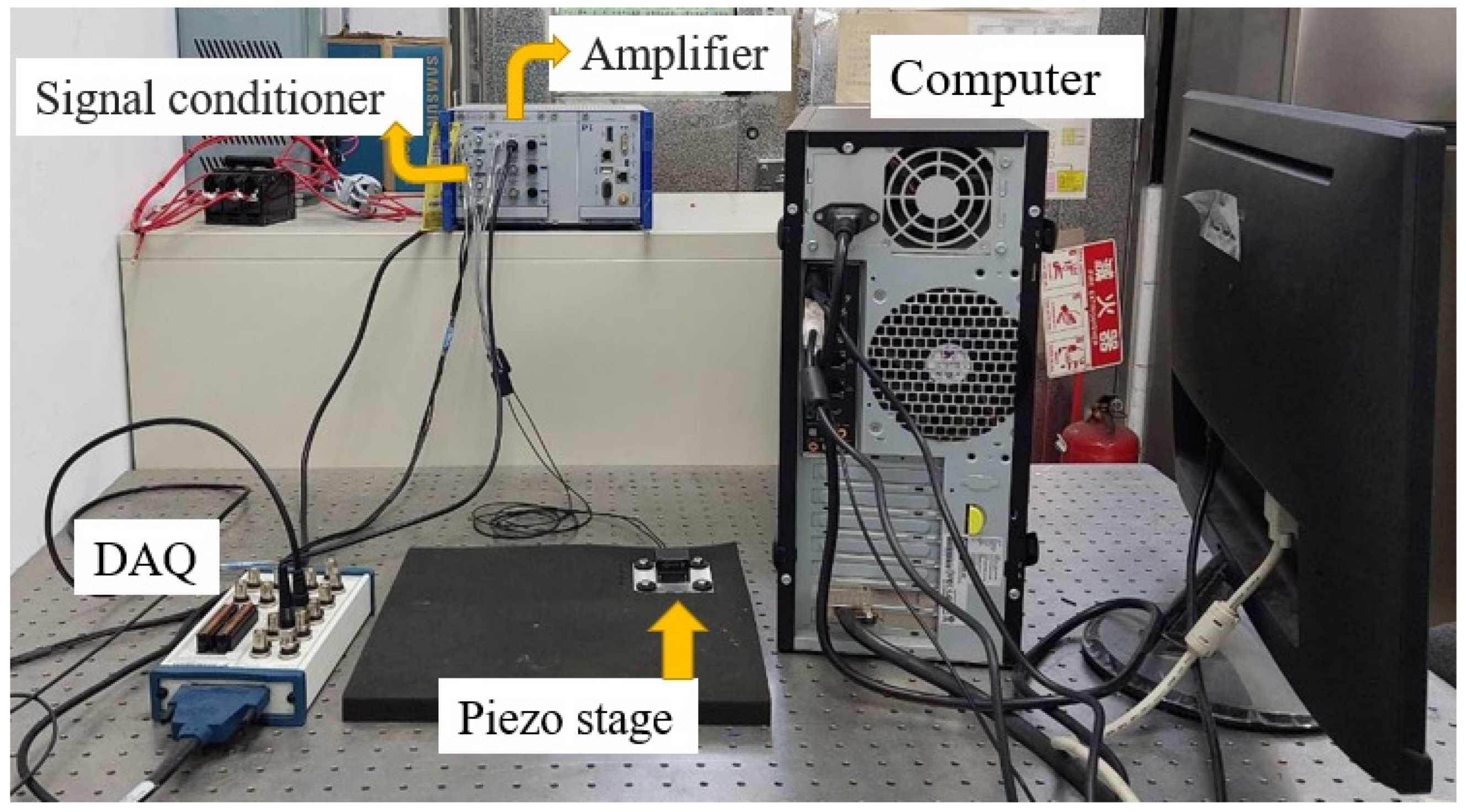
The proposed control algorithm was tested on the x-axis of a piezo-actuated stage PI P-602.2CL (Figure 5). A DAQ card (NI PCI-6346) was employed as an analog–digital interface. The analog I/O channels were arranged using a NI BNC-2110 shielded connector, the input signal was amplified by a PI E-503 amplifier before being fed to the piezoelectric actuators, and the system output displacement was measured using a signal conditioner (PI E-509.C3A). The environment of experimental system is shown in Figure 6. The reference signal was
y r ( t ) = 312.5 + 312.5 sin ( 2 π f t + 1.5 π )
in nano meters. In the design of sliding surface (12), an intuitive approach to verify the derivatives of error signal e is the numerical difference method
e k ( i ) e k ( i 1 ) e k 1 ( i 1 ) T ,
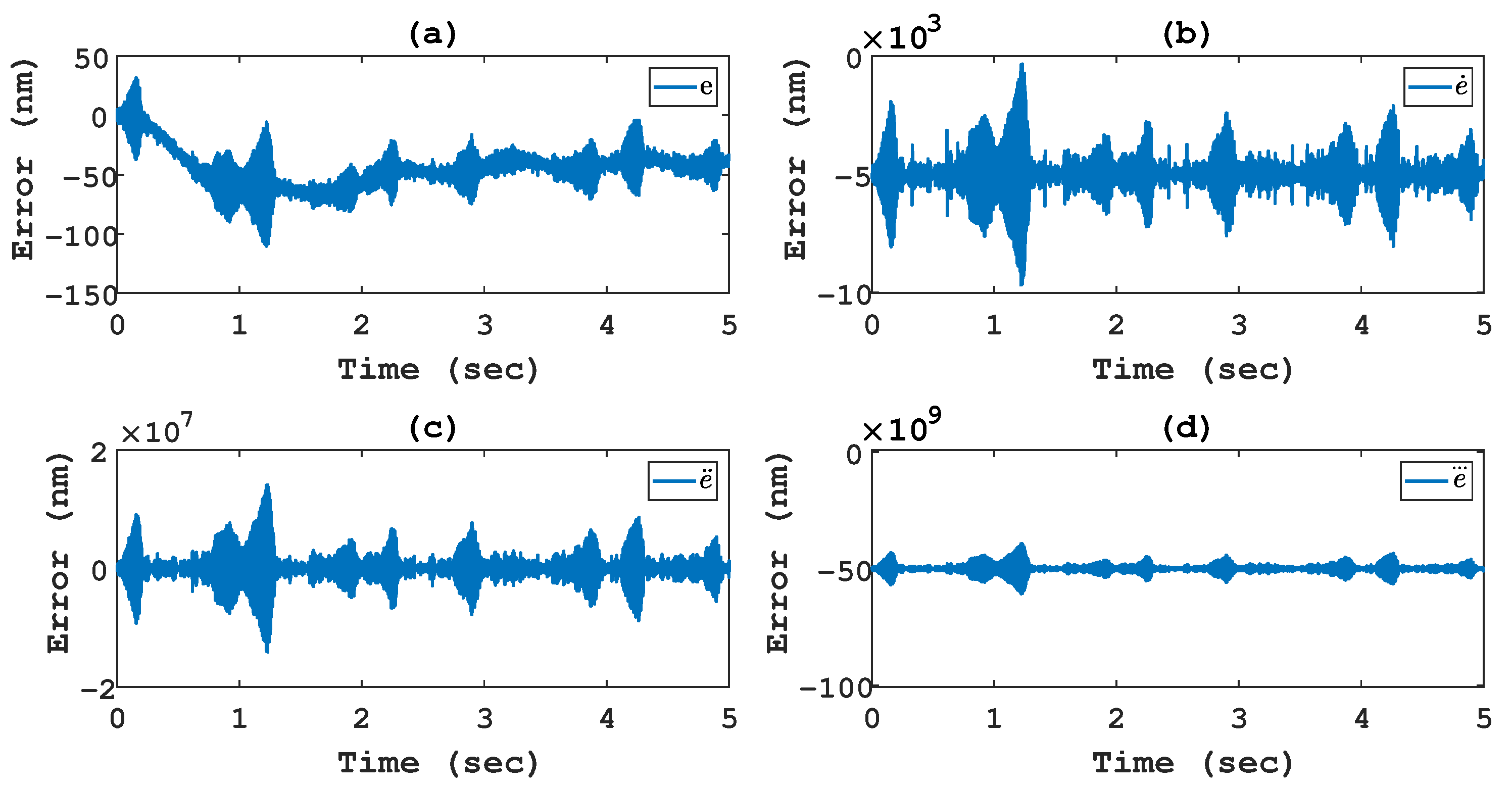
where e ( i ) denotes the i’th order derivative of error signal e, the subscript k is the discrete-time index, and T is the sampling period of control system. However, the conventional numerical difference approach (26) failed to provide the approximation when the error signal is corrupted by the measurement noise. As shown is Figure 7, even if the noisy signal in sub figure (a) is filtered by a third-order low-pass filter
F ( s ) = q s + q 3 , q = 20 π ,
before the numerical difference approach (26) is applied, the behavior of measurement noise still dominate the approximations and overwhelm the quantity of error signal. By contrast, the LTR observer (16) is employed as a robust differentiator to estimate the derivatives of error signal, with the design parameters δ = μ = 1 and ξ = 10 7 in the Riccati Equation (17). As shown in Figure 8, the LTR observer (16) estimates the derivatives more accurately even if the error signal is corrupted by measurement noise, which confirmed the robustness of LTR observer to measurement noise, and demonstrated the effectiveness of the proposed control scheme.
With the aid of the LTR observer, the control design (20) is therefore realizable, and the coefficients for the sliding variable (19) were r = 4 , λ 2 = 12 , λ 1 = 48 , and λ 0 = 64 . The coefficients λ 0 , λ 1 and λ 2 define the convergent speed when the state trajectory hits the sliding surface σ = 0 , and r theoretically denotes the relative degree of the system as in Assumption 2. In this research, the relative degree r was found as the minimum value that the control design (20) experimentally stabilizes the system.
To eliminate undesirable high-frequency chattering in the sliding mode control design (20), the control law (20) was replaced by a continuous boundary layer function [30]
u = ρ 1 σ ^ ρ 2 σ ^ σ ^ + ϵ
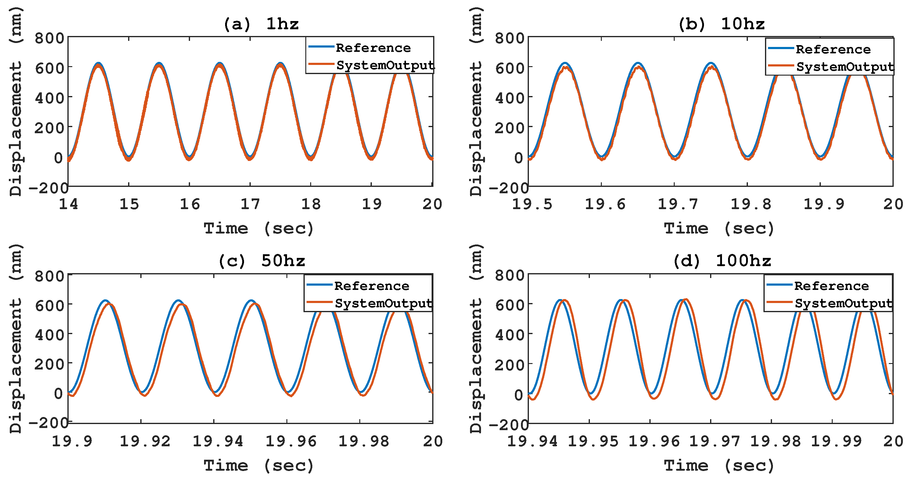
with ρ 1 = 0 , ρ 2 = 0.7 and ϵ = 10 . The experimental results are presented in Figure 9 with the input frequency f = 1 , 10 , 50 , 100 (Hz) in (25), and the tracking errors are listed in Table 1, in which e r m e is the root-mean-square error and e p e r c e n t = e r m s / 625 . It is seen the proposed control structure completed the tracking mission even if the error signal is corrupted by the measurement noise, and the tracking errors increase with the input frequency since the hysteresis loop grows with the input frequency [31].
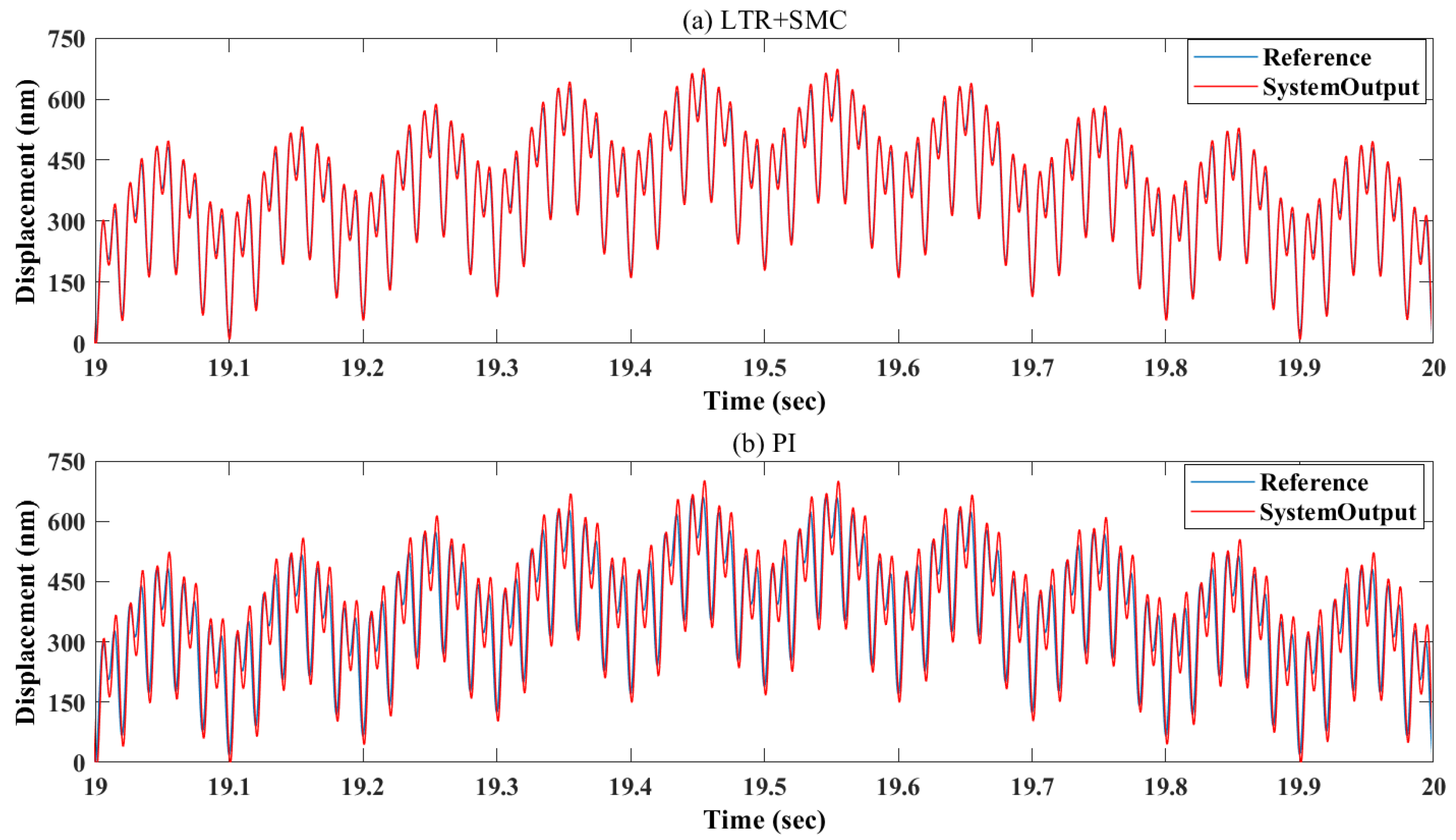
To verity the capability of the proposed control design, a reference signal with multiple frequencies
y m ( t ) = 312.5 + 312.5 sin ( 2 π t + 1.5 π ) + sin ( 20 π t + 1.5 π ) + sin ( 100 π t + 1.5 π ) + sin ( 200 π t + 1.5 π )
was applied to the experimental environment, and a standard PI control with K P = 2.7 and K I = 0.42 was tested as a comparison. The control gains K P and K I were chosen that the PI controller minimizes the tracking error. In Figure 10, it is seen the proposed control design demonstrates a superior performance, and Table 2 shows that the proposed control design performs only 65.79 % of root-mean-square error of the PI controller in steady state.

5. Conclusions

This study proposes an output-feedback sliding-mode control for piezo-actuated stages when state measurements and a system transfer function are unavailable. In this study’s scheme, nonlinear hysteresis is considered an unknown input-dependent disturbance, and a robust LTR observer is used to estimate the differentiation required for disturbance rejection control. The stability of the proposed observer-based control design is rigorously analyzed. In experiments, the results show the LTR observer successively estimate the derivatives of a noisy error signal, whereas the conventional numerical approach fails to approximate, and the proposed control design is capable to track a reference trajectory with multiple frequencies.

Author Contributions

Conceptualization, Y.-L.Y.; data curation, Y.-L.Y., H.-W.P., and Y.-H.S.; formal analysis, Y.-L.Y.; funding acquisition, Y.-L.Y.; investigation, Y.-L.Y., H.-W.P., and Y.-H.S.; methodology, Y.-L.Y., and H.-W.P.; project administration, Y.-L.Y.; resources, Y.-L.Y.; software, H.-W.P. and Y.-H.S.; supervision, Y.-L.Y.; validation, Y.-L.Y.; visualization, Y.-L.Y., H.-W.P., and Y.-H.S.; writing-original draft, Y.-L.Y. and H.-W.P.; writing-review and editing, Y.-L.Y. All authors have read and agreed to the published version of the manuscript.

Funding

This research was funded by the National Science and Technology Council of Taiwan under Grant Number MOST 108-2218-E-027-011-.

Institutional Review Board Statement

Not applicable.

Informed Consent Statement

Not applicable.

Data Availability Statement

Not applicable.

Conflicts of Interest

The authors declare no conflict of interest.

References

  1. Tang, H.; Li, Y. A New Flexure-Based Y-θ Nanomanipulator With Nanometer-Scale Resolution and Millimeter-Scale Workspace. IEEE/ASME Trans. Mechatron. 2014, 20, 1320–1330. [Google Scholar] [CrossRef]
  2. Ghosh, B.; Jain, R.; Majumder, S.; Roy, S.; Mukhopadhyay, S. Experimental performance evaluation of smart bimorph piezoelectric actuator and its application in micro robotics. Microsyst. Technol. 2017, 23, 4619–4635. [Google Scholar] [CrossRef]
  3. Salapaka, S.M.; Salapaka, M.V. Scanning probe microscopy. IEEE Control Syst. Mag. 2008, 28, 65–83. [Google Scholar]
  4. Sabarianand, D.; Karthikeyan, P.; Muthuramalingam, T. A review on control strategies for compensation of hysteresis and creep on piezoelectric actuators based micro systems. Mech. Syst. Signal Process. 2020, 140, 106634. [Google Scholar] [CrossRef]
  5. Li, Y.; Xu, Q. A totally decoupled piezo-driven XYZ flexure parallel micropositioning stage for micro/nanomanipulation. IEEE Trans. Autom. Sci. Eng. 2010, 8, 265–279. [Google Scholar] [CrossRef]
  6. Zhu, H.; Pang, C.K.; Teo, T.J. A flexure-based parallel actuation dual-stage system for large-stroke nanopositioning. IEEE Trans. Ind. Electron. 2017, 64, 5553–5563. [Google Scholar] [CrossRef]
  7. Feng, Z.; Ling, J.; Ming, M.; Liang, W.; Tan, K.K.; Xiao, X. Signal-transformation-based repetitive control of spiral trajectory for piezoelectric nanopositioning stages. IEEE/ASME Trans. Mechatron. 2020, 25, 1634–1645. [Google Scholar] [CrossRef]
  8. Gu, G.Y.; Zhu, L.M.; Su, C.Y.; Ding, H.; Fatikow, S. Modeling and control of piezo-actuated nanopositioning stages: A survey. IEEE Trans. Autom. Sci. Eng. 2014, 13, 313–332. [Google Scholar] [CrossRef]
  9. Brokate, M.; Sprekels, J. Hysteresis and Phase Transitions; Springer Science & Business Media: Berlin/Heidelberg, Germany, 1996; Volume 121. [Google Scholar]
  10. Preisach, F. Über die magnetische Nachwirkung. Z. Phys. 1935, 94, 277–302. [Google Scholar] [CrossRef]
  11. Krasnosel’skii, M.A.; Pokrovskii, A.V. Systems with Hysteresis; Springer Science & Business Media: Berlin/Heidelberg, Germany, 2012. [Google Scholar]
  12. Mayergoyz, I. Mathematical models of hysteresis. IEEE Trans. Magn. 1986, 22, 603–608. [Google Scholar] [CrossRef] [Green Version]
  13. Wen, Y.K. Method for random vibration of hysteretic systems. J. Eng. Mech. Div. 1976, 102, 249–263. [Google Scholar] [CrossRef]
  14. Kodera, N.; Sakashita, M.; Ando, T. Dynamic proportional-integral-differential controller for high-speed atomic force microscopy. Rev. Sci. Instrum. 2006, 77, 083704. [Google Scholar] [CrossRef] [Green Version]
  15. Tang, H.; Li, Y. Development and active disturbance rejection control of a compliant micro-/nanopositioning piezostage with dual mode. IEEE Trans. Ind. Electron. 2013, 61, 1475–1492. [Google Scholar] [CrossRef]
  16. Merry, R.J.; Holierhoek, J.L.; Van De Molengraft, M.J.; Steinbuch, M. Gain scheduling control of a walking piezo actuator. IEEE/ASME Trans. Mechatron. 2013, 19, 954–962. [Google Scholar] [CrossRef]
  17. Zhong, J.; Yao, B. Adaptive robust precision motion control of a piezoelectric positioning stage. IEEE Trans. Control Syst. Technol. 2008, 16, 1039–1046. [Google Scholar] [CrossRef]
  18. Abidi, K.; Sabanovic, A. Sliding-mode control for high-precision motion of a piezostage. IEEE Trans. Ind. Electron. 2007, 54, 629–637. [Google Scholar] [CrossRef] [Green Version]
  19. Xu, J.X.; Abidi, K. Discrete-time output integral sliding-mode control for a piezomotor-driven linear motion stage. IEEE Trans. Ind. Electron. 2008, 55, 3917–3926. [Google Scholar]
  20. Shen, J.C.; Jywe, W.Y.; Liu, C.H.; Jian, Y.T.; Yang, J. Sliding-mode control of a three-degrees-of-freedom nanopositioner. Asian J. Control 2008, 10, 267–276. [Google Scholar] [CrossRef]
  21. Yeh, Y.L. Output Feedback Tracking Sliding Mode Control for Systems with State-and Input-Dependent Disturbances. Actuators 2021, 10, 117. [Google Scholar] [CrossRef]
  22. Utkin, V.; Guldner, J.; Shi, J. Sliding Mode Control in Electro-Mechanical Systems; CRC Press: Boca Raton, FL, USA, 2017. [Google Scholar]
  23. Chen, M.S.; Chen, C.H.; Yang, F.Y. An LTR-observer-based dynamic sliding mode control for chattering reduction. Automatica 2007, 43, 1111–1116. [Google Scholar] [CrossRef]
  24. Levant, A. Higher-order sliding modes, differentiation and output-feedback control. Int. J. Control 2003, 76, 924–941. [Google Scholar] [CrossRef]
  25. Oliveira, T.R.; Estrada, A.; Fridman, L.M. Global and exact HOSM differentiator with dynamic gains for output-feedback sliding mode control. Automatica 2017, 81, 156–163. [Google Scholar] [CrossRef]
  26. Goldfarb, M.; Celanovic, N. Modeling piezoelectric stack actuators for control of micromanipulation. IEEE Control Syst. Mag. 1997, 17, 69–79. [Google Scholar]
  27. Yeh, Y.L.; Yen, J.Y.; Wu, C.J. Adaptation-Enhanced Model-Based Control with Charge Feedback for Piezo-Actuated Stage. Asian J. Control 2020, 22, 104–116. [Google Scholar] [CrossRef]
  28. Gu, G.Y.; Zhu, L.M.; Su, C.Y. Modeling and compensation of asymmetric hysteresis nonlinearity for piezoceramic actuators with a modified Prandtl–Ishlinskii model. IEEE Trans. Ind. Electron. 2013, 61, 1583–1595. [Google Scholar] [CrossRef]
  29. Marquez, H.J. Nonlinear Control Systems: Analysis and Design; John Wiley: Hoboken, NJ, USA, 2003; Volume 161. [Google Scholar]
  30. Burton, J.; Zinober, A.S. Continuous approximation of variable structure control. Int. J. Syst. Sci. 1986, 17, 875–885. [Google Scholar] [CrossRef]
  31. Xiao, S.; Li, Y. Modeling and high dynamic compensating the rate-dependent hysteresis of piezoelectric actuators via a novel modified inverse Preisach model. IEEE Trans. Control Syst. Technol. 2012, 21, 1549–1557. [Google Scholar] [CrossRef]
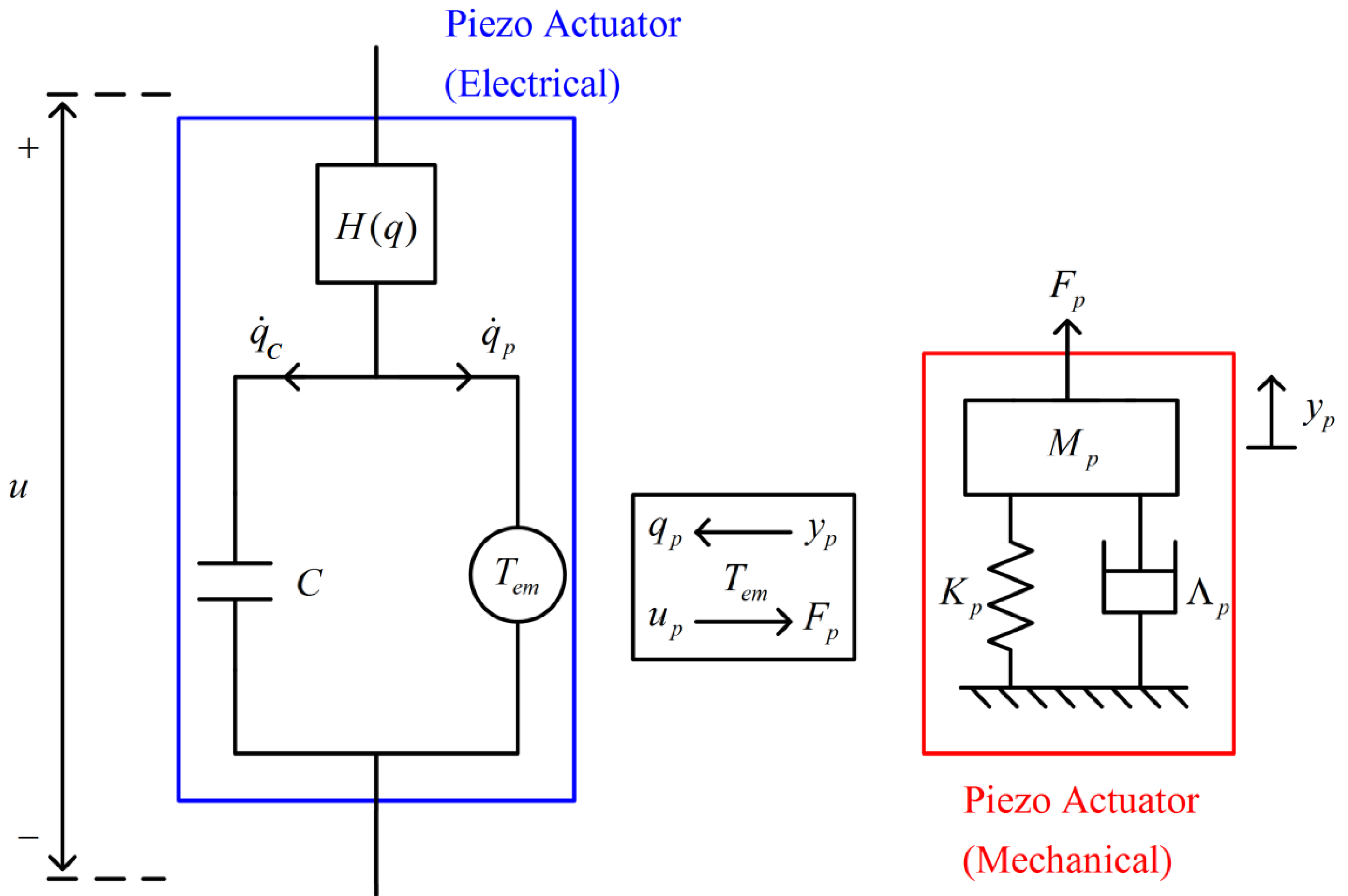
Figure 1. Subsystems of a piezoelectric actuator [27].
Machines 11 00152 g001
Figure 2. Block diagram of a piezoelectric actuator.
Machines 11 00152 g002
Figure 3. Equivalent block structure of the piezo-actuated stage.
Machines 11 00152 g003
Figure 4. Input-output relationships of the OSP operator [28].
Machines 11 00152 g004
Figure 5. Experimental setup.
Machines 11 00152 g005
Figure 6. Environment of experimental system.
Machines 11 00152 g006
Figure 7. Temporal evolution of low-pass filter with: (a) an error signal e, (b) the first-order derivative e ˙ , (c) the second-order derivative e ¨ , (d) the third-order derivative e at 1 Hz.
Machines 11 00152 g007
Figure 8. Temporal evolution of LTR observer with (a) an error signal e, (b) the estimation of the first-order derivative e ^ ˙ , (c) the estimation of the second-order derivative e ^ ¨ , (d) the estimation of the third-order derivative e ^ at 1 Hz.
Machines 11 00152 g008
Figure 9. Output trajectories of proposed control scheme when (a) f = 1 (Hz), (b) f = 10 (Hz), (c) f = 50 (Hz), (d) f = 100 (Hz).
Machines 11 00152 g009
Figure 10. Output trajectories of (a) proposed control scheme and (b) PI control with multiple input frequencies.
Machines 11 00152 g010
Table 1. Controller performance results.
f (Hz) e rms (nm) e percent (%)
114.72.36
1025.74.11
5056.89.09
10092.814.84
Table 2. Controller performance results with multiple frequencies.
Controller e rms (nm) e percent (%)
LTR+SMC97.816.5
PI149.324.7
Disclaimer/Publisher’s Note: The statements, opinions and data contained in all publications are solely those of the individual author(s) and contributor(s) and not of MDPI and/or the editor(s). MDPI and/or the editor(s) disclaim responsibility for any injury to people or property resulting from any ideas, methods, instructions or products referred to in the content.