The Disk-Halo Distinction of Galaxies Using Faraday Tomography

Department of Astrophysics/IMAPP, Radboud University Nijmegen, P.O. Box 9010, NL-6500 GL Nijmegen, The Netherlands
Galaxies 2019, 7(1), 1; https://doi.org/10.3390/galaxies7010001
Submission received: 28 November 2018
/
Revised: 13 December 2018
/
Accepted: 17 December 2018
/
Published: 21 December 2018
(This article belongs to the Special Issue The Power of Faraday Tomography)
Abstract
:Faraday tomography allows us to study the distribution and properties of the magnetoionic medium of galaxies through the Faraday effect. However, this can be achieved only after the Faraday spectrum is interpreted. One approach is using galactic ISM/magnetism models to investigate how characteristic properties of the galaxies in the physical depth space are reflected to the Faraday spectrum. In this paper, I employ a realistic Galactic ISM/magnetism model and calculate the intrinsic Faraday spectrum of face-on galaxies, especially focusing on the galactic disk-halo structure and on the presence of the coherent, vertical magnetic field. I also calculate the Faraday depth cubes of the Milky Way from the model. I discuss the possibility of studying the disk and halo structures by means of Faraday tomography.
1. Introduction
Faraday tomography aims to determine the distribution and properties of magnetoionic medium along the line of sight (LOS) toward, and within, astronomical objects through the Faraday effect. This technique requires wide-band low frequency (≲10 GHz) polarization data, and thus the Square Kilometre Array and its precursors/pathfinders make it possible to use the technique for studying cosmic magnetism. Cosmic magnetism studies using Faraday tomography require the interpretation of the Faraday spectrum, , which gives the intensity of synchrotron polarization as a function of the Faraday depth, . is obtained from the observed polarization spectrum, , through the equation
where the is the wavelength (see e.g., [1,2]). The Faraday depth is expressed as
where is the thermal electron number density, is the LOS component of the magnetic field, is the integration variable in physical distance, and r is an arbitrary physical distance. One of the difficulties in using the technique, as implied by Equation (2), is that can change its sign along the LOS due to turbulence and it causes the lack of a one-to-one relation between the Faraday depth and the physical depth.
There have been many challenges to apply Faraday tomography for studying objects with various scales including the external galaxies and the Milky Way. For studying the diffuse emission on the sky, Faraday depth cubes are often used, which consist of two-dimensional images as a function of the Faraday depth, . Previous studies have found interesting emission features on large scales, which are associated with the Milky Way, from Faraday depth cubes (e.g., [3,4,5]). However, the interpretation of the physical depth information from the is necessary to fully extract the potential of Faraday tomography. For the purpose of localizing the emissions, previous studies have made various attempts: they simply assumed the uniform Faraday rotating medium as the Galactic halo (or thick-disk) (e.g., [4]), used optical photometric data showing a morphological correspondence (e.g., [5]), or used the information of H line which is a good tracer of warm ionized gas (e.g., [3,6]).
Another complementary approach to interpret the properties of can be to use simulation results. In simulations, we have the information of the magnetic field as a function of physical depth and also we can calculate the Faraday spectrum. Once we can know how the galactic properties in the physical depth are reflected in the Faraday depth, it can provide how to extract the information in the physical depth from the Faraday spectrum. The earlier works using simple models found that the magnetic field reversals along the LOS causes singularities in (Faraday caustics) and that a turbulent magnetic field basically appears as many small-scale components on (Faraday forests) [7,8,9]. In Ideguchi et al. [10], they studied of a small portion of the external face-on galaxies using the realistic Galactic model constructed by Akahori et al. [11]. They found that the realistic of galaxies is complicated, but some global galactic properties can affect the shape of . For instance, the presence of coherent, vertical magnetic field and the larger scale height of thermal electron density result in a wider width of . As emphasized by Ideguchi et al. [10], the study using the realistic Galactic model provides the realistic of galaxies, but therefore, it is not straightforward to interpret the results due to its complexity. Following the studies by Ideguchi et al. [10], Ideguchi et al. [12] employ “simple, toy models” for the magnetic field in order for the deeper understanding of the behavior of . They found that the shape of will converge to a well defined average by observing multiple LOSs covering a region of ≳(10 coherent length of turbulence). They also showed that with these average , the shape-characterizing parameters such as width, skewness, and kurtosis also converge to consistent values, and the information of the coherent, vertical magnetic field can be extracted.
In this paper, I demonstrate some additional analysis using the Galactic model by Akahori et al. [11]. I calculate the in the same manner as Ideguchi et al. [10]. First, I focus on the effect of the Galactic disk and halo (or thick-disk) structures on , which is motivated from the expectation in Ideguchi et al. [10] that the near-side halo along the LOS constructs the peak at . In addition, I study the presence of coherent, vertical magnetic field by separately looking at each contributions from the disk and halos on . Then, I try to compare the realistic with the study in Ideguchi et al. [12]. Since Ideguchi et al. [12] considered the only disk to make the situation as simple as possible, I calculate the realistic by considering only the contribution from disk. Interpretation of of external galaxies is useful not only to study magnetic fields associated with the galaxies themselves, but also could be useful to probe intergalactic magnetic field embedded between two galaxies as a gap between two components in space (e.g., [13,14]). Though the previous works focused on one-dimensional , I also construct Faraday depth cubes of the Milky Way using the Galactic model. I study how the presence of the vertical magnetic field and the halo affect the polarization structures in the Faraday depth cubes. Study of of the Milky Way is important to understand our galaxy, and also the information of diffuse emissions from the Galactic interstellar medium is essential for studying the outside of our galaxy including the epoch of reionization. Below, I briefly explain the Galactic model in Section 2. Then, I show the results in Section 3 and the summary and discussion follows in Section 4.
2. Galactic Model
In this paper, I employ a Galactic model constructed by Akahori et al. [11] (see also [10]). Note that any model can be used for this study as long as it contains information of 3-D magnetic field vector and thermal and cosmic-ray electron densities. This model consists of the global, regular component as well as the turbulent, random component. The regular component is modeled using the thermal electron density model of Cordes and Lazio [15] and magnetic field models including an axisymmetric spiral field and a halo toroidal field [16] as well as a dipole poloidal field that produces a coherent vertical field near the Earth [17]. The random component is modeled by MHD turbulence simulations [18]. They set the integral scale of turbulence as pc. The computational region of the model is kpc centered on the location of the Earth, kpc, where the plane coincides with the galactic midplane with y pointing the anti-galactic center and z penetrating the midplane. This is a model of the solar neighborhood and I study the Faraday spectrum of the Milky Way by using it, but I also use it as an external galaxy. I regard the z direction as the line of sight (LOS), and this is equivalent to considering the Milky Way towards high galactic latitude or the external face-on galaxies. The region is divided by 32 pixels in x and y and by 1280 pixels in z.
For the calculation of , I consider two cases: and G, where is the strength of coherent magnetic fields that vertically penetrates the disk. The coherent magnetic field is written as [17]
where . For G case, is set so that G around kpc, while it is absent for case. Figure 1 shows examples of the LOS distributions (through z direction) of physical quantities for the case of (a) and of G (b). The top and the second top panels are the thermal electron density, , in cm and the parallel component of the magnetic field along the LOS, , in G, respectively. The third panels from the top show the Faraday depth, , in rad m, which are calculated from and using Equation (2). Note that since these are the cases where the model is treated as an external galaxy, by design. For the “” case, since the is random with the mean of 0, the changes randomly with respect to the LOS. On the other hand, for the “G” case, is a monotonic function of the physical depth since the is random but always positive along z-axis (and thus it points away from us). The bottom panels show the distributions of polarization intensity, , whose peaks are normalized to 1. One can see both the emissions from the disk at |z| ≲ 1 kpc and that from the halo at |z| ≳ 1 kpc. I consider the region of |z| ≲ 1 kpc as the disk and |z| ≳ 1 kpc as the halos for the following calculations.
3. Results
3.1. Faraday Spectrum of External Galaxies
Figure 2 shows the Faraday spectra, , calculated from the Galactic model, which are integrated over the all LOSs through the galaxy (i.e., 32 × 32 LOSs). Here, the model is considered as an external face-on galaxy, and emission and Faraday rotation due to medium intervening in between the galaxy and the observer are not assumed. The left panels are the results of the “” case (a), and the right panels are the results of the “G” case (b). Each eight panels show the different realizations of turbulence. Note that I show a in the top middle panel of the “” case, which was the representative one shown in Figure 4 in Ideguchi et al. [10]. The overall shapes of in each panel varies substantially for different configurations of turbulence as reported by Ideguchi et al. [10]. In the case, some have a single peak and others have multiple peaks, some are broad and others are thin. If there is non-zero mean , clearly show the broader feature compared with the non- case. This can be expected since the is always positive (points away from us) and thus can reach the large negative value. Also, in both cases, they are not smooth and contain many small-scale components. They are attributed to the turbulence of the magnetic field and/or the thermal electron density along the line of sight (LOS).
Next, I examine the in a bit more detail. The in each panel is categorized into three in different colors: the contributions from the halo which is located at the near side along the LOS (magenta), the disk (cyan) and the far-side halo (green). In the case of , it is apparent that the sharp component around is always the contribution from the near-side halo. This is because, since no emitting and Faraday rotating medium is assumed between the observer and the galaxy, the first, nearest computational cells along the LOS do not experience any Faraday rotation and thus they have . By going deeper along the LOS through the near-side halo, there is polarized emission that is Faraday rotated due to the magnetic field associated with the halo itself, while cannot be very large since the region affecting is relatively short. As a result, the emission from the near-side halo, though it is not bright compared with the disk, is accumulated within a narrow width in space and hence the near-side halo creates a sharp component in at . Going further into the disk, there are larger P, and , resulting in the emission experiencing a larger amount of Faraday rotation than the halo and can reach larger . Hence, the emission from the disk can have bright and broad features in . At last, the emission from the far-side halo is, unlike the near-side one, experience different amount of Faraday rotation at different LOSs (Faraday dispersion) due to the disk and the near-side halo and thus it is distributed widely in the space.
The results of the “G” case is also interpretable with the same concept as the “” case mentioned above. At first, the sharp component around is constructed by the near-side halo by the same reason described above. One difference from the “” case is that, because there is the mean positive , the mean of emissions are negative. Thus, the emission from farther physical depth is preferentially distributed at larger . This results in the whose distribution in Faraday depth space principally corresponds to that in physical depth since the distribution is the monotonic function of the physical depth as explained in Section 2. This feature always appears for every realizations of turbulence shown in Figure 2. This feature may allow us to probe the disk-halo structures of face-on galaxies by means of Faraday tomography.
3.2. The Shape of Faraday Spectrum of External Galaxies
As implied in the previous subsection, the global properties of galaxies (especially, this is the coherent, vertical magnetic field in this paper) can affect the shape of . As with the previous works [10,12], I use the width (standard deviation), skewness and kurtosis of as shape-characterizing parameters to quantify the shape of . Here, I try to calculate the parameters only from the disk for the purpose to compare them with the simple galactic models. Thus, I only use the computational region of to avoid any contribution of the halos including the Faraday rotation and its dispersion due to the near-side halo. Figure 3 shows the scattered plots and the one-dimensional probability distribution of the parameters, constructed from eight hundred realizations of turbulence. Note that the 1-D distribution of the whole region (red) is the same as those in Figures 8–10 in Ideguchi et al. [10]. Apparently, the results from two cases are almost unchanged for both “” and “G” cases, except the width for the “G” case. This exception occurs simply because the emissions from halos, which are distributed on the both sides of the disk in space, are excluded for the “only disk” case and that leads to its smaller width compared with the “whole region” case.
Though the effects of the halo on the moments of is small, the tendency of the difference between the “” and “G” cases are consistent with the results of Ideguchi et al. [12]. That is, for the “G” case, the width gets slightly larger, the skewness is shifted to non-zero (negative in this case) and the extent of scatter of it is smaller, and the kurtosis gets slightly smaller and the extent of scatter of it is smaller, compared with the “” case.
3.3. Faraday Depth Cubes of the Milky Way
Figure 4 shows the absolute polarization intensity () images calculated from the Galactic model. Here, the model is considered as the Milky Way towards high galactic latitude. Thus, only the half of the computational region, , is used to calculate . Note that all LOSs start from different locations in the midplane for simplicity, which is different from real observations where all LOSs originate at the same coordinate. I will discuss about how this may affect the results in Section 4. Also, I try to calculate with and without a halo to study the contribution of it to of the Milky Way. There are two groups of panels: the left is the results from the “” case (a) and the right is that from the “G” case (b). In each group, the left column shows the results of the “with halo” case and the right is the “without halo” case. The top panels show the map which is integrated along the LOS from to 10 kpc for the “with halo” case and to 1 kpc for the “without halo” case. Polarized emissions are integrated as complex values, so this integral accounts for differences in polarization angle along the LOS. The panels from the second top show the maps at different , i.e., the slice maps from the Faraday depth cubes. Polarized emissions are also integrated as complex values, but in this case, emissions within resolutions are integrated. The resolutions in are 2 rad m for the “” case and 6 rad m for the “G” case. Note that the polarization intensities are normalized since this paper only concentrates on the morphology of polarization emissions: the peak value within a map is normalized to 1 in the case of the top panels and the peak value in the Faraday depth cubes are normalized to 1 for other maps.
At first, one can see from the “” and “with halo” case (the most left column in the Figure 4) that there is a broad emission in the upper region at rad m which seems to move to lower region through rad m with showing the characteristic morphologies. By comparing the “with halo” and “without halo” cases, one can see the contribution of the halo to the Faraday depth cube. In the “” case, it can be seen that the halo emissions exist in various . Especially, the characteristic features appear at rad m, where the halo emissions look to be superposed on results of the “without halo” case. This is expected from the results in Figure 2 since the of the “” case shows that the emissions from the far-side halo are dispersed in space due to the Faraday-rotating medium which exists between the (far-side) halo and the observer.
In the case of “G”, the morphologies at rad m look similar between “with halo” and “without halo” cases. On the other hand, at larger from rad m, the emissions from the halo are superposed on the results of the “without halo” case. It is rather interesting that at much larger from rad m, there are some emission for the “with halo” case while the emission is hardly seen for the “without halo” case. This may imply the possibility to study the disk-halo structures of the Milky Way separately by means of Faraday tomography.
4. Summary and Discussion
In this paper, following Ideguchi et al. [10], I tried the further analysis of the realistic Faraday spectrum of galaxies using the realistic Galactic model constructed by Akahori et al. [11]. First, I assumed observations of external face-on galaxies with two cases: and G, where is the mean strength of coherent, vertical magnetic fields. I separated contributions of the disk and halos structures to the shape of and looked at how a resultant, realistic is constructed. It was shown that the near-halo causes a sharp structure at for the both cases. In both cases, the disk and far-halo are broadly distributed in space. In the case this is caused by the turbulent and , while for G case the non-zero produces a monotonic relationship between physical depth and . This relationship produces a distinction of halo-disk-halo structures even in .
In Ideguchi et al. [12], they showed that the shape of becomes smooth by observing the region which covers ≥(10 coherent length of turbulence) by using a simple toy model. Then, they mentioned that, in Ideguchi et al. [10], the covering region of (500 pc) with pc that provides ∼44 LOSs is not enough for to be converged to a well defined average. In this work, I suspect the structures of halos as a cause of complexity of the realistic , since the simple model assumes only a disk while the realistic model contains both disk and halos. To check this, I calculated realistic only from the disk structure () for 800 realizations of turbulence, and investigated them using moments of . It became clear that distributions of the moments are barely changed between the case with and without the halos. Also, distributions of the moments of the realistic seemed to be more scattered than the case using the simple model with 44 LOSs. These results imply that the complexity of realistic also comes from the non-uniform distributions of physical quantities (e.g., exponential distribution for cosmic-ray electron density). Though the study using the simple toy model by Ideguchi et al. [12] assume uniform distributions of physical quantities, for deeper understanding of the realistic , it is necessary to study the simple model by adding realistic assumptions one by one.
Finally, I calculated the Faraday depth cubes of the Milky Way by using a half of the calculation region (i.e., ) of the Galactic model. Specifically, I tried to study contributions of the halo to Faraday depth cubes. An interesting result is that for the case of “G”, morphologies of the emission at large are produced by the emission from the halo. Hence, if there is non-zero in the Milky Way, it may be possible to separate emissions of the halo from that of the disk and to study them separately by means of Faraday tomography. The same goes for external face-on galaxies if there is non-zero and we may be able to study the halo-disk-halo structures. Indeed, it is observationally found that there is a non-zero vertical magnetic field toward the south Galactic pole (e.g., [19,20]). This may enable us to make detailed studies of the magnetic field of the disk and halo in the Milky Way by Faraday tomography.
While this paper employed the realistic Galactic ISM/magnetism, several simple assumptions were still made. Let me briefly mention the effects of these simple assumptions. In this work, all LOSs are assumed to start from different locations in the midplane for simplicity, while in real observations, nearer parts of the LOS are closer together. This affects to less emissions in the nearer parts, and thus emissions from the disk is expected to get small. On the other hand, the result that a halo emission appears at large in the G case is barely affected by this assumption. In addition, this work adopted a model where the sign of is constant everywhere, which arises from the fact that coherent component of magnetic fields is stronger than random component. This may not be true in the case where is non-zero, but is still weaker than the random component. When strengths of coherent and random components of magnetic fields are comparable, it is expected that emissions at large mainly comes from halo but also partly from disk, which makes it more difficult to separate disk and halo contributions in . In a case where random component is much stronger than coherent component, the result is thought to be essentially no different from the case, and thus it is basically impossible to distinguish halo and disk structures in . Finally, I discuss an effect of inclination of galaxies. Although this paper only studied face-on galaxies, if a galactic disc is inclined, part of large scale magnetic fields which is parallel to the disc can be a LOS component. This could make complicated, but may also make it possible to address magnetic fields parallel to discs from the shape of . This study will be reported in a forthcoming paper (Eguchi et al. in preparation).
This study investigated the “intrinsic” Faraday spectrum of external galaxies and the Milky Way. However, it is impossible to fully reconstruct the intrinsic Faraday spectrum in practice. This is because of our limited frequency coverage, and the appearance of observational artifacts in data processing (e.g., instrumental polarization). Especially, the reconstruction of the Faraday spectrum highly depends on the observation frequency and its coverage. Some of important parameters introduced in Brentjens and de Bruyn [2] explain that while frequency coverage at lower frequencies provides higher precision in space, lower frequency observations also provide less sensitivity to broad structure in space. For instance, the High Band Antenna of the Low Frequency Array [21] (120–240 MHz) has ∼1 rad m resolution and is sensitive for the scale up to ∼1 rad m in space, while the full band of the Australian Square Kilometre Array Pathfinder [22] (700–1800 MHz) has the ∼22 rad m resolution and is sensitive for the scale up to ∼113 rad m. As shown in the results of this paper, the Faraday spectrum of galaxies tend to be diffuse in space with the widths of larger than 10 rad m as well as the small-scale components due to turbulence. For the reconstruction of such , it is necessary to use wide-band polarization data from low frequency (∼100 MHz) to higher frequency (a few GHz). The necessary frequency coverage and appropriate Faraday tomography methods for reconstructing such complicated Faraday spectrum will be investigated in the forthcoming studies.
Funding
This research received no external funding.
Acknowledgments
I thank the referees for their constructive comments on the manuscript.
Conflicts of Interest
The author declares no conflict of interest.
References
- Burn, B.J. On the depolarization of discrete radio sources by Faraday dispersion. Mon. Not. R. Astron. Soc. 1966, 133, 67. [Google Scholar] [CrossRef]
- Brentjens, M.A.; de Bruyn, A.G. Faraday rotation measure synthesis. Astron. Astrophys. 2005, 441, 1217–1228. [Google Scholar] [Green Version]
- Jelić, V.; de Bruyn, A.G.; Pandey, V.N.; Mevius, M.; Haverkorn, M.; Brentjens, M.A.; Koopmans, L.V.E.; Zaroubi, S.; Abdalla, F.B.; Asad, K.M.B.; et al. Linear polarization structures in LOFAR observations of the interstellar medium in the 3C 196 field. Astron. Astrophys. 2015, 583, A137. [Google Scholar]
- Lenc, E.; Gaensler, B.M.; Sun, X.H.; Sadler, E.M.; Willis, A.G.; Barry, N.; Beardsley, A.P.; Bell, M.E.; Bernardi, G.; Bowman, J.D.; et al. Low-frequency Observations of Linearly Polarized Structures in the Interstellar Medium near the South Galactic Pole. Astrophys. J. 2016, 830, 38. [Google Scholar] [CrossRef]
- Van Eck, C.L.; Haverkorn, M.; Alves, M.I.R.; Beck, R.; de Bruyn, A.G.; Enßlin, T.; Farnes, J.S.; Ferrière, K.; Heald, G.; Horellou, C.; et al. Faraday tomography of the local interstellar medium with LOFAR: Galactic foregrounds towards IC 342. Astron. Astrophys. 2017, 597, A98. [Google Scholar] [Green Version]
- Brentjens, M.A. Wide field polarimetry around the Perseus cluster at 350 MHz. Astron. Astrophys. 2011, 526, A9. [Google Scholar]
- Bell, M.R.; Junklewitz, H.; Enßlin, T.A. Faraday caustics. Singularities in the Faraday spectrum and their utility as probes of magnetic field properties. Astron. Astrophys. 2011, 535, A85. [Google Scholar]
- Frick, P.; Sokoloff, D.; Stepanov, R.; Beck, R. Faraday rotation measure synthesis for magnetic fields of galaxies. Mon. Not. R. Astron. Soc. 2011, 414, 2540–2549. [Google Scholar] [CrossRef] [Green Version]
- Beck, R.; Frick, P.; Stepanov, R.; Sokoloff, D. Recognizing magnetic structures by present and future radio telescopes with Faraday rotation measure synthesis. Astron. Astrophys. 2012, 543, A113. [Google Scholar] [Green Version]
- Ideguchi, S.; Tashiro, Y.; Akahori, T.; Takahashi, K.; Ryu, D. Faraday Dispersion Functions of Galaxies. Astrophys. J. 2014, 792, 51. [Google Scholar] [CrossRef]
- Akahori, T.; Ryu, D.; Kim, J.; Gaensler, B.M. Simulated Faraday Rotation Measures toward High Galactic Latitudes. Astrophys. J. 2013, 767, 150. [Google Scholar] [CrossRef]
- Ideguchi, S.; Tashiro, Y.; Akahori, T.; Takahashi, K.; Ryu, D. Study of the Vertical Magnetic Field in Face-on Galaxies Using Faraday Tomography. Astrophys. J. 2017, 843, 146. [Google Scholar] [CrossRef] [Green Version]
- Akahori, T.; Kumazaki, K.; Takahashi, K.; Ryu, D. Exploring the intergalactic magnetic field by means of Faraday tomography. Publ. Astron. Soc. Jpn. 2014, 66, 65. [Google Scholar] [CrossRef]
- Ideguchi, S.; Takahashi, K.; Akahori, T.; Kumazaki, K.; Ryu, D. Fisher analysis on wide-band polarimetry for probing the intergalactic magnetic field. Publ. Astron. Soc. Jpn. 2014, 66, 5. [Google Scholar] [CrossRef]
- Cordes, J.M.; Lazio, T.J.W. NE2001.I. A New Model for the Galactic Distribution of Free Electrons and its Fluctuations. arXiv, 2002; arXiv:astro-ph/0207156. [Google Scholar]
- Sun, X.H.; Reich, W.; Waelkens, A.; Enßlin, T.A. Radio observational constraints on Galactic 3D-emission models. Astron. Astrophys. 2008, 477, 573–592. [Google Scholar]
- Giacinti, G.; Kachelrieß, M.; Semikoz, D.V.; Sigl, G. Ultrahigh energy nuclei in the galactic magnetic field. J. Cosmol. Astro-Part. Phys. 2010, 2010, 036. [Google Scholar] [CrossRef]
- Kim, J.; Ryu, D.; Jones, T.W.; Hong, S.S. A Multidimensional Code for Isothermal Magnetohydrodynamic Flows in Astrophysics. Astrophys. J. 1999, 514, 506–519. [Google Scholar] [CrossRef] [Green Version]
- Taylor, A.R.; Stil, J.M.; Sunstrum, C. A Rotation Measure Image of the Sky. Astrophys. J. 2009, 702, 1230–1236. [Google Scholar] [CrossRef]
- Mao, S.A.; Gaensler, B.M.; Haverkorn, M.; Zweibel, E.G.; Madsen, G.J.; McClure-Griffiths, N.M.; Shukurov, A.; Kronberg, P.P. A Survey of Extragalactic Faraday Rotation at High Galactic Latitude: The Vertical Magnetic Field of the Milky Way Toward the Galactic Poles. Astrophys. J. 2010, 714, 1170–1186. [Google Scholar] [CrossRef]
- Van Haarlem, M.P.; Wise, M.W.; Gunst, A.W.; Heald, G.; McKean, J.P.; Hessels, J.W.T.; de Bruyn, A.G.; Nijboer, R.; Swinbank, J.; Fallows, R.; et al. LOFAR: The LOw-Frequency ARray. Astron. Astrophys. 2013, 556, A2. [Google Scholar] [Green Version]
- McConnell, D.; Allison, J.R.; Bannister, K.; Bell, M.E.; Bignall, H.E.; Chippendale, A.P.; Edwards, P.G.; Harvey-Smith, L.; Hegarty, S.; Heywood, I.; et al. The Australian Square Kilometre Array Pathfinder: Performance of the Boolardy Engineering Test Array. Publ. Astron. Soc. Aust. 2016, 33, e042. [Google Scholar] [CrossRef]
Figure 1.
(a) LOS (z-axis) distributions for the “” case (left panels) and for the “G” case (right panels). Each panel shows the thermal electron density (), LOS components of the magnetic field (), Faraday depth () calculated from and , and absolute polarized intensity (), from top to bottom. Note that by design, since these are cases where the model is treated as an external galaxy.

Figure 2.
(a) Faraday spectra, , for the “” case (left panels) and for the “G” case (right panels). These are integrated over all LOSs (32 × 32 LOSs). In each case, eight different realizations are shown. Colors in each panel show the contributions from the near-side halo (blue), disk (gray), and far-side halo (red) along the LOS.
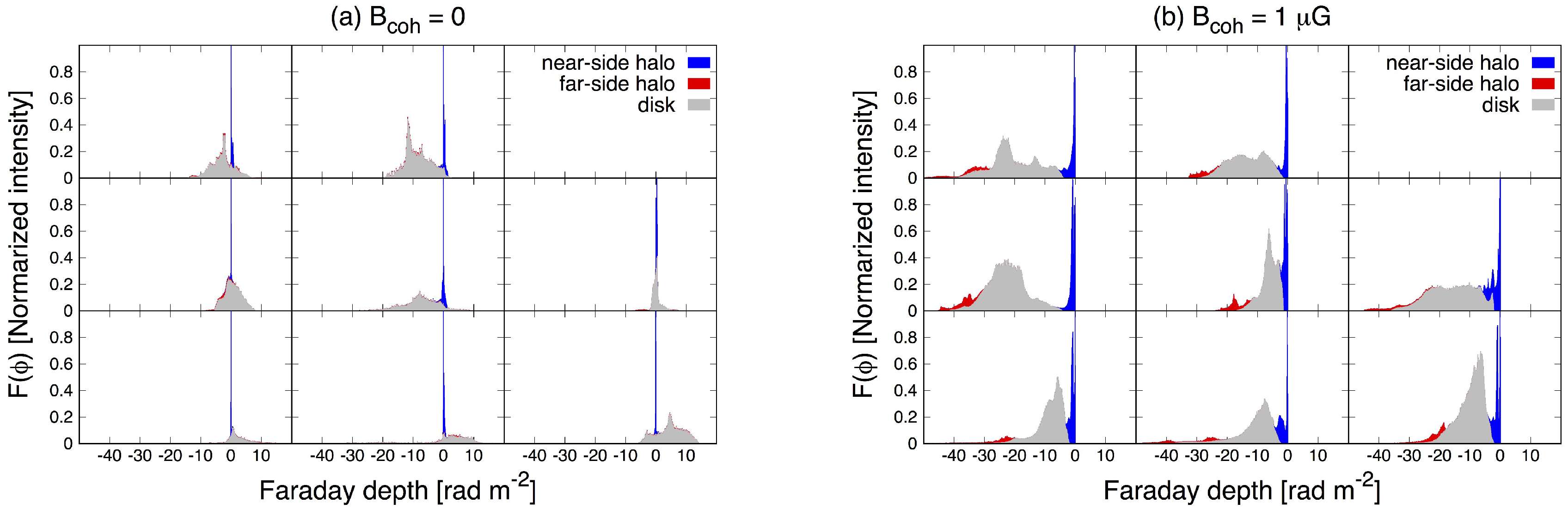
Figure 3.
(a) Scatter plots for shape-characterizing parameters of the Faraday spectrum, , for the “” case (left panels) and for the “G” case (right panels). The calculated from whole region and from only disk shown in red (solid line, plus symbol) and blue (dashed line, cross symbol), respectively. Eight hundred realizations are shown. Top panels of each column are one-dimensional probability distributions of the parameters.

Figure 4.
Normalized, absolute polarization intensity () images. Left two columns show results from the “” case (a) and right two columns show results from the “G” case (b). In each case, the left column shows the “with halo” case and right column shows “without halo” case. Top panels show the LOS-integrated images. Panels from the second top show slice images from the Faraday depth cube at different Faraday depth, . The unit of is in rad m.

© 2018 by the author. Licensee MDPI, Basel, Switzerland. This article is an open access article distributed under the terms and conditions of the Creative Commons Attribution (CC BY) license (http://creativecommons.org/licenses/by/4.0/).
Share and Cite
MDPI and ACS Style
Ideguchi, S. The Disk-Halo Distinction of Galaxies Using Faraday Tomography. Galaxies 2019, 7, 1. https://doi.org/10.3390/galaxies7010001
AMA Style
Ideguchi S. The Disk-Halo Distinction of Galaxies Using Faraday Tomography. Galaxies. 2019; 7(1):1. https://doi.org/10.3390/galaxies7010001
Chicago/Turabian StyleIdeguchi, Shinsuke. 2019. "The Disk-Halo Distinction of Galaxies Using Faraday Tomography" Galaxies 7, no. 1: 1. https://doi.org/10.3390/galaxies7010001
Note that from the first issue of 2016, this journal uses article numbers instead of page numbers. See further details here.