Article

Estimating the Cowper–Symonds Parameters for High-Strength Steel Using DIC Combined with Integral Measures of Deviation

Faculty of Mechanical Engineering, University of Ljubljana, Askerceva 6, 1000 Ljubljana, Slovenia
*
Author to whom correspondence should be addressed.
Metals 2024, 14(9), 992; https://doi.org/10.3390/met14090992 (registering DOI)
Submission received: 19 July 2024 / Revised: 23 August 2024 / Accepted: 27 August 2024 / Published: 31 August 2024

Abstract

:
Cowper–Symonds parameters were estimated for the complex-phase high-strength steel with a commercial name of SZBS800. The parameter estimation was based on a series of conventional tensile tests and unconventional high-strain rate experiments. The parameters were estimated using a reverse engineering approach. LS-Dyna was used for numerical simulations, and the material’s response was modelled using a piece-wise linear plasticity model with a visco-plastic formulation of the Cowper–Symonds material model. A multi-criteria cost function was defined and applied to obtain a response function for the parameters p and C. The cost function was modelled with a response surface, and the optimal parameters were estimated using a real-valued genetic algorithm. The main novelty and innovation of this article is the definition of a cost function that measures a deviation between the deformed geometry of the flat plate-like specimens and the results of the numerical simulations. The results are compared to the relevant literature. A critical evaluation of our results and references is another novelty of this article.

1. Introduction

When modelling high-velocity impact phenomena (e.g., vehicle crashes at high velocities or projectile impacts into load-carrying structures, etc.), material response at high strain rates should be known. One frequently applied practice for considering the high-strain rate effects in the elastic-plastic domain of metals is to adjust the material’s yield stress with the Cowper–Symonds model. In its most common form, the yield stress is modified with the following term [1,2]:
β = 1 + ( ε ˙ p l C ) 1 / p
C and p are the two Cowper–Symonds parameters, ε ˙ p l is plastic strain rate; and β is the yield stress correction factor.
Since high strain rates of ε ˙ p l > 100 are difficult to achieve using universal testing machines, alternative methods were developed for testing specimens of different geometries. Among the most commonly applied testing methods are the Taylor test [3,4,5], split Hopkinson bar test [6,7,8], flywheel test [9,10], and falling weight or drop test [11,12]. In addition, researchers also developed hybrid devices that combine the advantages of the bar-type and different loading type-systems [13,14]. The challenge of using the alternative testing procedures is to estimate the strain-rate dependent material parameters (i.e., the Cowper–Symonds parameters C and p in our case). For this purpose, different optimisation techniques are applied, often combined with a reverse engineering approach. Škrlec et al. [15] showed how the strain-rate-dependent material response of a high-strength steel with the commercial name SZBS800, which was modelled using the Cowper–Symonds model, can be determined using a combination of conventional tensile tests with different strain rates up to 5.4 s−1 and impact ball tests with varying impact velocities that resulted in strain rates up to 450 s−1 (The SZBS800 steel was used in our research because there was no high-strain rate data for this kind of steel in the literature). The impact ball test was a derivation of the impact test that was originally developed for polymer materials [16]. In this approach, the C and p parameters were estimated by minimising a combined cost function that was a superposition of (i) a sum-of-squares deviation between the simulated and measured σ-ε curves emanating from the tensile tests at low-strain rates and (ii) a deviation between the simulated and measured imprint depth and position from impact ball tests at high strain rates. The obtained result for the C and p parameters was compared to the available literature data for comparable high-strength steels:
  • Q390D [17] high-strength steel [18],
  • 2507 [19] super duplex stainless steel [20],
  • S690QL [21] high-strength steel [22,23],
  • 22MnB5 [24] hot-forming high-strength steel [25],
  • HTRB600E [26] high-strength reinforcing steel [27],
  • Multi-phase high yield strength steel (MP800HY), according to [28],
  • B500A [29] commercial high-strength reinforcing steel [30] and
  • HRB500E [31] reinforcing steel bars [32].
A result of this comparison was a conclusion that the estimated values for the C parameter, which are available in the literature, span many orders of magnitude, ranging from 2.68 [20] to 86,700,000 [27]. The range for the p parameter was between 1.31 [18] and 30.4 [15] (with most of the values below 6.7). The highest strain rates, which were achieved during the tests, were between 200 s−1 [22] and 4000 s−1 [25]. By comparing the methodologies and data from the literature, the following possible causes for such differences are listed below:
  • The selected testing method and the achieved strain rates have a significant influence on the estimated parameters. In general, the higher the strain rates achieved, the higher the parameter C.
  • The two parameters C and p are not independent but are strongly correlated.
  • The considered strain-rate range influences the estimated parameters C and p.
  • The forms of the applied Cowper–Symonds model may be different.
  • How the cost function for estimating the strain-rate dependent parameters is defined is important.
Besides the above-mentioned causes, it should be emphasised that different materials have different sensitivity to high-strain rate loads. This is manifested through the Cowper–Symonds parameter p. According to Equation (1), this parameter should always be bigger than one. However, if the parameter p is between 1 and 2, the sensitivity of the material’s yield stress to high strain rates is significant. In contrast, if the parameter p is bigger than 10, the strain-rate sensitivity is small. In the case of the high-strength steel SZBS800, the parameter p was equal to 30.4 [15], which implies that the investigated material is quite insensitive to the strain rate effects. However, this is not uncommon. Other scholars have discovered that some high-strength steel grades are also almost insensitive to strain rate effects, e.g., high-strength armour steels Mars 190, 240, and 300 [33], Weldox 460E steel [34], or high-strength armour steel Protac 500 [35]. Unfortunately, the results from Škrlec et al. [15] cannot be compared to the last three references [33,34,35] because their authors used a Johnson-Cook material model to consider the high-strain rate effects. Since the Johnson-Cook material model is inherently isotropic [1,2] it was decided that it would not be used in our current research. Specifically, the piecewise linear plasticity material model [1,2], which was applied here, enables the consideration of both isotropic and kinematic hardening. In the case of high-strength steel, a presumption of kinematic hardening is more realistic.
According to the challenges listed above, additional effort is needed to obtain better estimates of the Cowper–Symonds parameters C and p for the experimental data of the SZBS800 steel. For this reason, we modified the cost function for estimating the two strain-rate dependent parameters by using an integral measure of deviation between the simulated and experimental results for the shooting ball test. In this manner, a geometric deviation is calculated for the total free surface of the deformed specimen and not only for the point of the maximum indentation depth. To our best knowledge, the presented measure of deviation between the numerical and experimental results (i.e., a cost function) was not applied before for this particular problem. In addition to that, we decided to determine the 3D geometry of the specimen using the contactless optical method. Therefore, the 3D geometry of the deformed specimen is determined using a digital image correlation (DIC) approach that combines pictures made with multiple cameras at different angles, which is a well-known method for obtaining shape information of an object [36,37] or quantifying a specimen response in terms of deformation, strain, and motion during various tests [38,39,40,41]. In addition, the results from the literature [18,20,22,23,25,27,28,30,32] are critically evaluated in this article according to their phenomenological suitability for the Cowper–Symonds material model.
The article is structured as follows: After the introductory section, the material properties of the SZBS800 steel and testing procedures will be briefly presented. Then, a theoretical background on the applied variation of the Cowper–Symonds material model is presented. This specific variation has not been utilised in our previous analyses, and it has the potential to better describe the behaviour of the observed material. The second section ends with a description of the 3D geometry measurements and a definition of the new cost function for estimating the strain-rate dependent parameters. This new cost function is based on measurements of the entire specimen geometry rather than just a few characteristic points, as was performed in our previous research. In the third section, the newly estimated C and p parameters for the SZBS800 steel are shown first. This result is then compared to the Cowper–Symonds data from the literature, which is also critically evaluated and discussed. The article ends with a concluding section, acknowledgements, and a list of references.

2. Materials and Methods

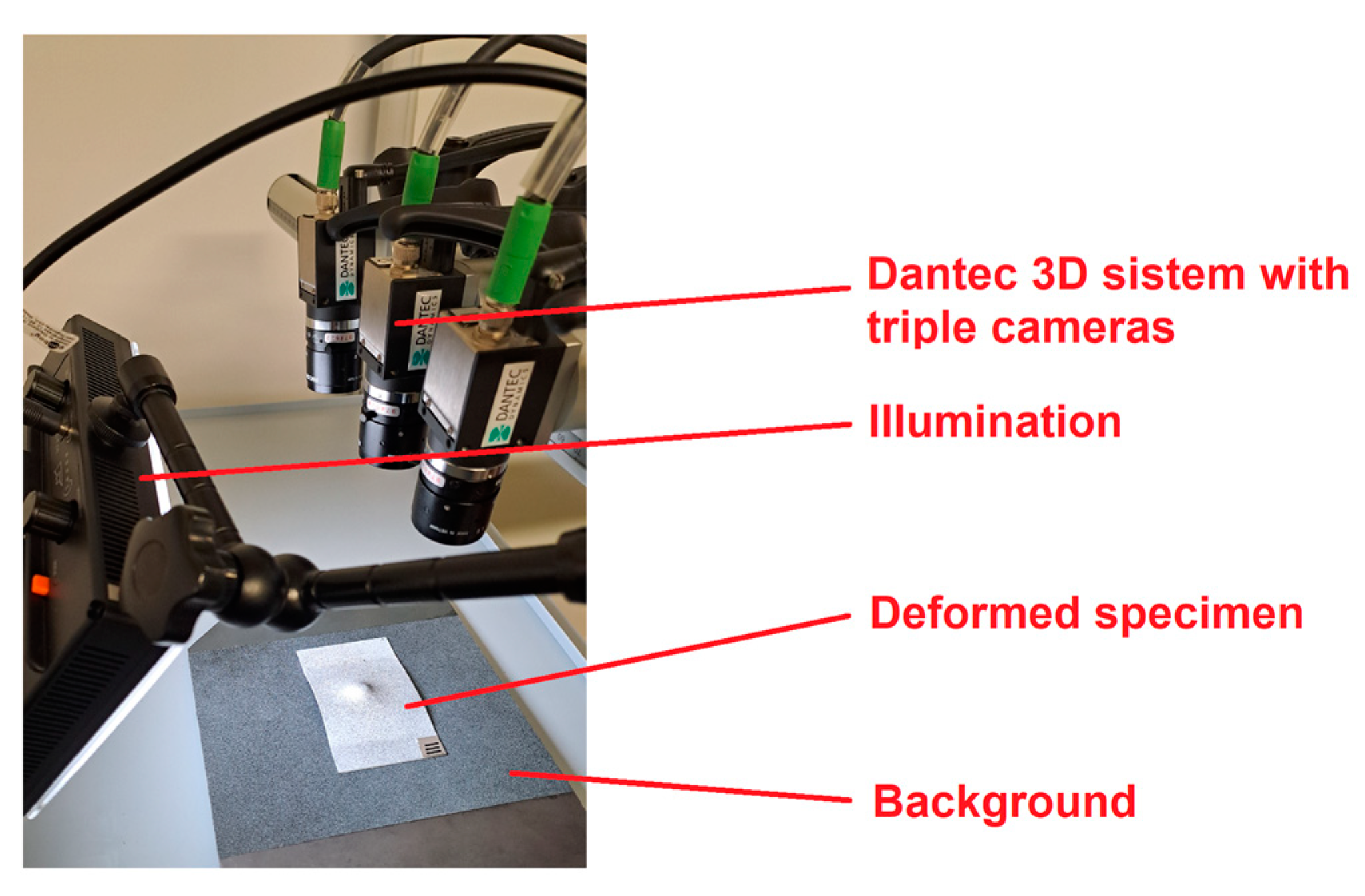
2.1. Experimental Setup

A high-strength steel EN 1.0998 according to [31] (with a commercial name SZBS800 used in continuation of this paper) was the focus of this research. Its chemical composition of the steel is presented in Table 1.
In our previous research [15], low-strain rate and high-strain rate experiments were carried out to characterise the response of this steel. The low strain-rate experiments were performed using a 100 kN servo-hydraulic MTS Landmark 370.10 from MTS Systems Corp., Eden Prairie, MN, USA (MTS testing machine in continuation). The loading rate was selected in such a manner that the strain rates ε ˙ p l between 0.0028   s 1 and 5.4   s 1 were achieved. For this purpose, 1 mm thick dog-bone specimens with a geometry according to the ASTM E8/E8M standard were used [43]; see Figure 1.
At the lowest strain rate, strains were measured with a mechanical extensometer MTS 834.11F-24 from MTS Systems Corp, Eden Prairie, MN, USA (extensometer in continuation), whose gauge length was 25 mm. In addition, a strain distribution was determined using a digital image correlation (DIC) method for each low strain-rate tensile test. During the experiment, the speckled colour pattern on the specimen was recorded with a high-speed camera i-SPEED 508 from IX Cameras, Essex, UK (high-speed camera in continuation). The frame rate was synchronised with the data acquisition sampling rate of the MTS testing machine to 4096 fps. The image resolution was 800 × 1080 pixels. Digital image processing was performed using Istra4D V4.10 software from Dantec Dynamics, Skovlunde, Denmark (Istra4D software in continuation) in order to obtain a load-dependent strain distribution during the tensile test. Altogether, 13 tensile tests were performed.
To achieve strain rates above 100 s−1, a different experimental arrangement was used. This experiment was actually a modified version of a testing arrangement according to the ASTM D5420 standard [16]. A steel ball with a diameter of 13.6 mm and a weight of 10.6 g was shot at high velocity into a rectangular 1 mm thick plate-like specimen with a dimension of 98 × 60 mm2. The specimen was clamped along its two short edges in such a way that it had a free surface of 60 × 60 mm2. The ball used in the experiment was taken from a Schaeffler ball bearing (FAG before) [44]. According to their catalogue, steel balls are made from through-hardened rolling bearing steel 100Cr6 in accordance with [45], with tensile yield strength over 1700 MPa, tensile ultimate strength up to 2300 MPa, and 61 HRC of hardness. The ball was shot to the specimen with a pneumatic gun manufactured for this purpose. The gun outlet and the specimen were positioned in a safety chamber. For the impact tests, two parameters were varied: (i) the impact velocity (between 111 m/s and 155 m/s) and (ii) the impact angle (between 0° and 35°). Each impact experiment was recorded with the high-speed camera. Its recordings were used to improve the accuracy of the measured velocities from the gun’s photosensors. Altogether, nine impact tests were performed. For details, see Škrlec et al. [15]. In contrast to the low strain-rate tensile tests, it was difficult to determine the strain rate during the impact tests. With the help of the numerical simulations, which are explained later, it was estimated that the strain rate during the impact tests was between 300 s−1 and 450 s−1.
The geometry of the deformed specimens after the impact ball test was measured using a digital image correlation (DIC) method. A random pattern with acrylic paint (white base colour with black dots) was first applied to each of the deformed specimens. Additionally, another random colour pattern with a black base and white dots was applied to a flat plate, to which the specimens were placed during the photography stage; see Figure 2. The use of two different random colour patterns provided slightly higher contrast in the images, allowing us to distinguish between the specimen and the base. A coordinate system was later defined with fixed points on the base, ensuring that all the processed images were acquired with the exact same specimen position. The multiple images of the painted, deformed specimens were made with a 3D FlexDIC system from Dantec Dynamics, Skovlunde, Denmark (3D DIC system in continuation). The specimens were illuminated with an LED lighting module. Three cameras were positioned very close to the object in order to maximise the use of the sensor’s full resolution. This arrangement enhanced the image quality and subsequently improved the accuracy of the calculated coordinate values in the Istra4D software.
For image correlation, it is necessary to perform a 3D calibration of the system position (i.e., cameras and focal lengths) before capturing the images. Each specimen was photographed with an image acquisition frequency of 10 Hz, and 10 images were saved. The captured images were processed using the Istra4D software. Correlation of the images enables reconstruction of the subject’s contour. The density of the calculation points for the image correlation was chosen so that the contours of the deformed specimens were reliably detected. In this manner, the complete deformed geometry of the specimen was captured as a cloud of points arranged in a grid-like formation. These data sets (i.e., one data set per deformed specimen) formed a basis for the reverse engineering method, in which the same experiment was simulated to obtain deformed specimen geometries for different combinations of the Cowper–Symonds material parameters.

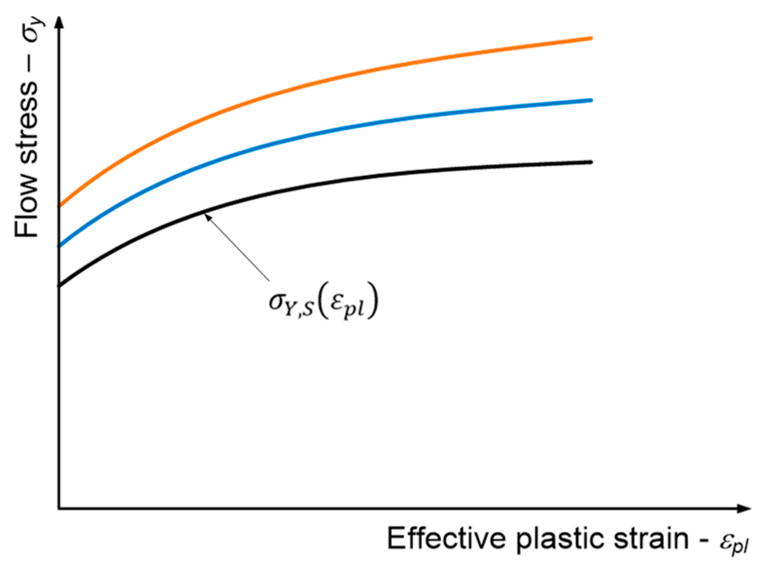
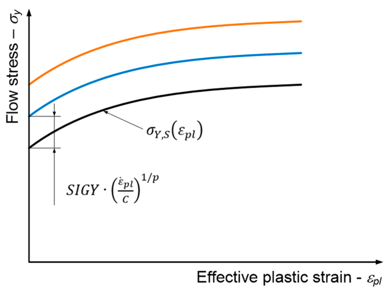
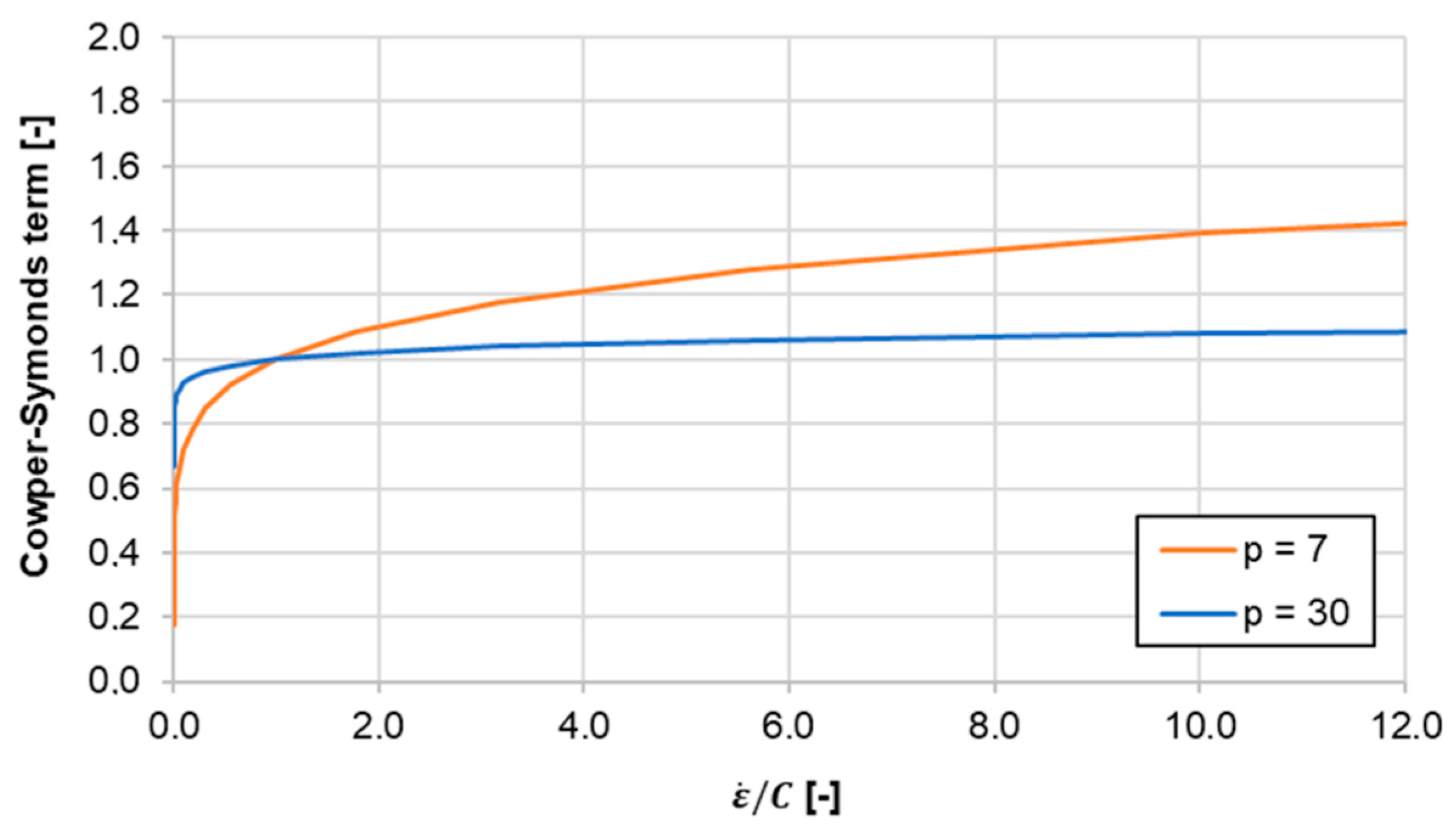
2.2. Modelling the Strain-Rate-Dependent Material Response

All the numerical simulations were performed with explicit finite element method software LS-Dyna V971 R11.1, LSTC, Livermore, CA, USA. The material model MAT_PIECEWISE_LINEAR_PLASTICITY (Ls-Dyna MAT_24) was used to model the response of the SZBS800 steel. In essence, this is a Besseling material model [46] with the addition of the strain-rate dependent term. According to the LS-Dyna documentation [1,2], there are two possible formulations for considering strain rate effects. The conventional approach, as presented in Equation (2), scales the quasi-static flow curve according to the Cowper–Symonds model; see also Figure 3:
σ Y ( ε p l ) = σ Y , S ( ε p l ) · [ 1 + ( ε ˙ p l C ) 1 / p ]
This means that the plastic flow curves are not parallel to each other but are diverging towards the right-hand side of the σ Y - ε p l diagram at higher strain rates (see Figure 2), which is not the case for most steels. For steel, the flow curves are usually only shifted along the stress axis according to the strain rate. The same happened in our case, as can be seen from the true stress-true strain diagram in Section 3.1.
To obtain a translation of the plastic flow curve along the flow-stress axis, an alternative formulation (i.e., the visco-plastic) of the strain-rate dependency needs to be applied; see also Figure 4:
σ Y ( ε p l ) = σ Y , S ( ε p l ) + S I G Y · ( ε ˙ p l C ) 1 / p
In this case, a parallel vertical translation is determined using the term S I G Y · ( ε ˙ p l / C ) 1 / p . Due to a well-expressed parallelism of the tensile curves at different strain rates in our case, we opted for the second formulation, which includes the active visco-plastic option. According to the LS-Dyna MAT_24 material model [1,2], a value of σ Y , S ( ε p l = 0 ) should define an initial yield stress value at pure static loading (i.e., at strain rate ε ˙ p l = 0 ). Since the SIGY parameter acts only as a scale factor for the yield stress in combination with the Cowper–Symonds term, its value depends directly on the value of the strain rate that is selected for the quasi-static loading. In our case, the strain rate for the quasi-static load was set to a value of 10−10 s−1. The flow curve σ Y , S ( ε p l ) in the MAT_24 material model was modelled with a piece-wise linear function starting below the knee—point-of the measured true-stress–true strain curve. Consequently, as can also be seen in Figure 4, it can be concluded that the SIGY parameter has nothing to do with real yield stress but is merely a material parameter that is applied to adjust a vertical shift of the flow curve as a function of the strain rate. Moreover, we discovered in our previous research [15] that Equation (3) models the material response very poorly if the SIGY parameter is set to the value of the yield stress for the smallest measured strain rate.

2.3. Estimating the Material Parameters from the Experimental Data

The three parameters SIGY, C, and p in Equation (3) are estimated with a two-stage procedure:
  • Phase 1: a rough estimation of the three parameters that is based on the low strain-rate tensile tests.
  • Phase 2: fine-tuning of the C and p parameters using multi-criterion cost function combined with numerical optimisation and reverse engineering. In this phase, low-strain rate and high-strain rate experiments are considered.
After a very rough estimate of the usable domains for the three parameters SIGY, C, and p, in which the SIGY parameter space was divided into five increments (i.e., 200, 300, 400, 500, and 600 MPa), the improved estimates of the three parameters were obtained using the grid search method in Phase 1. For each combination of the parameters, the flow-stress curves were calculated analytically with Equation (3) for the strain rates that were achieved during the low strain-rate tensile tests. These analytical flow-stress curves σ ^ Y ( ε p l ) were compared to the experimentally determined flow-stress curves σ Y ( ε p l ) using a sum of squared distances cost function SSQDLSR,i for each combination k of the three parameters SIGY, C, and p:
S S Q D L S R , k = L S R _ c a s e s [ ε _ d o m a i n ( σ Y ( ε p l ) σ ^ Y , k ( ε p l ) ) 2 ]
The quasi-static flow σ Y , S ( ε p l ) curve was used, as presented in Figure 5. The division of the C and p spaces for this optimisation step is presented in Table 2. In Phase 1, the best estimates for the three parameters were as follows: SIGY = 400 MPa, C = 210 s−1 and p = 30. Further details on Phase 1 can be found in Škrlec et al. [15].
As already mentioned in the introductory section, the main drawback of our previous research [15] is linked to the formulation of the multi-criterion cost function, which was applied in Phase 2. For this reason, a new cost function was defined to compare the results of numerical simulations to the deformed shapes of the plate-like specimens from the shooting ball test. The main idea is to find a combination of the three parameters SIGY, C, and p that best suits the response of the dog-bone specimens from the tensile test as well as plate-like specimens from the impact ball test. By using Equation (4), the material model is compared to the low strain rate experiments, which have been explained for Phase 1. Now, as we describe the methodology for Phase 2, attention is turned to the high-strain-rate experiments. Since the C and p parameters cannot be estimated directly from these experiments, the reverse engineering approach is applied. By following this approach, explicit dynamic finite-element simulations of the shooting ball test were carried out for the selected combinations of the parameters SIGY, C, and p. The deformed specimen geometry from the simulations was compared to the measured geometry of the tested specimens. The procedure is described in the continuation of this section.
For the explicit dynamic finite-element (FE) simulations, LS-Dyna software was used. The FE model consisted of the plate-like specimen and the flying ball right before the impact. The ball was modelled with 19,208 eight-node constant-stress solid finite elements and a rigid material (MAT_20) to shorten the simulation times. During this research, a pilot series of simulations were carried out in which Besseling’s plastic-kinematic hardening material model (MAT_3) was used for the ball instead of the rigid material model. The material data for the ball was taken from the producer’s user manual [44]. It turned out that the difference in deformations between the elastic-plastic and rigid ball material was less than 0.1%. However, the simulation time for the elastic-plastic ball material was three times longer.
An initial velocity vector was prescribed to the ball to mimic the ball’s velocity and impact angle during the shooting test. The steel-sheet model had 9984 four-node shell finite elements with a Hughes-Liu co-rotational formulation. For the plate, the previously described LS-Dyna MAT_24 material model with a Von Mises plasticity, a kinematic hardening rule and a viscous formulation of the Cowper–Symonds model was applied. For the material parameters, the same static flow curve σ Y , S ( ε p l ) (see Figure 5) and SIGY parameter (SIGY = 400 MPa) were used as in Phase 1. The division of the C and p spaces for Phase 2 is presented in Table 2. Between the steel sheet and the rigid ball, there was a surface-to-surface contact with a penalty formulation and a friction coefficient μ = 0.2. The FE model was fixed at the same spot as the real specimen during the impact test. A typical final geometry from the shooting ball simulations is presented in Figure 6. More details on these simulations can be found in Škrlec et al. [15].
The simulation results obtained with LS-Dyna were stored in binout files and further processed using the Python programming language. Post-processing of binout files was conducted with a qd Python package 0.8.9. For each simulation, the nodal (x, y, z) coordinates were read. The coordinates before impact and after the impact are depicted in Figure 7.
To summarise the simulation results for different boundary conditions (i.e., impact velocity and impact angle) and different material parameters (C and p), a reference image was constructed in the following manner: Let Y be nx × nx matrix, which represents the reference image. The nx and ny are the number of rows and columns, respectively. Let i 1 , , n x and j 1 , , n y be the matrix entry indices. Each matrix entry i, j contains the value of displacement y i , j at the corresponding coordinate values xi and zi. The coordinates xi and zi are calculated as follows:
x i = x m i n + i · d x
z j = z m i n   + j · d z
The values xmin and zmin give the coordinate origin values of respective coordinates and are dependent on coordinate placement while performing a simulation. The respective coordinate increment dx and dz can be calculated as:
d x = x m a x x m i n n x
d z = z m a x z m i n n z
The values of xmax and zmax represent the specimen width and length, respectively. Hence, by increasing or lowering the number of rows nx and columns nz in a matrix, a more or less smooth image of displacement field is achieved, as depicted in Figure 8.
Finally, the calculation of displacement y i , j for each matrix entry i , j was conducted. The node coordinate values x and z , which were obtained with simulation, were connected to displacement values y using the interpolating function. Hence, the displacement values could be evaluated at arbitrary values as long as it is inside the boundary region. For the interpolation function, the NearestNDInterpolator from scipy Python package 1.10.1 was chosen. By using the interpolated function, the displacement at each matrix entry y i , j was estimated by inserting the calculated x i and z j values into the interpolating function. In this manner, reference images for every simulation scenario (i.e., different boundary conditions and material parameters) were obtained.
DIC results of the deformed geometries for the plate-like specimens were post-processed in a similar fashion. From the DIC mesh, the values of displacement were obtained at different x and z coordinate values. Again, based on these measurements, the interpolating function was constructed to obtain the reference images. The reference images were constructed in the same way as the simulation results, as depicted in Figure 9. Because the specimen used in the real experiment was bigger due to the clamping area, the same area as it was simulated in LS-Dyna needed to be extracted from the image. Hence, the reference images were simply cropped to the same area as used in simulations. The cropping rectangle is shown in Figure 10.
The reference images constructed for DIC measurements were slightly larger than the reference images obtained with simulation with LS-Dyna. This was due to the smaller step used for DIC mesh size than with mesh size in the simulation setting. The resolution of the original simulation reference images was n x = 96 and n z = 104 and for DIC reference images, the resolution was n x = 120 , n z = 130 . Nonetheless, the aspect ratio of 1.0833 was preserved, and thus the down-sampling of DIC reference images was simply performed so that the deviation measurement can be simply calculated as an integral measure of deviation through the whole free surface of the plate-like specimen.
I S E k , l = i n x j n z ( y i , j y ^ i , j ) 2
where y i , j is the displacement at position i , j obtained with DIC measurements and y ^ i , j is the displacement at i , j obtained with simulation. Index k represents a combination of the three parameters SIGY, C, and p (k = 1,…,   n u m c o m b ), while index l represents one high-strain rate tested case (l = 1,…, 9). According to Table 2, there are n u m c o m b = 119 combinations of the C and p parameters because SIGY was always equal to 400 MPa in Phase 2.
Finally, the two partial cost functions SSQDLSR,k and ISEk,l should be combined together to form a multi-criterion cost function CFi. For this purpose, an average μ l and a standard deviation σ l of the ISEk,l measure was first calculated for each high-strain rate test case l = 1,…, 9:
μ l = k [ I S E k , l ]
σ l = 1 n u m c o m b 1 k = 1 n u m c o m b [ I S E k , l μ l ] 2
Then, the ISEk,l measures were standardised and summed together over the nine high-strain-rate test cases to form the SSQDHSR,k cost function for the high strain-rate experiments:
S S Q D H S R , k = l = 1 9 [ I S E k , l μ l σ l ] ;       k = 1 , , n u m c o m b
After the SSQDLSR,k was evaluated anew for the n u m c o m b = 119 combinations of the C and p parameters in Table 3 and the 13 low-strain-rate tensile tests; the final value of the multi-criterion cost function MCF was calculated for each combination of the Cowper–Symonds parameters:
M C F k = u · S S Q D L S R , k 1000000 + ( 1 u ) · S S Q D H S R , k ;       k = 1 , , n u m c o m b
u is a mixing weight, which influences the importance of the individual two cost functions SSQD. The SSQDLSR,k cost function was divided by 1,000,000 to put it on the same order of magnitude as the cost function SSQDHSR,k. Many different values of the mixing weight u, ranging from u = 0.2 to u = 0.8. were tested. It turned out that the final estimates of the most optimal parameters C and p are quite insensitive to the value of u. For this reason, the value of u = 0.5 was selected for further analysis.
The cost function MCF from Equation (13) was smoothed with a global-local approach as presented in Škrlec et al. [15] and Škrlec & Klemenc [47]. For the smoothed version of the cost function, the most optimal values for the parameters C and p were estimated using a real-valued genetic algorithm (RVGA). For this purpose, the population size was set at 20 individuals, the number of iterations was limited to 10,000, and 10 different RVGA runs for randomly selected initial populations were performed.

3. Results

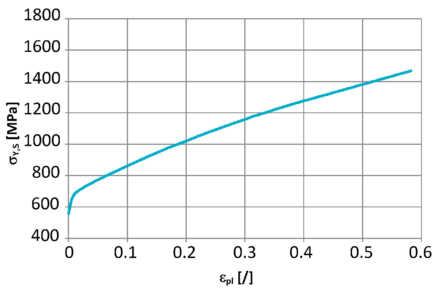
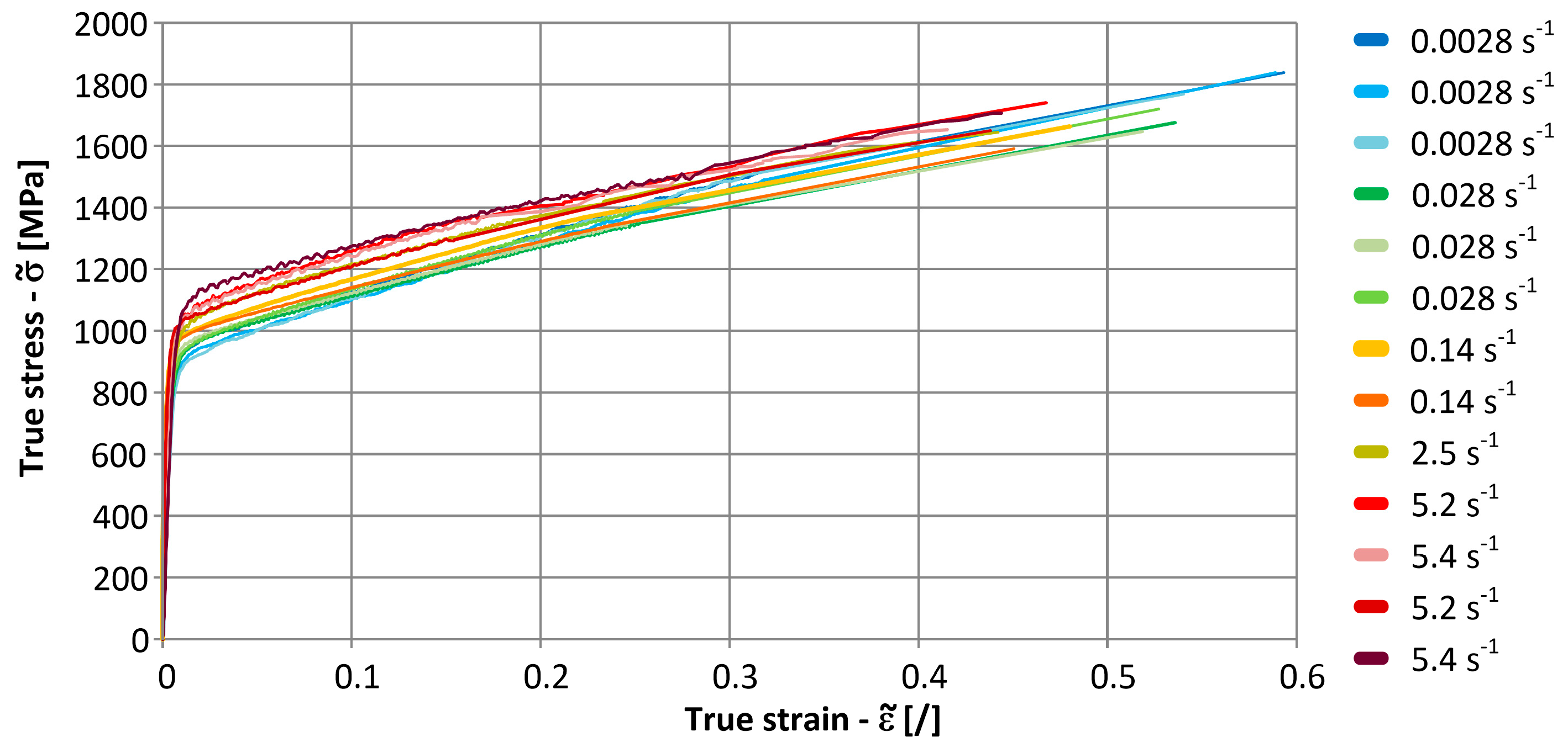
3.1. Tensile Stress-Strain Curves at Different Low-Strain Rates

Measured stress-strain diagrams for the low strain-rate tensile tests are presented in Figure 11. The average yield offset stress (Rp0.2) at the lowest strain rate and the ultimate tensile strength (Rm) from the tensile tests were approximately 800 MPa and 1100 MPa, respectively.
Due to different strain rate levels, different transformation methods were applied to obtain true stress-true strain curves from the engineering stress-strain curves in Figure 11. The measured engineering stress-strain curves at lower strain rates (below 0.14   s 1 ) were transformed into true stress-true strain curves according to the following equations [48]:
ε ˜ = l n ( 1 + ε )
σ ˜ = σ · ( 1 + ε )
ε and σ are the corresponding engineering strain and stress, respectively. This transformation is valid only before necking. After the tensile strength Rm of the material is reached, the true stress and true strain values should be calculated using the measured specimen cross-section at a specified sampling time. Along with the measured force at the same time, the true stress and true strain were calculated as follows:
ε ˜ = ln ( A 0 A )
σ ˜ = F A
A0 is an initial cross-section, and A and F are measured cross-section and force, respectively. Since it is difficult to perform the second part of the transformation manually during the experiment, the final true stress was determined only for the ruptured specimen, while the true strains were measured throughout the whole experiment using the high-speed camera combined with the DIC method. To estimate the true width of the specimen during the test, a tracking algorithm in ProAnalyst V1.8 software from Xcitex, Woburn, MA, USA, was applied.
At this point, it needs to be noted that for the highest strain rates between 2.5 s−1 and 5.4 s−1, the use of the mechanical extensometer was not a viable option. Consequently, only the strain data, which was determined with the DIC method, was available for these strain rates. For the lower strain rates, the strains from the DIC method were compared to the final strain from Equation (16) for the ruptured specimens as well as to the transformed values according to Equation (14) before the engineering tensile strength Rm was reached. It turned out that true strains were correctly determined using the DIC method. The obtained true stress-true strain curves are shown in Figure 12.

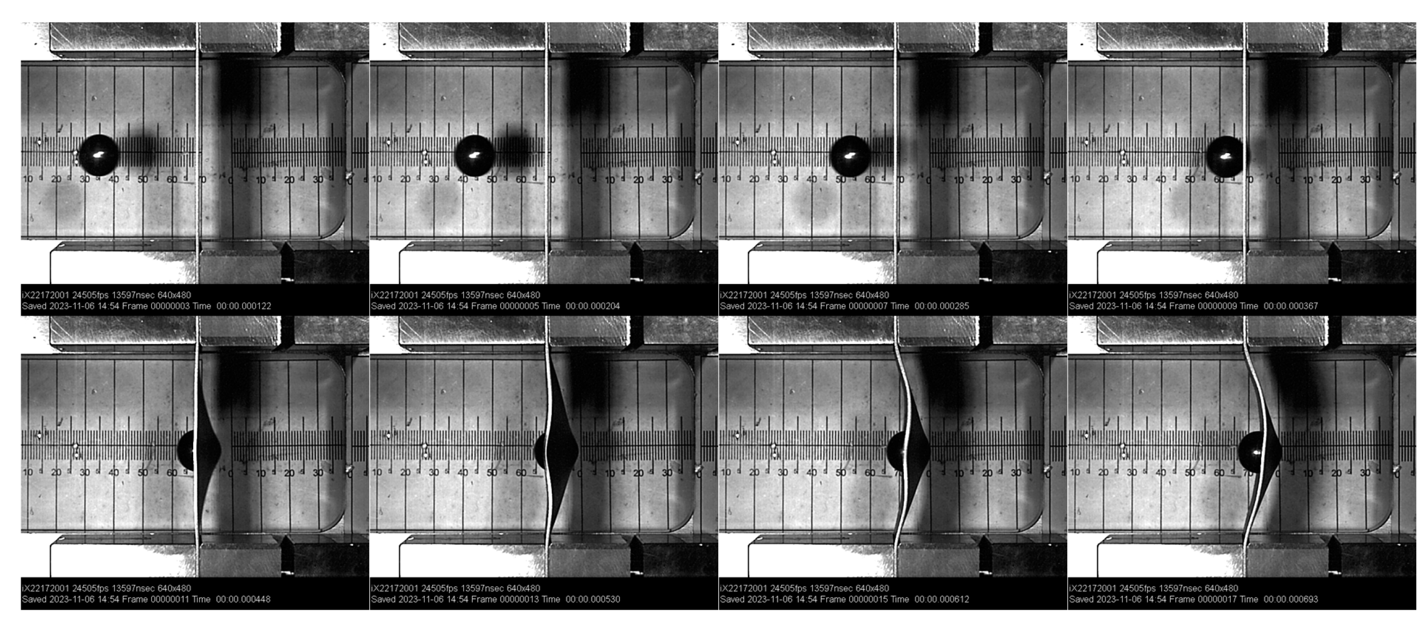
3.2. High Strain-Rate Experiments with a Shooting Ball Test

A sequence of figures from a single shooting ball test is presented in Figure 13. The combinations of the impact angle and impact velocity are presented in Table 4. The impact velocity of the ball was adjusted in such a manner that the plate-like specimen was significantly deformed, but the crack was not opened at the point of ball impact.

3.3. Estimating the Cowper–Symonds Parameters from the Experiments
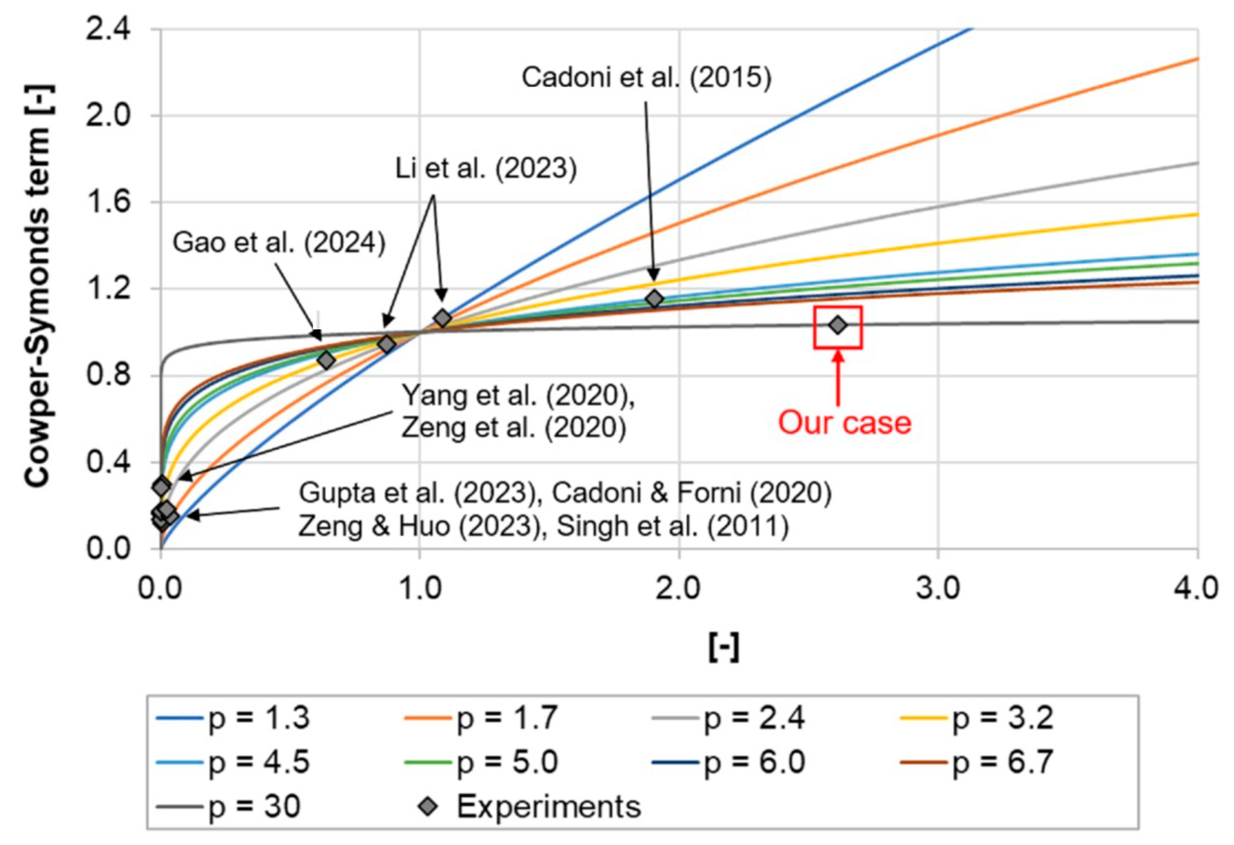
As already explained, the rough estimates of the three Cowper–Symonds parameters in Phase 1 were as follows: SIGY = 400 MPa, C = 210   s 1 , and p = 30 . The smoothed cost function SSQDLSR/1,000,000 for SIGY = 400 MPa and the ranges of the C and p parameters in Table 2 are presented in Figure 14.
A special note needs to be given here. After the comparison of this rough solution from Phase 1 to the known values of C and p parameters from the literature [18,20,22,23,25,27,28,30,32], we discovered that it is possible to obtain many almost optimal candidates in our case by varying the parameter SIGY and the height of the quasi-static flow stress curve. This could be implicated by a large plateau of the cost function SSQDLSR in Figure 14. The best two solutions among them (for differently high quasi-static flow stress curves, of course) were the following: (SIGY = 500 MPa, C = 300,000 s−1, p = 7) and (SIGY = 400 MPa, C = 210 s−1, p = 30). The corresponding cost function values, according to Equation (4), were almost identical (i.e., only 5% different). The first candidate solution was much closer to the values from the literature, as presented in Section 1. Then, we performed a rough reverse-engineering approach (i.e., a simplified version of Phase 2) for both candidate solutions using the LS-Dyna simulations. It turned out that the second candidate completely outperformed the first (more logical) one. Its cost function, according to Equation (13), was 30% smaller.
The key question arises: how could this happen? The answer lies in the mathematical formulation of the Cowper–Symonds term ( ε ˙ p l / C ) 1 / p . This is actually a power law (i.e., the root) function. Its examples for the two candidate solutions with p = 7 and p = 30 are presented in Figure 15. The strain rates at the shooting-ball test were between 300 s−1 and 450   s 1 . For the first optimum candidate ( S I G Y = 500   MPa ,     C = 300 , 000   s 1 ,   p = 7 ), it can be seen that the corresponding Cowper–Symonds term ( ε ˙ p l / C ) 1 / p is equal to 0.0015, which is very close to zero. This means that even a small variation in the strain rate results in a significant change of the term ( ε ˙ p l / C ) 1 / p . In contrast, the second optimum candidate ( S I G Y = 400   MPa ,   C = 210   s 1 ,   p = 30 ) is located to right of the (1,1) point in Figure 15. This means that the response of the term ( ε ˙ p l / C ) 1 / p to the variations of the strain rate is moderate and not abrupt, which is phenomenologically correct. Therefore, the parameter SIGY was kept constant at 400 MPa in Phase 2, because this was chosen as the most appropriate value in our case.
According to the methodology presented in Section 2.3, the SSQDHSR cost function was estimated for the high strain-rate experiments, and the multi-criterion MCF cost function was estimated that links together the results of the low- and high strain-rate experiments. The SSQDHSR cost function is presented in Figure 16, and the MCF cost function is presented in Figure 17. The optimum values of the Cowper–Symonds parameters, which were estimated using the RVGA, are C = 793.5 s−1 and p = 34.6. If Figure 14, Figure 16, and Figure 17 are compared, it can be concluded that the SSQDHSF cost function actually determines the final optimal values of the C and p parameters due to the large flat plateau of the cost function SSQDLSR. A comparison with the results from the literature is presented in Section 4.

4. Discussion

The optimal values of the parameters C and p are compared to the results, which were obtained by the other researchers [18,20,22,23,25,27,28,30,32]. As opposed to the usual comparisons in the form of data tables, the results from the literature are compared in the form of the Cowper–Symonds term ( ε ˙ p l / C ) 1 / p versus the ε ˙ p l / C parameter; see Figure 18. The values of the parameter p were taken from the references. It can be clearly seen from Figure 18 that more than half of the estimates from the literature are questionable. In most of these cases, the estimates of the parameter C are very high, i.e., C > 100,000. Since the measured strain rates were from the range of few 100 to a few 1000 in these cases, the corresponding values of the ε ˙ p l / C parameters are very near zero. As explained in Section 3.3, such estimates of the parameter C are phenomenologically suspicious, because even a small change of the strain rate results in a large change of the material’s response. This means that only four data points from the literature are more reliable, and three of them correspond to a value of the parameter p that is higher than its average from the literature. If we compare our results (C = 793.5 s−1 and p = 34.6) to these four reliable estimates from the literature, we can conclude that our estimates are reasonable for the available experimental data.
Such estimates, as can be found in the literature, are often a consequence of the following facts:
  • Most scholars applied the conventional formulation for the MAT_24 material, as shown in Equation (2), despite the fact that such a formulation is sometimes not appropriate for the studied steel alloys.
  • Furthermore, it is not optimal if the parameters C and p are estimated only on the basis of the high-strain rate experiments (e.g., Taylor test, split Hopkinson bar test, etc.). In the past [49], we also followed such an approach and obtained similar parameters. However, as soon as the optimisation process is extended to a wide range of strain rates, it turns out that the parameter values of C > 100,000 are not the best estimates. Despite the fact that different scholars have performed tests at different strain rates it is not clear how they considered the experimental data at various strain rates when estimating the parameters C and p.
If our estimates of the C and p parameters are compared to our previous research [15], it can be concluded that a similar value is obtained for the parameter p, but the estimate of the parameter C is now more than four-times higher, which puts our results closer to the reliable data from the literature. This is a confirmation that the procedure for estimating the Cowper–Symonds parameters from the high strain-rate experiments needs to be well-prepared and robust. We achieved this by replacing the point-wise comparison from Škrlec et al. [15] with the integral measure of deviation between the deformed specimen geometries from the high-strain-rate experiments and numerical simulations.
Last, but not least, a relatively high value of the parameter p means that the studied material is not sensitive to the strain rate effects. This is also not so unusual for the high-strength steel, because similar cases can be found in the literature [33,34,35].

5. Conclusions

Cowper–Symonds parameters were estimated for the complex-phase high-strength steel SZBS800 by performing a series of conventional tensile tests and unconventional high strain-rate experiments. The strain-rate dependent parameters C and p were estimated using a reverse engineering approach. The presented approach is an evolution of our previous research. The main novelty and innovation of this article is a definition of an integral cost function that measures a deviation between a deformed geometry of the flat specimens and the results of the numerical simulations. A DIC method, which is based on photographing the deformed specimens with triple cameras, is used for measuring the geometry of the deformed specimens. The parameter estimation is performed in two phases. LS-Dyna was used for numerical simulations in phase 2, and the material’s response was modelled using a piece-wise linear plasticity model with a visco-plastic formulation of the Cowper–Symonds material model. Finally, a multi-criteria cost function that combines the results of the low- and high-strain-rate experiments was defined and applied to obtain a response function for the parameters p and C. The results of this study can be summarised as follows:
  • The obtained results were compared to the values from the literature. It turned out that the estimated optimal values of the parameters C and p sometimes deviate significantly from the literature. After a careful analysis of our results and the published results from the literature, it can be concluded that some estimates in the literature are not very reliable due to different reasons that are explained in the article. This critical evaluation of our results and references presents another novelty of this article.
  • Yet another result of this study is a conclusion that it is immensely important is how the cost function is defined, which measures a deviation between the experimental results and numerical simulations for the high strain-rate experiments. It turns out that the integral measure of deviation is much better than the point-wise measure of deviation.
  • Finally, we can also conclude that the high-strength steel SZBS800 is not very sensitive to the strain, which is indicated by a rather high value of the Cowper–Symonds parameter p. However, such results are not surprising because it was previously discovered by other scholars that high-strength steels are often insensitive to the high strain-rate effects.

Author Contributions

Conceptualisation, A.Š., B.P., M.N. and J.K.; methodology, A.Š., B.P., M.N. and J.K.; software, A.Š., B.P., M.N. and J.K.; validation, A.Š., B.P., M.N. and J.K.; formal analysis, A.Š., B.P., M.N. and J.K.; investigation, A.Š., B.P., M.N. and J.K.; resources, A.Š., B.P., M.N. and J.K.; data curation, A.Š. and J.K.; writing—original draft preparation, A.Š., B.P., M.N. and J.K.; writing—review and editing, A.Š., B.P., M.N. and J.K.; visualisation, A.Š., B.P. and M.N.; supervision, M.N. and J.K.; project administration, M.N. and J.K.; funding acquisition, M.N. and J.K. All authors have read and agreed to the published version of the manuscript.

Funding

This research was funded by the Slovenian Research Agency (ARRS), grant research programme P2-0182 (R&D evaluations—Razvojna vrednotenja).

Data Availability Statement

The original contributions presented in the study are included in the article, further inquiries can be directed to the corresponding author.

Acknowledgments

The authors acknowledge support from the company TPV Automotive d.o.o. for the donation of the materials for testing.

Conflicts of Interest

The authors declare no conflicts of interest.

References

  1. Hallquist, J.O. LS-DYNA Theoretical Manual; Livermore Software Technology Corporation: Livermore, CA, USA, 2006; Available online: https://lsdyna.ansys.com/manuals/ (accessed on 26 August 2024).
  2. Hallquist, J.O. LS-DYNA Keyword User’s Manual R11.0. Volume I; Livermore Software Technology Corporation: Livermore, CA, USA, 2018; Available online: https://lsdyna.ansys.com/manuals/ (accessed on 26 August 2024).
  3. Taylor, G. The Use of Flat-Ended Projectiles for Determining Dynamic Yield Stress I. Theoretical Considerations. Proc. R. Soc. Lond. Ser. A Math. Phys. Sci. 1948, 194, 289–299. [Google Scholar] [CrossRef]
  4. Rohr, I.; Nahme, H.; Thoma, K. Material Characterization and Constitutive Modelling of Ductile High Strength Steel for a Wide Range of Strain Rates. Int. J. Impact Eng. 2005, 31, 401–433. [Google Scholar] [CrossRef]
  5. Deng, Y.; Wu, H.; Zhang, Y.; Huang, X.; Xiao, X.; Lv, Y. Experimental and Numerical Study on the Ballistic Resistance of 6061-T651 Aluminum Alloy Thin Plates Struck by Different Nose Shapes of Projectiles. Int. J. Impact Eng. 2022, 160, 104083. [Google Scholar] [CrossRef]
  6. Hopkinson, B.X. A Method of Measuring the Pressure Produced in the Detonation of High, Explosives or by the Impact of Bullets. Philos. Trans. R. Soc. Lond. Ser. A Contain. Pap. A Math. Or Phys. Character 1914, 213, 437–456. [Google Scholar] [CrossRef]
  7. Chen, W.; Song, B. Split Hopkinson (Kolsky) Bar: Design, Testing and Applications; Mechanical Engineering Series; Springer: Boston, MA, USA, 2011; ISBN 978-1-4419-7981-0. [Google Scholar]
  8. Forni, D.; Mazzucato, F.; Valente, A.; Cadoni, E. High Strain-Rate Behaviour of as-Cast and as-Build Inconel 718 Alloys at Elevated Temperatures. Mech. Mater. 2021, 159, 103859. [Google Scholar] [CrossRef]
  9. Meyers, M.A. Dynamic Behavior of Materials, 1st ed.; Wiley: Hoboken, NJ, USA, 1994; ISBN 978-0-471-58262-5. [Google Scholar]
  10. Froustey, C.; Lambert, M.; Charles, J.L.; Lataillade, J.L. Design of an Impact Loading Machine Based on a Flywheel Device: Application to the Fatigue Resistance of the High Rate Pre-Straining Sensitivity of Aluminium Alloys. Exp. Mech. 2007, 47, 709–721. [Google Scholar] [CrossRef]
  11. Meram, A. Dynamic Characterization of Elastomer Buffer under Impact Loading by Low-Velocity Drop Test Method. Polym. Test. 2019, 79, 106013. [Google Scholar] [CrossRef]
  12. Hernandez, C.; Buchely, M.F.; Maranon, A. Dynamic Characterization of Roma Plastilina No. 1 from Drop Test and Inverse Analysis. Int. J. Mech. Sci. 2015, 100, 158–168. [Google Scholar] [CrossRef]
  13. Song, B.; Sanborn, B.; Heister, J.; Everett, R.; Martinez, T.; Groves, G.; Johnson, E.; Kenney, D.; Knight, M.; Spletzer, M. Development of “Dropkinson” Bar for Intermediate Strain-Rate Testing. EPJ Web Conf. 2018, 183, 02004. [Google Scholar] [CrossRef]
  14. Othman, R.; Guégan, P.; Challita, G.; Pasco, F.; LeBreton, D. A Modified Servo-Hydraulic Machine for Testing at Intermediate Strain Rates. Int. J. Impact Eng. 2009, 36, 460–467. [Google Scholar] [CrossRef]
  15. Škrlec, A.; Kocjan, T.; Nagode, M.; Klemenc, J. Modelling a Response of Complex-Phase Steel at High Strain Rates. Materials 2024, 17, 2302. [Google Scholar] [CrossRef] [PubMed]
  16. D20 Committee. Test Method for Impact Resistance of Flat, Rigid Plastic Specimen by Means of a Striker Impacted by a Falling Weight (Gardner Impact); ASTM International: West Conshohocken, PA, USA, 2007. [Google Scholar]
  17. GB/T 1591-2018; High Strength Low Alloy Structural Steels (English Version). SAMR, SAC: Beijing, China, 2018.
  18. Li, H.; Li, F.; Zhang, R.; Zhi, X. High Strain Rate Experiments and Constitutive Model for Q390D Steel. J. Constr. Steel Res. 2023, 206, 107933. [Google Scholar] [CrossRef]
  19. EN 10088-4:2009; Stainless Steels—Part 4: Technical Delivery Conditions for Sheet/Plate and Strip of Corrosion Resisting Steels for Construction Purposes. Technical Committee ECISS/TC 105. CEN Management Centre: Brussels, Belgium, 2009.
  20. Gupta, M.K.; Singh, N.K.; Gupta, N.K. Deformation Behaviour and Notch Sensitivity of a Super Duplex Stainless Steel at Different Strain Rates and Temperatures. Int. J. Impact Eng. 2023, 174, 104494. [Google Scholar] [CrossRef]
  21. EN 10025-6:2019; Hot Rolled Products of Structural Steels—Part 6: Technical Delivery Conditions for Flat Products of High Yield Strength Structural Steels in the Quenched and Tempered Condition. Technical Committee ECISS/TC 103. CEN Management Centre: Brussels, Belgium, 2019.
  22. Yang, X.; Yang, H.; Lai, Z.; Zhang, S. Dynamic Tensile Behavior of S690 High-Strength Structural Steel at Intermediate Strain Rates. J. Constr. Steel Res. 2020, 168, 105961. [Google Scholar] [CrossRef]
  23. Cadoni, E.; Forni, D. Strain-Rate Effects on S690QL High Strength Steel under Tensile Loading. J. Constr. Steel Res. 2020, 175, 106348. [Google Scholar] [CrossRef]
  24. EN 10083-3:2006; Steels for Quenching and Tempering—Part 3: Technical Delivery Conditions for Alloy Steels. Technical Committee ECISS/TC 105. CEN Management Centre: Brussels, Belgium, 2006.
  25. Gao, S.; Yu, X.; Li, Q.; Sun, Y.; Hao, Z.; Gu, D. Research on Dynamic Deformation Behavior and Constitutive Relationship of Hot Forming High Strength Steel. J. Mater. Res. Technol. 2024, 28, 1694–1712. [Google Scholar] [CrossRef]
  26. DGJ32/TJ 202-2016; Technical Specification for Application of Heat-Treatment High-Strength Ribbed Bar in Concrete Structures. Jiangsu Phoenix Science and Technology Press: Nanjing, China, 2016.
  27. Zeng, X.; Huo, J.S. Rate-Dependent Constitutive Model of High-Strength Reinforcing Steel HTRB600E in Tension. Constr. Build. Mater. 2023, 363, 129824. [Google Scholar] [CrossRef]
  28. Singh, N.K.; Cadoni, E.; Singha, M.K.; Gupta, N.K. Dynamic Tensile Behavior of Multi Phase High Yield Strength Steel. Mater. Des. 2011, 32, 5091–5098. [Google Scholar] [CrossRef]
  29. EN 1992-1-1:2005; Eurocode 2: Design of Concrete Structures—Part 1-1: General Rules and Rules for Buildings. Technical Committee CEN/TC 250. CEN Management Centre: Brussels, Belgium, 2004.
  30. Cadoni, E.; Dotta, M.; Forni, D.; Tesio, N. High Strain Rate Behaviour in Tension of Steel B500A Reinforcing Bar. Mater. Struct. 2015, 48, 1803–1813. [Google Scholar] [CrossRef]
  31. GB/T 1499.2-2018; Steel for the Reinforcement of Concrete—Part 2: Hot Rolled Ribbed Bars (English Version). AQSIQ, SAC: Beijing, China, 2018.
  32. Zeng, X.; Huo, J.; Wang, H.; Wang, Z.; Elchalakani, M. Dynamic Tensile Behavior of Steel HRB500E Reinforcing Bar at Low, Medium, and High Strain Rates. Materials 2020, 13, 185. [Google Scholar] [CrossRef]
  33. Nahme, H.; Lach, E. Dynamic Behavior of High Strength Armor Steels. Le J. De Phys. IV 1997, 7, C3–C373. [Google Scholar] [CrossRef]
  34. Børvik, T.; Hopperstad, O.S.; Dey, S.; Pizzinato, E.V.; Langseth, M.; Albertini, C. Strength and Ductility of Weldox 460 E Steel at High Strain Rates, Elevated Temperatures and Various Stress Triaxialities. Eng. Fract. Mech. 2005, 72, 1071–1087. [Google Scholar] [CrossRef]
  35. Trajkovski, J.; Kunc, R.; Pepel, V.; Prebil, I. Flow and Fracture Behavior of High-Strength Armor Steel PROTAC 500. Mater. Des. 2015, 66, 37–45. [Google Scholar] [CrossRef]
  36. Huang, Y.H. Shape Measurement by the Use of Digital Image Correlation. Opt. Eng. 2005, 44, 087011. [Google Scholar] [CrossRef]
  37. Aktepe, R.; Guldur Erkal, B. State-of-the-Art Review on Measurement Techniques and Numerical Modeling of Geometric Imperfections in Cold-Formed Steel Members. J. Constr. Steel Res. 2023, 207, 107942. [Google Scholar] [CrossRef]
  38. Tarigopula, V.; Hopperstad, O.S.; Langseth, M.; Clausen, A.H.; Hild, F. A Study of Localisation in Dual-Phase High-Strength Steels under Dynamic Loading Using Digital Image Correlation and FE Analysis. Int. J. Solids Struct. 2008, 45, 601–619. [Google Scholar] [CrossRef]
  39. Tiwari, V.; Sutton, M.A.; McNeill, S.R.; Xu, S.; Deng, X.; Fourney, W.L.; Bretall, D. Application of 3D Image Correlation for Full-Field Transient Plate Deformation Measurements during Blast Loading. Int. J. Impact Eng. 2009, 36, 862–874. [Google Scholar] [CrossRef]
  40. Borkowski, Ł.; Grudziecki, J.; Kotełko, M.; Ungureanu, V.; Dubina, D. Ultimate and Post-Ultimate Behaviour of Thin-Walled Cold-Formed Steel Open-Section Members under Eccentric Compression. Part II: Experimental Study. Thin-Walled Struct. 2022, 171, 108802. [Google Scholar] [CrossRef]
  41. Shin, W.; Yoo, C. Application of the Digital Image Correlation Technique in Wide Width Tensile Test of Geogrids. Geotext. Geomembr. 2024, 52, 1087–1098. [Google Scholar] [CrossRef]
  42. SZBS800 Multiphase Steels: Bainitic Grade. Salzgitter Flachstahl GmbH. Available online: https://www.salzgitter-flachstahl.de/fileadmin/footage/media/gesellschaften/szfg/informationsmaterial/produktinformationen/warmgewalzte_produkte/eng/szbs800.pdf (accessed on 26 February 2024).
  43. E28 Committee. Test Methods for Tension Testing of Metallic Materials; ASTM International: West Conshohocken, PA, USA, 2011. [Google Scholar]
  44. Rolling Elements|Schaeffler Medias. Available online: https://medias.schaeffler.hu/en/rolling-elements (accessed on 23 August 2024).
  45. EN-ISO 683-17:2023(En); Heat-Treated Steels, Alloy Steels and Free-Cutting Steels—Part 17: Ball and Roller Bearing Steels. ISO: Geneva, Switzerland, 2023.
  46. Besseling, J.F. A Theory of Elastic, Plastic, and Creep Deformations of an Initially Isotropic Material Showing Anisotropic Strain-Hardening, Creep Recovery, and Secondary Creep. J. Appl. Mech. 1958, 25, 529–536. [Google Scholar] [CrossRef]
  47. Škrlec, A.; Klemenc, J. Estimating the Strain-Rate-Dependent Parameters of the Johnson-Cook Material Model Using Optimisation Algorithms Combined with a Response Surface. Mathematics 2020, 8, 1105. [Google Scholar] [CrossRef]
  48. Mirone, G.; Barbagallo, R.; Bua, G.; De Caro, D.; Ferrea, M.; Tedesco, M.M. A Simple Procedure for the Post-Necking Stress-Strain Curves of Anisotropic Sheet Metals. Metals 2023, 13, 1156. [Google Scholar] [CrossRef]
  49. Škrlec, A.; Klemenc, J. Estimating the Strain-Rate-Dependent Parameters of the Cowper-Symonds and Johnson-Cook Material Models Using Taguchi Arrays. Stroj. Vestn. J. Mech. Eng. 2016, 62, 220–230. [Google Scholar] [CrossRef]
Figure 1. Flat specimen for tensile tests according to ASTM E8/E8M standard (Reprinted from [43]) (all presented dimensions are in mm).
Metals 14 00992 g001
Figure 2. Experimental setup for measuring the deformed geometry of the specimens with the Dantec 3D DIC system.
Metals 14 00992 g002
Figure 3. Conventional Cowper–Symonds model in LS-Dyna software.
Metals 14 00992 g003
Figure 4. Visco-plastic formulation of the strain-rate-dependent flow curve in LS-Dyna software.
Metals 14 00992 g004
Figure 5. Used flow curve σ Y , S ( ε p l ) at quasi-static strain rates.
Metals 14 00992 g005
Figure 6. Deformed geometry of the plate-like specimen in mm from LS-Dyna simulations.
Metals 14 00992 g006
Figure 7. Results obtained from impact simulations with LS-Dyna software. Colour bar represents the displacement values along y direction. (a) Results at initial timestamp before impact. (b) Results at final timestamp after impact.
Metals 14 00992 g007
Figure 8. Reference images for different image resolutions. (a) Using 2-times higher resolution than the original simulation. Coordinate increment was d x = d z = 0.3125 with matrix numbers of columns and rows, respectively n x = 192 , n z = 208 . (b) Using the original simulation resolution. Coordinate increment was d x = d z = 0.625 with matrix numbers of columns and rows, respectively n x = 96 , n z = 104 . (c) Using 2-times lower resolution than the original simulation. Coordinate increment was d x = d z = 1.25 with matrix numbers of columns and rows, respectively n x = 48 , n z = 59 . The colour scale is the same as in the Figure 7 and represents the displacement values along y direction.
Metals 14 00992 g008
Figure 9. DIC references images for different image resolutions. (a) Using a 2-times higher resolution than the original DIC mesh size. Coordinate increment was d x = d z = 0.25 with matrix numbers of columns and rows, respectively n x = 333 , n z = 466 . (b) Using the original simulation resolution as DIC mesh size. Coordinate increment was d x = d z = 0.5 with matrix numbers of columns and rows, respectively n x = 167 , n z = 233 . (c) Using a 2-times lower resolution than the original DIC mesh size. Coordinate increment was d x = d z = 1 with matrix numbers of columns and rows, respectively n x = 84 , n z = 117 . The colour scale is the same as in the Figure 7 and represents the displacement values along y direction.
Metals 14 00992 g009
Figure 10. DIC reference images with cropping rectangles. (a) DIC reference image with 2-times higher resolution. (b) DIC reference image with original resolution. (c) DIC reference image with 2-times lower resolution. The colour scale is the same as in the Figure 7 and represents the displacement values along y direction.
Metals 14 00992 g010
Figure 11. Measured stress-strain diagrams for the low strain-rate tensile tests.
Metals 14 00992 g011
Figure 12. True stress—true strain curves for low strain-rate tensile tests.
Metals 14 00992 g012
Figure 13. Ball motion during the high strain-rate experiments.
Metals 14 00992 g013
Figure 14. Smoothed SSQDLSR cost function for the low strain-rate experiments.
Metals 14 00992 g014
Figure 15. Cowper–Symonds relationships for different values of the parameter p.
Metals 14 00992 g015
Figure 16. Smoothed SSQDHSR cost function for the high strain rate experiments.
Metals 14 00992 g016
Figure 17. Smoothed MCF multi-criteria cost function.
Metals 14 00992 g017
Figure 18. Comparison of our results to the literature data (Adapted from [18,20,22,23,25,27,28,30,32]).
Metals 14 00992 g018
Table 1. Chemical composition of SZBS800 steel (Adapted from [42]).
CSiMnPSAlBCu
max.max.max.max.max.min.max.max.
0.18%1.00%2.20%0.05%0.01%0.015–1.2%0.005%0.2%
In addition, the elements Nb, V, and Ti are each alloyed either individually or in combination (Nb + V + Ti ≤ 0.25%). Fe accounts for the rest of the share.
Table 2. Division for the parameters C and p.
ParameterValues
C [s−1]10, 30, 50, 70, 90, 1110, 130, 150, 170, 190, 210, 230, 250, 270, 300, 600
p [/]10, 15, 20, 25, 30, 40, 50, 60, 70, 80, 90, 100
Table 3. Division of the parameters C and p for the LS-DYNA simulations.
ParameterValues
C [s−1]70, 150, 230, 310, 390, 470, 550, 630, 710, 790,
870, 950, 1030, 1110, 1190, 1270, 1350
p [/]15, 20, 25, 30, 35, 40, 45
Table 4. Boundary conditions for the shooting ball experiments.
ParameterValues
Impact angles α [°]0, 0, 0, 20, 20, 20, 35, 35, 35
Impact velocity v [m/s]111.5, 133.3, 155.3, 111.2, 132.6, 154.2, 113.1, 131.9, 153.5
Disclaimer/Publisher’s Note: The statements, opinions and data contained in all publications are solely those of the individual author(s) and contributor(s) and not of MDPI and/or the editor(s). MDPI and/or the editor(s) disclaim responsibility for any injury to people or property resulting from any ideas, methods, instructions or products referred to in the content.

