
Investigation of Indirect Shear Strength of Black Shale for Urban Deep Excavation


School of Civil, Environmental, and Architectural Engineering, Korea University, Seoul 02841, Republic of Korea
Buildings 2024, 14(10), 3050; https://doi.org/10.3390/buildings14103050
Submission received: 31 August 2024
/
Revised: 20 September 2024
/
Accepted: 23 September 2024
/
Published: 24 September 2024
(This article belongs to the Special Issue Advances in Foundation Engineering for Building Structures)
Abstract
:This study thoroughly investigated the compressive and tensile strength characteristics of black shale using both experimental and analytical approaches. Uniaxial compression tests were conducted to determine the elastic constants of black shale modeled as idealized, linear elastic, homogeneous, and transversely isotropic. Additionally, Brazilian tests were carried out on shale, considering it a transversely isotropic material. Strain measurements were recorded at the center of disc specimens subjected to diametric loading. By placing strain gages at the disc centers, the five elastic constants were accurately estimated. The effects of experimental methods and diametric loading on the elastic constant determination were evaluated and analyzed, and the indirect shear strength of the black shale, considering anisotropy, was determined using the estimated stress concentration coefficient. This study revealed that the indirect tensile strength of black shale is significantly influenced by the angle between the anisotropic planes and the diametric loading direction. Moreover, it was revealed that the stress concentration coefficients for anisotropic rocks vary from those of isotropic rocks, depending on the inclination angle of the bedding planes. This study confirms that the shear (tensile) strength of anisotropic black shale is not constant but varies with the orientation of the anisotropic planes in relation to the applied load.
1. Introduction
Recently, in response to the saturation of ground structures in urban areas and severe traffic congestion, the importance of developing underground spaces, such as roadways, underground railways, and metropolitan areas, has become increasingly apparent. Case studies on deep excavation are being reported in many European and Asian countries [1,2,3,4,5,6,7]. Additionally, the development of underground spaces using tunnels is actively progressing at various sites in the Republic of Korea [8,9]. This development offers several advantages, including the expansion of transportation infrastructure, the creation of additional commercial and residential spaces, and enhancement of cities’ functional efficiency. Specifically, underground structures like subways, tunnels, and parking lots play a crucial role in reducing surface-level congestion and facilitating smoother traffic flow. Therefore, understanding rock characteristics is essential for developing rock areas and ensuring the stability of underground structures [10,11,12].
Many rocks exhibit structural features such as bedding, layering, stratification, jointing, or fissuring [13,14]. These features often result in directional variability in their properties—whether physical, dynamic, thermal, mechanical, or hydraulic—causing the rocks to be naturally anisotropic [15]. Anisotropy can occur at various scales, ranging from individual samples to entire rock formations. This phenomenon is commonly seen in intact foliated metamorphic rocks, as well as in stratified, laminated, and sedimentary rocks. On a larger scale, anisotropy may also be evident in volcanic formations, sedimentary layers containing alternating rock types, and formations intersected by one or more sets of regularly spaced joints [16,17,18,19].
The anisotropy of rocks is a critical factor in geotechnical engineering, influencing the stability of both underground and ground excavations, as well as the performance of foundations in urban deep excavation projects. It is also critical in various processes, such as drilling, blasting, rock cutting, and the propagation of fractures. On construction sites characterized by discontinuities like faults, fractures, joints, and bedding planes, tensile strength often becomes more important than compressive or shear strength. Despite its significance, rock anisotropy is not fully understood, particularly in practical applications. Accurately characterizing the anisotropy of rocks, whether in the laboratory or in situ, continues to be a significant challenge.
In laboratory settings, the engineering properties of anisotropic rock materials are usually assessed by performing tests with samples that are prepared in different orientations in relation to the visible anisotropic planes. According to previous studies [17,20], testing methods are generally categorized into static and dynamic approaches. Static methods involve uniaxial, triaxial, and multi-axial compressive tests, indirect shear (Brazilian) tests, hollow cylinder tests, as well as torsion and bending tests. In addition, dynamic methods include approaches such as the resonant bar technique and the ultrasonic wave technique. The process of preparing test specimens, including their dimensions and the minimum number needed to assess anisotropic rock properties, typically depends on the specific testing method used. Among these methods, the Brazilian test, which involves diametral loading of rock discs, is particularly notable for its less demanding specimen preparation requirements and the relatively straightforward analysis of its results.
The anisotropy impact on tensile strength determined by the indirect shear (Brazilian) test has been widely studied across various materials, such as coal, metamorphic rocks, and sedimentary rocks [21,22,23,24,25,26]. These studies generally observed that test samples failed along the diametric load, regardless of the orientation of the anisotropic layers within the rocks. Indirect tensile strength was generally calculated using an equation derived from isotropic elasticity theory, despite the rocks displaying anisotropic characteristics. For estimating deformability, the Brazilian test has been used to calculate Young’s modulus and Poisson’s ratio of concrete samples under the assumption of isotropic behavior [27]. This approach was adapted to evaluate Young’s modulus and Poisson’s ratio for schist disc samples by extending Hondros’s method [22], which was initially intended for isotropic rock samples [28]. In Loureiro-Pinto’s adaptation [27], it was assumed that the stress intensity at the center of an anisotropic rock disc sample would be the same as that in an isotropic disc—this assumption holds only when the disc is aligned parallel to a plane of transverse isotropy. For all other orientations, anisotropy must be accounted for. Loureiro-Pinto’s approach was enhanced, and a method was devised to assess the five elastic constants of transversely isotropic rocks [29], although this method did not incorporate thermodynamic conditions [30]. To address this problem, the elastic constants were derived from uniaxial compression tests. To do that, strain data from Brazilian tests were used to solve a system of constrained equations through a constrained optimization technique [31,32]. The complex stress function method has been employed to connect stresses and strains in a thin disc of anisotropic material under diametric loading [33]. This method has also been applied to evaluation of the indirect shear (tensile) strength of rocks with anisotropy, proving effective in such assessments [33,34,35].
This paper integrates both experimental and analytical methods to assess the characteristics of transversal isotropic rocks in a controlled laboratory environment. Particularly, it aims to evaluate the indirect tensile strength of rocks by utilizing Brazilian tests on black shale, which is assumed to exhibit transverse isotropy. The research aims to evaluate the deformability and tensile strength of shale through both analytical and experimental approaches. Numerical analysis using the Finite Element Method (FEM) was conducted, complemented by experimental data collected from shale samples. The stress concentration coefficients obtained through this method were compared with those derived from experimental results on the same rock specimens. This study sought to enhance understanding of the engineering properties of transversely isotropic rocks, particularly their deformability and indirect tensile strength, and to assess the impact of rock anisotropy on tensile strength under different loading conditions. By addressing the challenges of accurately characterizing rock anisotropy in the laboratory, this research aims to improve the stability and safety of engineering projects involving anisotropic rock formations.
2. Elastic Equilibrium of Anisotropic Medium
In Figure 1, a thin, homogeneous, linear elastic disc sample within a transversely isotropic medium is considered. The disc sample features a diameter (D) and a thickness (t), with the angle (ψ) indicating its inclination. The components Xn and Yn are the surface forces per unit area along the disc’s edge in the x and y directions, respectively, and these forces are considered to be in a state of equilibrium. In addition, the symbol “ω” represents the angular displacement or rotation about the horizontal axis, specifically the x-axis. In this context, ω refers to the rotational movement about this axis, which is a common notation in rotational mechanics and kinematic descriptions of rigid body motion. If we assume that the sample lies parallel to the middle plane, is subjected to surface forces, and experiences only small deformations, a generalized plane stress approach can be applied.
If we assume that the disc sample lies parallel to the middle plane, is subjected to surface forces, and experiences only small deformations, a generalized plane stress approach can be applied. The material’s constitutive relation in the x–y plane is given in Equation (1).
Here, the compliance components (i.e., , …, ) are computed in the x and y coordinates. The components are influenced by the inclination angle (ψ) and elastic constants defined in the coordinates (i.e., x′, y′, and z′). For transversal isotropy of material, there are five independent elastic constants, denoted in this study as E, E′, v, v′, and G′. Young’s modulus, represented by E, pertains to the stiffness within the transverse isotropic plane, while E’ refers to the modulus in the direction perpendicular to this plane. The Poisson’s ratios, v and v′, describe the horizontal strain response within the transverse isotropic plane, with v corresponding to the stress applied parallel to the plane and v′ to the stress applied perpendicular to it. G′ represents the shear modulus in planes that are perpendicular to the transverse isotropic plane, whereas the shear modulus (G) within the plane of transverse isotropy is dependent and can be calculated as E/2(1 + v). By applying coordinate transformation directions, it can be demonstrated that for the geometry depicted in Figure 1, the compliance components do not depend on Poisson’s ratio and are related to the five elastic constants as outlined in Equations (2)–(7).
Let F be defined as stress such that the stress components (σx, σy, and τxy) are expressed in terms of the second partial derivatives of E concerning the spatial coordinates x and y, as shown in Equation (8).
Figure 2 describes the diametric compression of the disc samples subjected to loading over an angular width of 2α in the transverse isotropic plane and the plane perpendicular to the transverse isotropic plane.
The angle of loading (2α) is considered to be sufficiently small so that p can be approximated as W/(αDt), where W represents the load applied on the disc sample on the y-axis. Under these boundary conditions, it can be demonstrated that the stress components at any points (x, y) within the sample can be expressed as shown in Equation (9).
The stress concentration coefficients (i.e., , , and ) are functions of the coordinates (x and y) at the point of interest, the loading angle (2α), and the compliance components (, , , , , and ). As indicated in Equations (2)–(7), these coefficients are affected by the inclination angle (ψ) and the elastic constant ratios (i.e., E/E′, E/G′, and v′). Replacing Equation (9) in Equation (1) results in the expression presented in Equation (10).
The elastic constants of rocks evaluated as a transversal isotropic material can be determined. First, Equation (10) can be used to calculate the five elastic constants from the strains measured at the center of a disc subjected to a diametric load, as described in Figure 2a,b. Then, a disc sample with its midplane parallel to the transversal isotropic plane (Figure 2a) is utilized to estimate the elastic constants (i.e., E and v) for isotropy. The stress concentration coefficients (ζxx, ζyy, and ζxy) can be evaluated based on the half-loading strip angle for this orientation. After applying the selected concentration coefficients in Equation (10), it can be rewritten as Equation (11).
By taking the longitudinal strain measurements on the plane in at least two different non-parallel axes, Equation (11) can be applied to evaluate both elastic constants (E and v).
Another disc sample with its mid-plane perpendicular to the transversal isotropic plane (Figure 2b) is utilized to evaluate the other elastic constants (E′, ν′, and G′). This allows Equation (10) to be rewritten as Equation (12),
where A1, A2, A3, K11, …, K33 are functions of ζxx, ζyy, and ζxy and the angle ψ. When choosing the elastic constants for a transversal isotropic material, thermodynamic conditions must be fulfilled [29,36]. Equation (12) describes a complicated nonlinear matrix involving three variables (1/E′, ν′/E′, and 1/G′), which must fulfill the limitations outlined in Equation (13). Equation (13) provides a thermodynamic stability condition that must be satisfied when choosing the elastic constants for a transversely isotropic material, ensuring that the selected material properties are physically meaningful.
3. Materials and Methods
3.1. Properties of Black Shale
Figure 3 presents the geological map of the area, with the marked section indicating the location where the samples used in this study were collected. The sample, black shale, belongs to the sedimentary rocks of the Haman Formation (Fm.) in Daegu, Republic of Korea. In the laboratory, a specific gravity test, as well as basic physical property tests (e.g., water content, saturation, porosity, and absorption rate), was carried out. In general, specific gravity is physically defined as the ratio of the mass of a sample to the mass of an equal volume of pure water at 4 °C, measured under 1 atmosphere of pressure. Specific gravity can be categorized into true specific gravity, apparent specific gravity, and volumetric specific gravity. Among these methods, the most commonly used is the apparent specific gravity method. Therefore, specific gravity tests in the natural, dry, and saturated states were conducted, and the results, along with basic physical properties, are summarized in Table 1. The specific gravity values for the natural, dry, and saturated states were 2.717, 2.702, and 2.722, respectively. In addition, the natural water content (wn) ranged from 0.16% to 0.65%, the natural saturation (Sr) ranged from 59.57% to 7.65%, the effective porosity (ne) was between 0.75% and 3.74%, and the absorption rate (ab) ranged from 0.26% to 0.78%.
The engineering properties of rocks are directly influenced by factors such as mineral and chemical composition, particle structure, and arrangement. Qualitative analysis of clay minerals or non-clay minerals is typically conducted through X-ray powder diffraction, along with chemical analysis and examination using electron microscopy. In this study, X-ray diffraction (XRD) tests were conducted at the Daegu Branch of the Korea Basic Science Institute for this qualitative analysis. Table 2 shows the quantitative values obtained from the constituent minerals, revealing that the black shale in this region is primarily composed of a large amount of clay minerals (Cm), quartz (Q), feldspar (albite, Ab), and calcite (Cc). Figure 4 presents the results of an X-ray diffraction experiment and a photograph of a scanning electron microscope (SEM) analysis of black shale. The SEM image shows a granular and porous microstructure, which is consistent with the mineral composition indicated in the XRD plot. The presence of quartz as the dominant mineral (as shown by the sharp peak) correlates with the visible granular texture in the SEM, while the clay minerals like chlorite, though less dominant, could be responsible for the more compact regions in the image.
3.2. Uniaxial Compression Test
In this study, nine uniaxial compression tests were performed using an MTS machine with a load capacity of 996.4 kN (100 tons), and the load was applied at a rate of 1.5 mm per minute (strain control). All specimens were subjected to loading until failure, and the failure loads were measured. The sample preparation and the testing procedures followed the guidelines established by the International Society for Rock Mechanics and Rock Engineering (ISRM).
Figure 5 presents the appearance of the samples after preparation for the uniaxial compression test. The rock samples were carefully selected to minimize heterogeneity, focusing on rock forms with regular stratification intervals to account for anisotropic characteristics. The rock cores, drilled with a 54 mm diameter core drill, were oriented so that the stratification planes formed angles (θ) of 0°, 45°, and 90° relative to the main loading surface. The load was applied vertically along the y-axis, with strain gages symmetrically positioned to measure strains in both the x and y directions. Each strain gage was 5 mm long, had a resistance of 120 Ω, and was attached to the center of the specimens along the x and y axes.
The five elastic constants were determined at 50% of the breaking load based on the measurements obtained from the three samples prepared at different orientations (0°, 45°, and 90°). The angle θ refers to the inclination angle of the transversal isotropic plane in the rock. Strains measured from specimens with θ = 0° (Figure 5a) were used to calculate E′ and v′, while strains from specimens with θ = 90° (Figure 5b) provided values for E and v. Specimens with θ = 45° (Figure 5c) were utilized to assess the shear modulus (G’).
3.3. Indirect Tensile Strength (Brazilian Test)
Figure 6 shows a sample with strain gages attached for loading in the horizontal direction on the transverse isotropic surface and samples after attaching the strain gages when the angles between the horizontal plane and the floor surface were ψ = 0°, 15°, 30°, 45°, 60°, 75°, and 90°.
For the Brazilian test, the rock core sample was drilled with its diameter aligned at 0° and 90° relative to the main pressing surface, using a coring drill. The thickness of disc samples was 25 mm in both the horizontal direction on the floor surface and the direction perpendicular to the floor surface. As shown in Figure 2a, when a load is applied horizontally on the transverse isometric surface (loading rate = 0.025 mm/s), and the load angle (2α) is less than 15°, the stress concentration coefficient at the sample’s center is estimated to be similar to that of an isotropic material. The strain gauges were attached in the x and y directions. The strain measured at 50% of the load at failure was used to calculate the coefficient at the sample’s center and compare it with that of an isotropic material.
To evaluate the stress concentration coefficients for each angle when loading a disc sample in a perpendicular direction to the transversal isotropic plane, as shown in Figure 2b, disc samples with ψ angles of 0°, 15°, 30°, 45°, 60°, 75°, and 90° were prepared—three for each angle. Three strain gauges were attached in the x, y, and 45° axes to measure the strain until the sample failed. The load was applied during the test using the same MTS system employed for the uniaxial compression tests; the stress concentration coefficient at the sample’s center was calculated using the strain measured at 50% of the breaking load. The indirect tensile strength for each angle was determined using the stress concentration coefficient obtained from 50% of the failure load.
The process for the elastic constant evaluation of each of the black shale samples through diametric loading involved several steps. Initially, two types of disc samples were made. The first type, with the midplane either perpendicular or parallel to the transversal isotropic plane (Figure 2a), was utilized to evaluate the elastic constants (i.e., E and ν) for isotropy. The second type, with the midplane either parallel or perpendicular to the transversal isotropic plane (Figure 2b), was utilized to calculate the remaining elastic constants (i.e., E′, ν′, and G′). Axial strains were then measured in the horizontal, vertical, and 45° directions by attaching a 45° strain gauge at the core of each disc sample. Diametric loading was applied using two steel plates over an arc defined by the contact angle 2α, with each disc sample loaded vertically until failure. The five constants were subsequently calculated from the strains measured using Equations (6)–(8). Lastly, the indirect tensile strength of each black shale sample was determined by measuring the failure load of the indirect shear (Brazilian) tests and applying the horizontal stress formula from Equation (4).
4. Results and Discussions
4.1. Results of Uniaxial Compression Test
Figure 7 presents the results of the uniaxial compression test on the black shale from Daegu, Republic of Korea. In addition, as previously described, the five elastic constants (E, v, E′, v′, and G′) were evaluated at 50% of the breaking load using measurements from the three samples prepared at each orientation (0°, 45°, and 90°). The uniaxial compression strength of the black shale from the Daegu area was highest in the 0° sample, ranging from 83 to 89 MPa, followed by the 90° sample, which ranged from 62 to 75 MPa. The 45° sample exhibited the lowest strength, ranging from 50 to 60 MPa. Both the 0° and 90° samples failed due to vertical cracks, with the crack direction in the 90° sample aligning with the lamination surface, resulting in a lower compressive strength compared to the 0° sample. The minimum compressive strength observed in the 45° sample is likely due to the alignment of the failure angle with the lamination surface.
The Young’s modulus at 50% of the failure load (EY) was lowest in the 45° sample, with an average value of 12.7 GPa. The average values of E′ and ν′ for the 0° sample were 14.03 GPa and 0.19, respectively, while the 90° sample had average values of 38.4 GPa for Young’s modulus (E) and 0.26 for Poisson’s ratio (ν). Additionally, the average shear modulus (G′) for the 45° sample was 9.02 GPa. A summary of the unconfined compression strength and elastic constants derived from the results of the uniaxial compression test is presented in Table 3.
In Figure 8, the relationship between the unconfined compression strength and Young’s modulus for the black shale samples at different orientations (0°, 45°, and 90°) is presented with error bars showing the variability in measurements. This plot illustrates how orientation of the rock samples relative to the load direction significantly influences both the compression strength and Young’s modulus.
4.2. Results of Brazilian Test
Figure 9 presents the typical stress and strain curves in the x, y, and 45° directions obtained from the Brazilian test of the samples at the angles (ψ) of 0°, 15°, 30°, 45°, 60°, 75°, and 90° under diametral loading. The five elastic constants of the disc samples were determined using strain measurements taken at 50% of the failure strength. Additionally, the stress concentration coefficient determined from the Brazilian test results was compared and analyzed against the coefficient obtained through the numerical analysis.
Figure 10 presents the failure shapes of the samples at the various inclination angles of the diametral loading during the Brazilian test.
The samples exhibited two primary failure modes: tensile failure due to vertical cracks parallel to the direction of load application, and shear failure due to cracks along the lamination surface. These failure modes varied based on the inclination angle (ψ) of the transversely isotropic surfaces relative to the direction of loading. In the samples with transverse isotropic surfaces at 0°, 15°, 45°, and 90°, only tensile failure was observed, with the center of the sample splitting. This failure was characterized by vertical cracks that initiated at the center of the sample and propagated parallel to the direction of the load application. In the samples at 30° and 60°, tensile failures due to central cracks and shear failure along the lamination surface both occurred simultaneously. The lamination surfaces acted as weak planes where shear failure occurred, while the tensile stresses at the center resulted in vertical cracking. This combination highlights the anisotropic behavior of black shale, where the inclination angle significantly influences the failure mechanism due to the presence of lamination surfaces. In the 75° sample, shear failure was the dominant failure mode. The cracks propagated along the lamination surface, with no tensile failure observed in the center of the sample. The lamination surfaces, being nearly parallel to the loading direction, acted as planes of weakness where shear failure occurred under the applied load. This indicates that at this angle, the sample’s strength was governed by shear along the lamination surfaces rather than tensile failure.
From these results, it is evident that in the indirect tensile (Brazilian) test of black shale, the 75° sample exhibited only shear failure along the lamination surface, indicating that the breaking load for this angle should not be interpreted as tensile strength. For all other angles, failure was primarily due to tensile cracks originating in the center of the sample.
4.3. Elastic Constants of Transversal Isotropic Materials
Based on the strain measurements at 50% of the failure load obtained from the Brazilian test, the five elastic constants of the black shale were evaluated by applying load along the diametral axis on two kinds of samples. Similar to the uniaxial compression test, the elastic constants were calculated using the Brazilian test measurements, and the findings are presented in Table 4 and Table 5. Table 4 summarizes the specifications of the transverse isotropic samples along with the measured elastic constants. Table 5 shows the elastic constants determined from the experiments involving different diametral loading on disc samples oriented vertically to the transverse isotropic sample. In this table, εx and εy denote the strain measurements in the x and y directions, respectively.
To estimate the representative elastic constants of a transversal isotropic material, the elastic constants (E′, v′, and G′) obtained from each diametral loading can be averaged to yield a characteristic value. Figure 11 presents the values of these three elastic constants for ψ = 0°, 15°, 30°, 45°, 60°, 75°, and 90°, with the dotted lines in the figure indicating the average values (i.e., E′ = 3.78 GPa, ν′ = 0.491, and G′ = 2.41 GPa). Moreover, the elastic constants derived in this manner were compared and analyzed against those determined through uniaxial compression tests, as shown in Table 6. The results obtained from the uniaxial compression test and the Brazilian test showed significant differences. The uniaxial compression test results indicated that the moduli derived under diametric loading were higher, while the Brazilian test results had a greater impact on the estimation of the Poisson’s ratio. Furthermore, the E/E′ and G/G′ ratios were found to be approximately twice as large in the Brazilian test compared to the uniaxial compression test. This difference is consistent with the typical E/E′ values for rock types, which usually range between 1 and 2, classifying the black shale as moderately anisotropic.
The significant difference in the results of Young’s modulus and Poisson’s ratio between the uniaxial compression test and the Brazilian test can be attributed to several factors [37,38,39,40,41]. The uniaxial compression test measures the modulus directly under compressive stress, which often results in higher values, especially if the material is anisotropic and the loading direction aligns with a stiffer axis. In contrast, the Brazilian test, which induces tensile stress, may reveal lower moduli due to the material’s inherent weaknesses, such as microcracks or planes of weakness along the loading direction. Additionally, the anisotropic nature of black shale, where properties vary depending on the direction relative to the material’s layers, further contributes to the observed differences in results; therefore, it is difficult to use the results of the Brazilian test to estimate the elastic constants.
4.4. Stress Concentration Coefficients of Transversal Isotropic Material
As previously mentioned, a disc sample (Figure 2a) with its midplane parallel to the transversal isotropic plane of the material is utilized to evaluate the elastic constants (i.e., E and v) for isotropy. In this orientation, the variations in the stress concentration coefficients with respect to the half-loading strip angle (α) are illustrated in Figure 12. This figure shows that for small contact angles (α ≤ 7.5°), the coefficient at the sample’s center can be approximately determined in ζxx = −2, ζyy = 6, and ζxy = 0, which are the typical values used in Brazilian test analyses for isotropic materials.
For determination of the stress concentration coefficient, the experimental results were compared and analyzed alongside the numerical analysis. To do that, the stress concentration coefficients at the sample’s center during the loading according to the inclination angle (ψ), for the samples oriented perpendicular to the transverse isotropic plane, were calculated. Additionally, a Finite Element Method (FEM) program (Pentagon 2D, Emerald Soft, Seoul, Republic of Korea) was used to evaluate the stress concentration coefficient at any coordinate within the disc sample of transversely isotropic material under diametric loading. The assumption for the numerical analysis is that the rocks are homogeneous, continuous, and exhibit transversely isotropic properties. Finite element analysis was performed on the continuum rather than analyzing the rock as a discontinuous body with joints. Black shale weathers rapidly when exposed to air, causing joint formation to progress quickly, but it can still be observed as a continuum in its fresh state. Furthermore, based on observations from uniaxial compression tests, shear failure appears to be more predominant than sliding failure along discontinuous surfaces in the rock mass. In this analysis, the indirect tensile strength test of black shale, a transversely isotropic material, was modeled, and the dimensionless stress concentration coefficient at the center of the test specimen was calculated based on the stress state and angle within the specimen. Using the five elastic constants derived from the uniaxial compression tests, the stress concentration coefficients at any coordinate within the disc samples of transversely isotropic material under a diametric load were determined by the numerical method, as shown in Figure 13. Table 7 presents the results of the failure stress during the Brazilian test and the stress concentration coefficient obtained from both the experimental and numerical methods. Moreover, Figure 14 shows the variation of the coefficient of stress concentration at the sample’s center for anisotropy and the comparison to the isotropic cases. The curves represent the correlation between the stress concentration coefficient and the sample angle, showing the average value of the stress concentration coefficient for each angle.
In Figure 14a, the stress concentration coefficient (ζxx) begins at approximately −2.33 at 0°, which is slightly more negative than the isotropic value of −2, indicating a stronger concentration of stress in this direction. As the inclination angle increases, ζxx decreases, reaching the isotropic value of −2 at around 35°, and continuing to decline to a minimum of about −1.34 at 90°. This decreasing trend suggests a reduction in stress concentration as the angle increases. This represents a 42% reduction of the initial value at 0° to the minimum value at 90°. Figure 14b displays the stress concentration (ζyy), which remains relatively stable from 0° to 60°, fluctuating around values of 4 to 6, indicating consistent stress distribution in this range. However, from 60° to 90°, ζyy increases significantly, peaking at approximately 7.13 at 90°, which is about 19% higher than the isotropic value of 6. This trend reflects an increase in stress concentration as the angle approaches 90°, suggesting a stronger material response in this orientation. In addition, in Figure 14c, the stress concentration coefficient (ζxy) remains relatively constant across most angles, ranging between 0.29 and 0.99 from 0° to 75°, with no clear pattern of increase or decrease. At 90°, there is a slight uptick, but overall, the variation is minimal compared to ζxx and ζyy. This suggests that the stress concentration coefficient is less sensitive to changes in the inclination angle in this material.
The figures highlight the anisotropic nature of the material, with each stress concentration coefficient exhibiting different trends in response to changes in the inclination angle. The observed trends in ζxx and ζyy underscore the importance of angle-dependent stress analysis in transversely isotropic materials, as these coefficients can significantly impact the material’s behavior under a load. The experimental results are consistent with the numerical predictions, though slight deviations from isotropic values further emphasize the material’s anisotropy.
4.5. Determination of Indirect Shear (Tensile) Strength of Black Shale
The indirect shear (tensile) strength of the black shale was evaluated using the stress concentration coefficient derived from the conducted experiments, numerical analysis, and the failure strength and is reported in Table 7. Figure 15 shows the variation in the indirect tensile strength using the stress concentration coefficient obtained through the experimental and numerical analysis methods, according to changes in the evaluated isotropy and inclination angle.
The experimental results show a decreasing trend in tensile strength as the inclination angle increases. The tensile strength starts at about 17 MPa at 0°, then decreases sharply to around 12 MPa at 15°, and continues to drop steadily, reaching approximately 5 MPa at 90°. This trend indicates that the material becomes progressively weaker as the inclination angle increases, likely due to the influence of anisotropy and the orientation of the layers in the black shale. In addition, the numerical results follow a similar trend, though there are slight variations in the tensile strength values compared to the experimental results. The numerical tensile strength values start slightly higher than the experimental values at 0° and generally track lower from 30° onward.
The average tensile strength values for both the experimental and numerical results are indicated by red and blue dashed lines, and the average strength is 9.81 MPa and 10.64 MPa, respectively. The red dashed line for the experimental average sits below the blue dashed line for the numerical average, indicating that, on average, the numerical results predict slightly higher tensile strength than the experimental results across the different inclination angles.
Overall, this figure indicates the significant impact of the inclination angle on the tensile strength of black shale, with both the experimental and numerical methods showing a clear reduction in strength as the angle increases. This underscores the importance of considering anisotropy in evaluating the tensile properties of black shale.
5. Conclusions
This research provides a comprehensive analysis of the mechanical properties of black shale, focusing on its compressive and tensile strength under various loading conditions. The study utilized both experimental and numerical methods to assess the anisotropic behavior of black shale, particularly examining its deformability and indirect tensile strength.
- As a result of this study, the five elastic constants (E, E’, ν, ν’, and G’) of black shale were successfully determined using uniaxial compression and Brazilian tests. It was observed that these constants vary significantly with the orientation of the shale’s anisotropic planes. For instance, Young’s modulus at 50% of the failure load was found to be highest in the 90° samples (average of 38.4 GPa) and lowest in the 45° samples (average of 12.7 GPa). The Poisson’s ratio was highest for the 90° samples (0.26) and lowest for the 0° samples (0.19). These results highlight the pronounced impact of anisotropy on rock’s mechanical behavior.
- The stress concentration coefficients for black shale were evaluated as differing from those of isotropic materials, depending on the inclination angle of the bedding planes. For example, at 0°, the stress concentration coefficient (ζxx) was approximately −2.33, while at 90°, it was about −1.34. The numerical analysis using the Finite Element Method (FEM) provided results consistent with the experimental observations, further validating the approach used in this study.
- The indirect tensile strength of black shale, as evaluated by the Brazilian test, decreased significantly as the inclination angle increased. At 0°, the tensile strength was approximately 17 MPa, but it decreased sharply to about 12 MPa at 15° and further declined to around 5 MPa at 90°. This trend underscores the significant influence of anisotropy on the tensile properties of rock, with the lowest tensile strength observed at an inclination angle of 90°.
- Both the experimental and numerical methods demonstrated similar trends in tensile strength reduction with an increasing inclination angle, though slight differences in the absolute values were noted. The average tensile strength predicted by the numerical analysis was 10.64 MPa, slightly higher than the experimental average of 9.81 MPa.
- The findings of this study emphasize the importance of accounting for anisotropy when evaluating the mechanical properties of black shale, particularly in engineering projects involving underground structures. The significant variations in elastic constants and tensile strength with orientation indicate that accurate modeling of rock behavior is crucial for ensuring stability and safety in construction. The study’s results can contribute to more accurate predictions of rock behavior under stress, leading to improved stability and safety in construction projects.
In conclusion, this research enhances the understanding of the mechanical behavior of transversely isotropic rocks, particularly black shale, and provides valuable insights for the design and analysis of engineering structures involving anisotropic rock formations. Future studies may further explore the effects of other variables, such as different loading conditions and environmental factors, on the mechanical properties of anisotropic rocks.
Funding
This research received no external funding.
Data Availability Statement
Data will be made available on request.
Conflicts of Interest
The author declares no conflicts of interest.
References
- Durgunoglu, H.T.; Keskin, H.B.; Kulac, H.F.; Ikiz, S.; Karadayilar, T. Performance of soil nailed walls based on case studies. In Proceedings of the 14th European Conference on Soil Mechanics and Geotechnical Engineering, Madrid, Spain, 23–28 September 2007; pp. 557–564. [Google Scholar]
- Pinto, A.; Pereira, A.; Villar, M. Deep excavation for the new central library of Lisbon. In Proceedings of the 14th European Conference on Soil Mechanics and Geotechnical Engineering, Madrid, Spain, 23–28 September 2007; pp. 623–628. [Google Scholar]
- Gastebled, O.J.; Baghery, S. 3D modelling of a deep excavation in a sloping site for the assessment of induced ground movements. In Proceedings of the 7th European Conference on Numerical Methods in Geotechnical Engineering, NUMGE 2010, Trondheim, Norway, 2–6 June 2010. [Google Scholar]
- Tan, Y.; Wang, D. Characteristics of a large-scale deep foundation pit excavated by the central-island technique in Shanghai soft clay. I: Bottom-up construction of the central cylindrical shaft. J. Geotech. Geoenviron. Eng. 2013, 139, 1875–1893. [Google Scholar] [CrossRef]
- Masini, L.; Gaudio, D.; Rampello, S.; Romani, E. Observed performance of a deep excavation in the historical center of Rome. J. Geotech. Geoenviron. Eng. 2021, 147, 05020015. [Google Scholar] [CrossRef]
- Nguyen, T.S.; Likitlersuang, S. Influence of the spatial variability of soil shear strength on deep excavation: A case study of a Bangkok underground MRT station. Int. J. Geomech. 2021, 21, 04020248. [Google Scholar] [CrossRef]
- Tan, Y.; Fan, D.; Lu, Y. Statistical analyses on a database of deep excavations in Shanghai soft clays in China from 1995–2018. Pract. Period. Struct. Des. Const. 2022, 27, 04021067. [Google Scholar] [CrossRef]
- Seo, S.Y.; Lee, B.; Won, J. Comparative analysis of economic impacts of sustainable vertical extension methods for existing underground spaces. Sustainability 2020, 12, 975. [Google Scholar] [CrossRef]
- Lin, D.; Broere, W.; Cui, J. Underground space utilisation and new town development: Experiences, lessons and implications. Tunn. Undergr. Space Technol. 2022, 119, 104204. [Google Scholar] [CrossRef]
- Goodman, R.E.; Duncan, J.M. The role of structure and solid mechanics in the design of surface and underground excavations in rock. In Proceedings of the Civil Engineering Materials Conference, Structure Solid Mechanics and Design, Southampton, UK, 21–25 April 1969. [Google Scholar]
- Wang, X.; Zhen, F.; Huang, X.; Zhang, M.; Liu, Z. Factors influencing the development potential of urban underground space: Structural equation model approach. Tunn. Undergr. Space Technol. 2013, 38, 235–243. [Google Scholar] [CrossRef]
- Cui, J.; Nelson, J.D. Underground transport: An overview. Tunn. Undergr. Space Technol. 2019, 87, 122–126. [Google Scholar] [CrossRef]
- Lombardi, G. The influence of rock characteristics on the stability of rock cavities. Tun. Tun. Int. 1970, 2, 19–22. [Google Scholar]
- Ferrill, D.A.; Morris, A.P.; McGinnis, R.N.; Smart, K.J.; Wigginton, S.S.; Hill, N.J. Mechanical stratigraphy and normal faulting. J. Struct. Geol. 2017, 94, 275–302. [Google Scholar] [CrossRef]
- Schon, J.H. Physical Properties of Rocks: Fundamentals and Principles of Petrophysics, 2nd ed.; Elsevier: Amsterdam, The Netherlands, 2015. [Google Scholar]
- Wood, D.S.; Oertel, G.; Singh, J.; Bennett, H.F. A discussion on natural strain and geological structure-Strain and anisotropy in rocks. Philos. Trans. R. Soc. Lond. Ser. A-Math. Phys. Eng. Sci. 1976, 283, 27–42. [Google Scholar] [CrossRef]
- Amadei, B. Importance of anisotropy when estimating and measuring in situ stresses in rock. Int. J. Rock Mech. Min. Sci. 1996, 33, 293–325. [Google Scholar] [CrossRef]
- Abbass, H.A.; Mohamed, Z.; Yasir, S.F. A review of methods, techniques and approaches on investigation of rock anisotropy. In Proceedings of the Advances in Civil Engineering and Science Technology, Penang, Malaysia, 5–8 September 2018; AIP Publishing: Melville, NY, USA, 2018; Volume 2020, p. 020012. [Google Scholar] [CrossRef]
- He, M.; Wang, H.; Ma, C.; Zhang, Z.; Li, N. Evaluating the anisotropy of drilling mechanical characteristics of rock in the process of digital drilling. Rock Mech. Rock Eng. 2023, 56, 3659–3677. [Google Scholar] [CrossRef]
- Amadei, B. The Influence of Rock Anisotropy on Measurement of Stresses In Situ. Ph.D. Dissertation, University of California, Berkeley, CA, USA, 1982. [Google Scholar]
- Berenbaum, R.; Brodie, I. The tensile strength of coal. J. Inst. Fuel 1959, 32, 320–326. [Google Scholar]
- Hobbs, D.W. A simple method for assessing the uniaxial compressive strength of rock. Int. J. Rock Mech. Min. Sci. 1964, 1, 5–15. [Google Scholar] [CrossRef]
- McLamore, R.; Gray, K.E. The mechanical behavior of anisotropic sedimentary rocks. J. Manuf. Sci. Eng.-Trans. ASME. 1967, 89, 62–73. [Google Scholar] [CrossRef]
- Barla, G.; Innaurato, N. Indirect tensile testing of anisotropic rocks. Rock Mech. Rock Eng. 1973, 5, 215–230. [Google Scholar] [CrossRef]
- Hondros, G. The evaluation of Poisson’s ratio and the modulus of materials of a low tensile resistance by the Brazilian (indirect tensile) test with particular reference to concrete. Aust. J. Appl. Sci. 1959, 10, 243–264. [Google Scholar]
- Feng, G.; Kang, Y.; Wang, X.; Hu, Y.; Li, X. Investigation on the failure characteristics and fracture classification of shale under Brazilian test conditions. Rock Mech. Rock Eng. 2020, 53, 3325–3340. [Google Scholar] [CrossRef]
- Loureiro-Pinto, J. Determination of the elastic constants of anisotropic bodies by diametral compression test. In Proceedings of the 4th International Society for Rock Mechanics and Rock Engineering (ISRM) Congress, CONGRESS 79, Montreux, Switzerland, 2–8 September 1979. [Google Scholar]
- Amadei, B.; Rogers, J.D.; Goodman, R.E. Elastic constants and tensile strength of anisotropic rocks. In Proceedings of the 5th International Society for Rock Mechanics and Rock Engineering (ISRM) Congress, CONGRESS 83, Melbourne, Australia, 10–15 April 1983. [Google Scholar]
- Lempriere, B.M. Poisson’s ratios in orthotropic materials. AIAA J. 1968, 6, 2226–2227. [Google Scholar] [CrossRef]
- Chen, C.S. Characterization of Deformability, Strength, and Fracturing of Anisotropic Rocks Using Brazilian Test. Ph.D. Dissertation, University of Colorado, Boulder, CO, USA, 1996. [Google Scholar]
- Gabriele, G.A. Application of the Reduced Gradient Method to Optimal Engineering Design. Ph.D. Dissertation, Purdue University, West Lafayette, IN, USA, 1975. [Google Scholar]
- Pomeroy, C.D.; Morgans, W.T.A. The tensile strength of coal. Br. J. Appl. Phys. 1956, 7, 243–246. [Google Scholar] [CrossRef]
- Lekhnitskii, S.G. Anisotropic Plates, 2nd ed.; Gordon and Breach Science Publishers: New York, NY, USA, 1957. [Google Scholar]
- Amadei, B.; Jonsson, T. Tensile strength of anisotropic rocks measured with the splitting tension test. In Proceedings of the 12th Southeastern Conference Theoretical and Applied Mechanics, Pine Mountain, GA, USA, 10–11 May 1984. [Google Scholar]
- Chen, C.S.; Pan, E.; Amadei, B. Determination of deformability and tensile strength of anisotropic rock using Brazilian tests. Int. J. Rock Mech. Min. Sci. 1998, 35, 43–61. [Google Scholar] [CrossRef]
- Amadei, B.; Savage, W.Z.; Swolfs, H.S. Gravitational stresses in anisotropic rock masses. Int. J. Rock Mech. Min. Sci. 1987, 24, 5–14. [Google Scholar] [CrossRef]
- Sayers, C.M. The elastic anisotrophy of shales. J. Geophys. Res.-Solid Earth 1994, 99, 767–774. [Google Scholar] [CrossRef]
- Sondergeld, C.H.; Rai, C.S. Elastic anisotropy of shales. Leading Edge. 2011, 30, 324–331. [Google Scholar] [CrossRef]
- Sayers, C.M. The effect of anisotropy on the Young’s moduli and Poisson’s ratios of shales. Geophys. Prospect. 2013, 61, 416–426. [Google Scholar] [CrossRef]
- Islam, M.A.; Skalle, P. An experimental investigation of shale mechanical properties through drained and undrained test mechanisms. Rock Mech. Rock Eng. 2013, 46, 1391–1413. [Google Scholar] [CrossRef]
- Jin, Z.; Li, W.; Jin, C.; Hambleton, J.; Cusatis, G. Anisotropic elastic, strength, and fracture properties of Marcellus shale. Int. J. Rock Mech. Min. Sci. 2018, 109, 124–137. [Google Scholar] [CrossRef]
Figure 1.
Geometry of anisotropic disc sample subjected to surface forces with Xn and Yn components.
Figure 1.
Geometry of anisotropic disc sample subjected to surface forces with Xn and Yn components.
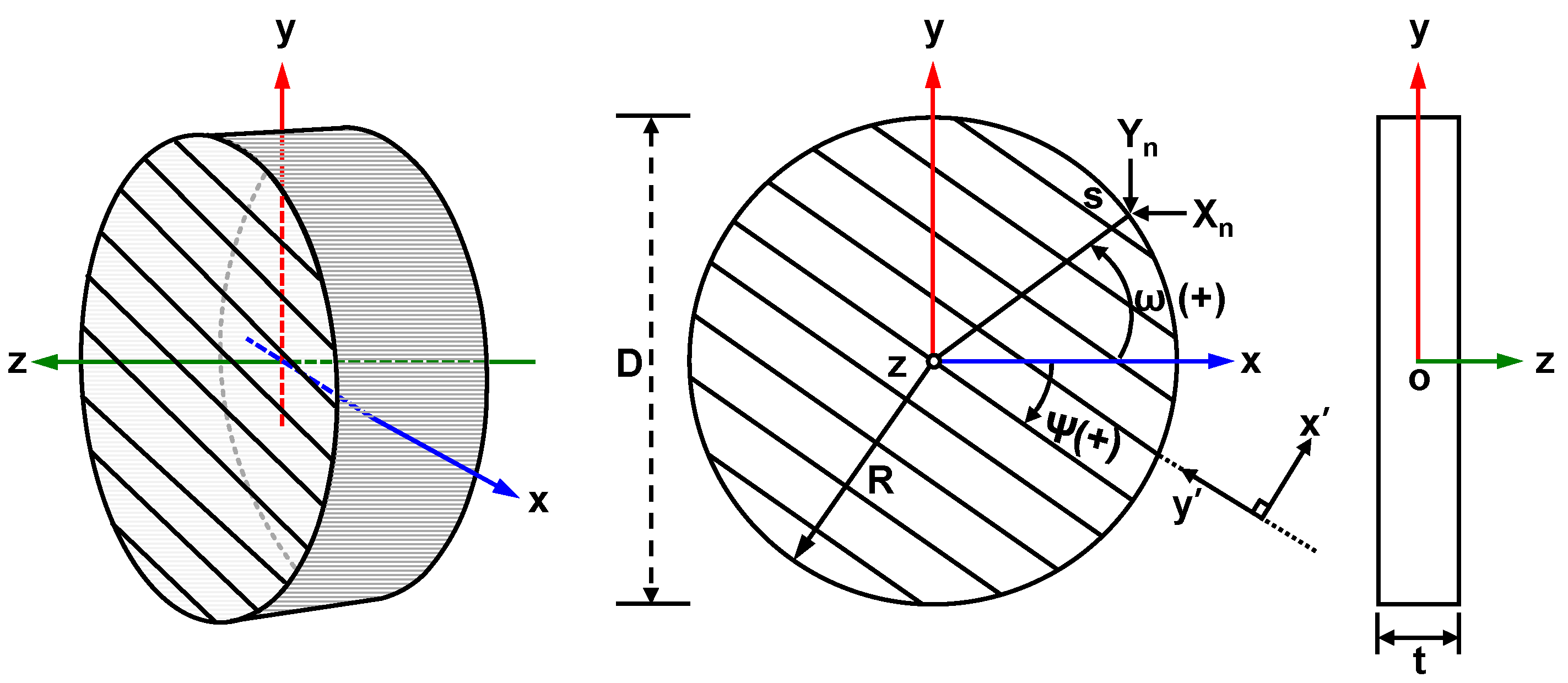
Figure 2.
Schematic drawing of a disc sample for loading in (a) the transversal isotropic plane and (b) in the plane perpendicular to the transversal isotropic plane.
Figure 2.
Schematic drawing of a disc sample for loading in (a) the transversal isotropic plane and (b) in the plane perpendicular to the transversal isotropic plane.
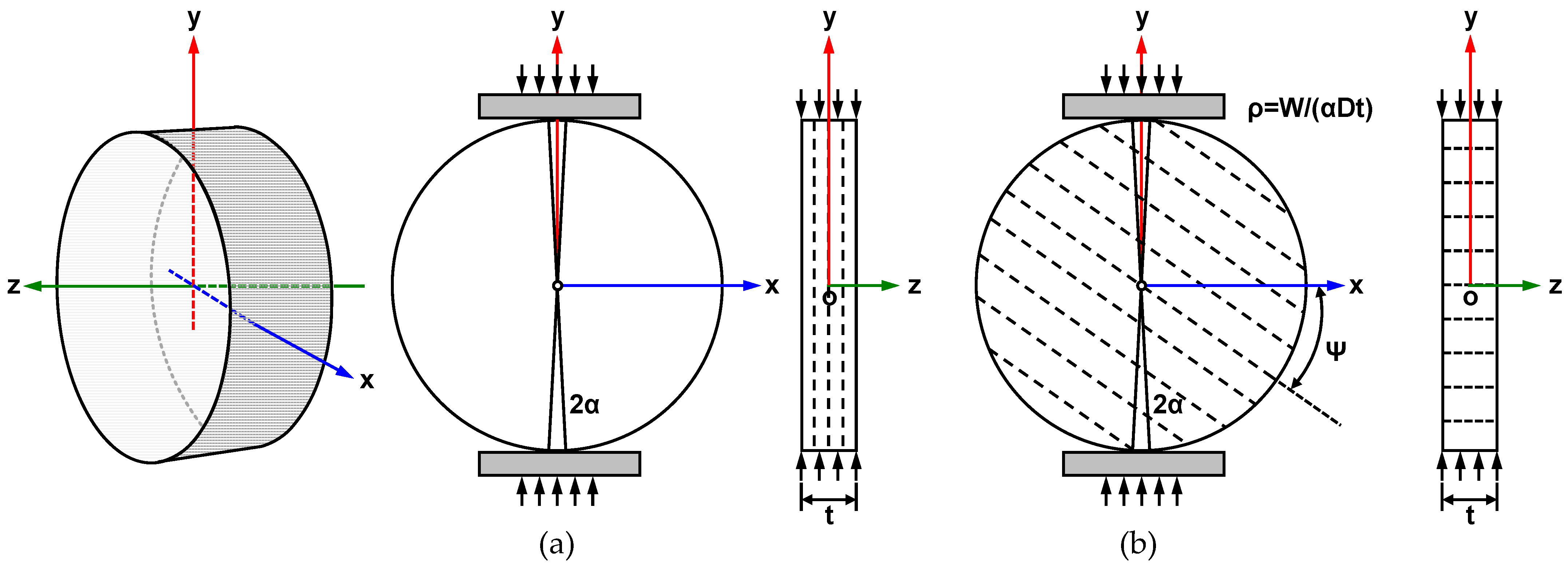
Figure 3.
Geological map of Daegu area indicating the black shale collection site.
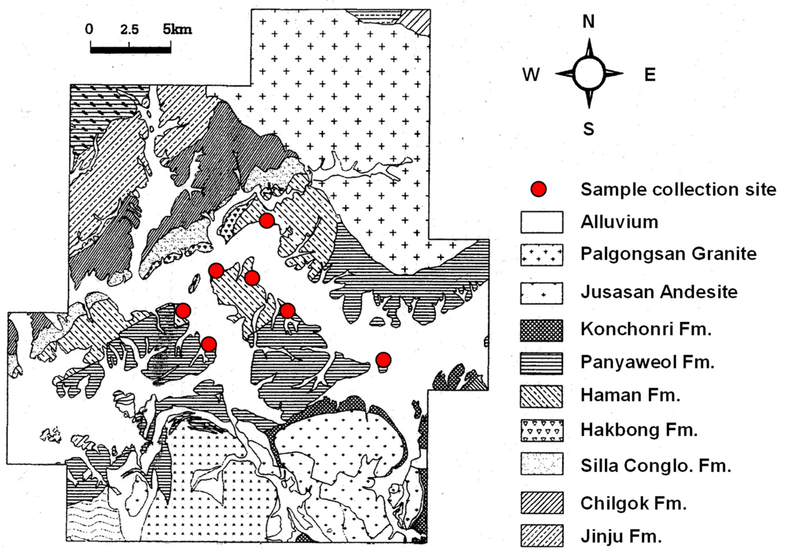
Figure 4.
(a) Results of the XRD test and (b) a photograph of SEM analysis of black shale.

Figure 5.
Black shale samples for uniaxial compression tests with angles of (a) θ = 0°, (b) θ = 90°, and (c) θ = 45°.
Figure 5.
Black shale samples for uniaxial compression tests with angles of (a) θ = 0°, (b) θ = 90°, and (c) θ = 45°.

Figure 6.
Black shale samples for Brazilian tests for (a) isotropy and diametric loading with the inclination angles of: (b) ψ = 0°, (c) ψ = 15°, (d) ψ = 30°, (e) ψ = 45°, (f) ψ = 60°, (g) ψ = 75°, and (h) ψ = 90°.
Figure 6.
Black shale samples for Brazilian tests for (a) isotropy and diametric loading with the inclination angles of: (b) ψ = 0°, (c) ψ = 15°, (d) ψ = 30°, (e) ψ = 45°, (f) ψ = 60°, (g) ψ = 75°, and (h) ψ = 90°.
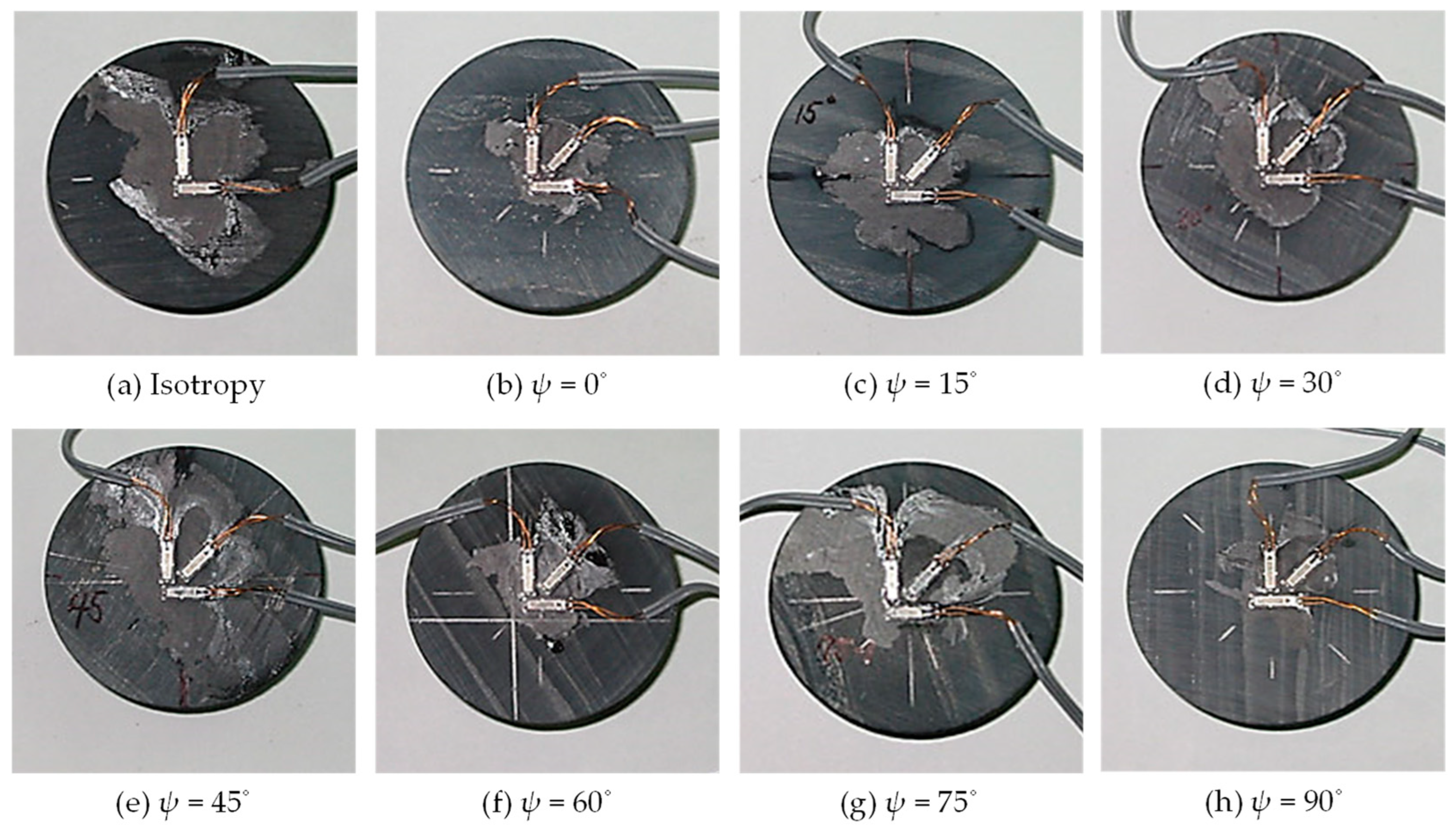
Figure 7.
Results of uniaxial compression test with angles of (a) θ = 0°, (b) θ = 45°, and (c) θ = 90°.
Figure 7.
Results of uniaxial compression test with angles of (a) θ = 0°, (b) θ = 45°, and (c) θ = 90°.

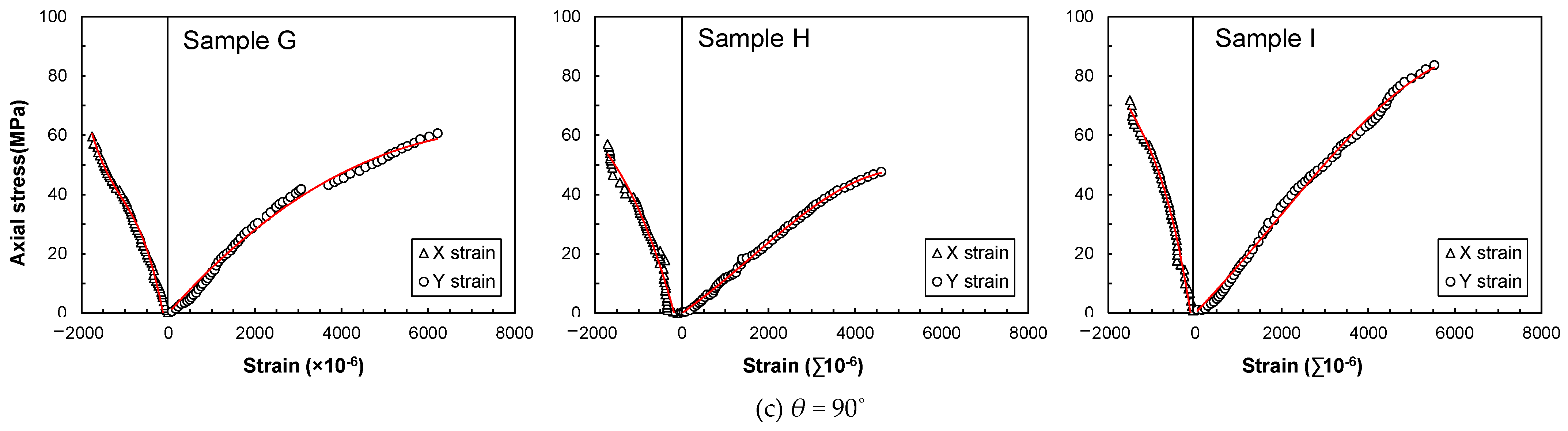
Figure 8.
Relationship between the unconfined compression strength and Young’s modulus (EY) for the black shale samples at different orientations (0°, 45°, and 90°).
Figure 8.
Relationship between the unconfined compression strength and Young’s modulus (EY) for the black shale samples at different orientations (0°, 45°, and 90°).

Figure 9.
Results of the Brazilian tests for (a) isotropy and diametral loading with inclination angles of (b) ψ = 0°, (c) ψ = 15°, (d) ψ = 30°, (e) ψ = 45°, (f) ψ = 60°, (g) ψ = 75°, and (h) ψ = 90°.
Figure 9.
Results of the Brazilian tests for (a) isotropy and diametral loading with inclination angles of (b) ψ = 0°, (c) ψ = 15°, (d) ψ = 30°, (e) ψ = 45°, (f) ψ = 60°, (g) ψ = 75°, and (h) ψ = 90°.
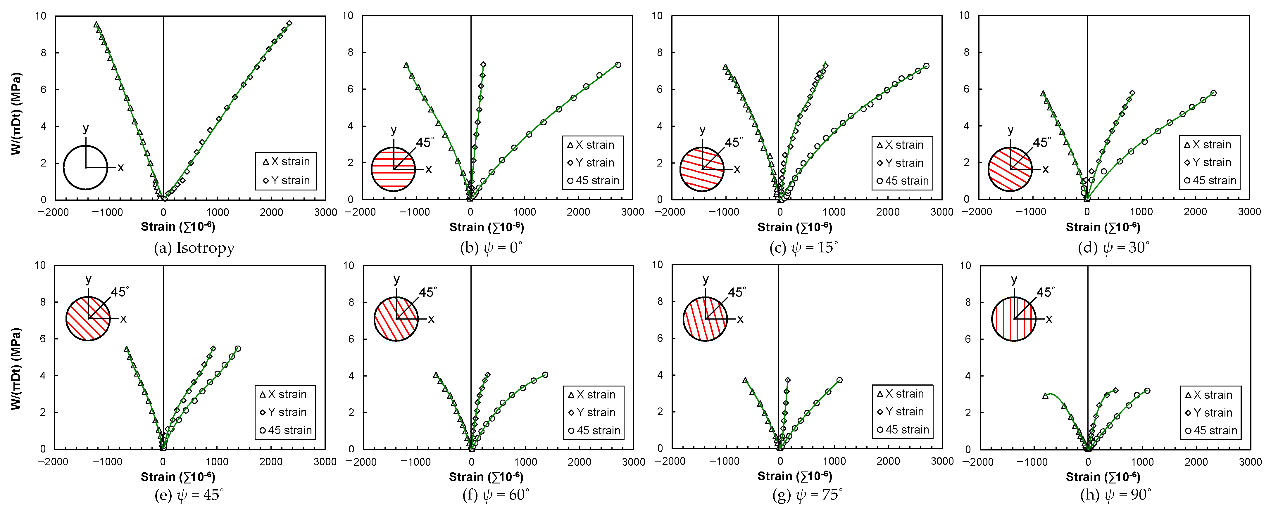
Figure 10.
Failure patterns of the sample for (a) isotropy and diametral loading with inclination angles of (b) ψ = 0°, (c) ψ = 15°, (d) ψ = 30°, (e) ψ = 45°, (f) ψ = 60°, (g) ψ = 75°, and (h) ψ = 90°.
Figure 10.
Failure patterns of the sample for (a) isotropy and diametral loading with inclination angles of (b) ψ = 0°, (c) ψ = 15°, (d) ψ = 30°, (e) ψ = 45°, (f) ψ = 60°, (g) ψ = 75°, and (h) ψ = 90°.

Figure 11.
Results of the elastic constants obtained from the Brazilian test with respect to the inclination angles (a) E′, (b) v′, and (c) G′.
Figure 11.
Results of the elastic constants obtained from the Brazilian test with respect to the inclination angles (a) E′, (b) v′, and (c) G′.

Figure 12.
Stress concentration coefficients with the half-loading strip angle.
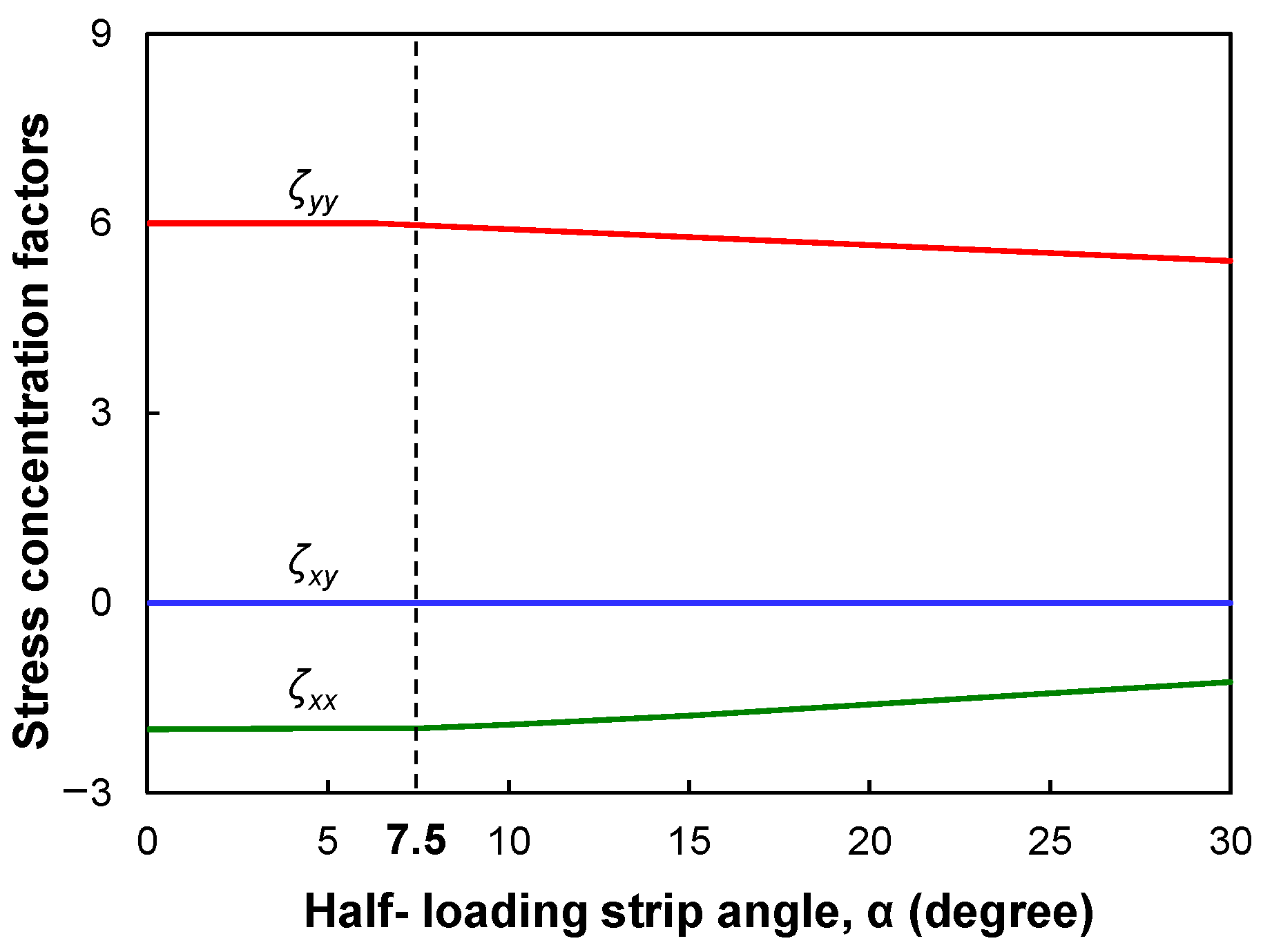
Figure 13.
Numerical results of the stress concentration coefficient for a transversely isotropic specimen: (a) ζxx, (b) ζyy, and (c) ζxy.
Figure 13.
Numerical results of the stress concentration coefficient for a transversely isotropic specimen: (a) ζxx, (b) ζyy, and (c) ζxy.
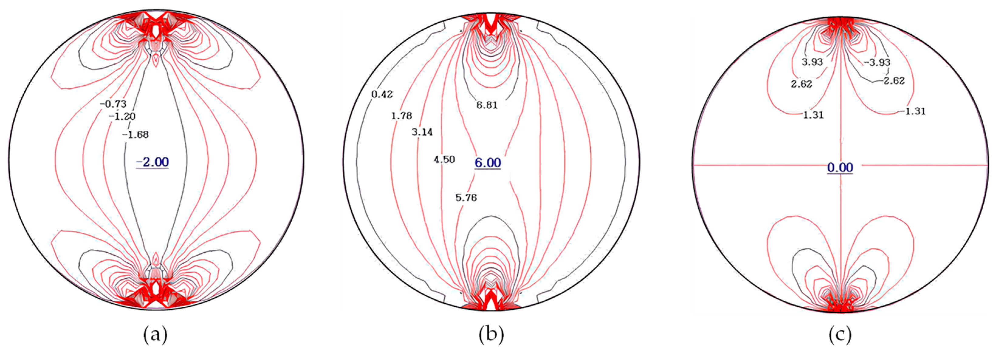
Figure 14.
Variation of the stress concentration coefficients with variation of the inclination angle: (a) ζxx, (b) ζyy, and (c) ζxy.
Figure 14.
Variation of the stress concentration coefficients with variation of the inclination angle: (a) ζxx, (b) ζyy, and (c) ζxy.
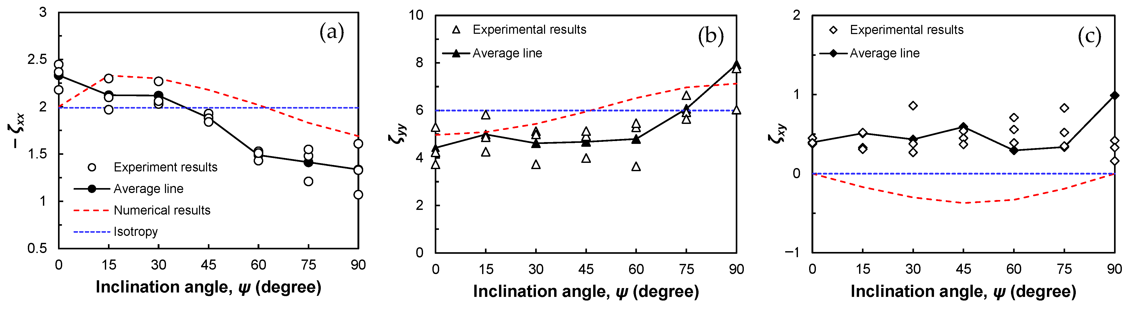
Figure 15.
Results of the indirect tensile strength.


Table 1.
Physical properties of black shale.
| Type | Sample No. | Natural State, Gn | Dry State, Gd | Saturated State, Gt | wn (%) | Sr (%) | ne (%) | ab (%) |
|---|---|---|---|---|---|---|---|---|
| Black shale | 1 | 2.743 | 2.739 | 2.746 | 0.16 | 59.57 | 0.75 | 0.27 |
| 2 | 2.742 | 2.724 | 2.745 | 0.65 | 72.65 | 2.13 | 0.78 | |
| 3 | 2.741 | 2.728 | 2.745 | 0.48 | 69.07 | 1.65 | 0.60 | |
| 4 | 2.742 | 2.736 | 2.745 | 0.20 | 62.22 | 0.89 | 0.33 | |
| 5 | 2.668 | 2.661 | 2.672 | 0.25 | 65.96 | 1.00 | 0.38 | |
| 6 | 2.674 | 2.647 | 2.680 | 0.30 | 79.65 | 3.34 | 0.26 | |
| 7 | 2.711 | 2.682 | 2.719 | 0.65 | 79.09 | 3.74 | 0.49 | |
| Average | 2.717 | 2.702 | 2.722 | 0.38 | 69.74 | 1.93 | 0.44 | |
Table 2.
Mineral composition of black shale.
| Sample | Component (%) | |||||||||
|---|---|---|---|---|---|---|---|---|---|---|
| Q | Or | Ab | An | Wo | Cm | Iim | Mt | Cc | Tn | |
| Black shale | 18.10 | 3.60 | 26.74 | - | - | 27.58 | 0.59 | 2.13 | 18.20 | 7.48 |
Table 3.
Uniaxial compression strengths and elastic constants obtained from the uniaxial compression test.
Table 3.
Uniaxial compression strengths and elastic constants obtained from the uniaxial compression test.
| Angle | Sample | Unconfined Compression Strength (MPa) | EY (GPa) | E (GPa) | ν | E′ (GPa) | ν′ | G (GPa) | G′ (GPa) |
|---|---|---|---|---|---|---|---|---|---|
| 0° | A | 89 | 14.16 | - | - | 14.16 | 0.21 | - | - |
| B | 86 | 15.44 | - | - | 15.44 | 0.14 | - | - | |
| C | 83 | 12.49 | - | - | 12.49 | 0.21 | - | - | |
| Average | 86 | 14.03 | - | - | 14.03 | 0.19 | - | - | |
| 45° | D | 60 | 14.53 | - | - | - | - | - | 10.63 |
| E | 57 | 11.69 | - | - | - | - | - | 8.09 | |
| F | 50 | 11.88 | - | - | - | - | - | 8.33 | |
| Average | 56 | 12.70 | - | - | - | - | - | 9.02 | |
| 90° | G | 75 | 27.25 | 30.77 | 0.27 | - | - | 11.24 | - |
| H | 69 | 28.89 | 33.30 | 0.24 | - | - | 12.64 | - | |
| I | 62 | 27.56 | 51.13 | 0.28 | - | - | 11.41 | - | |
| Average | 69 | 27.90 | 38.40 | 0.26 | - | - | 11.76 | - |
Table 4.
Strain measurements and determined elastic constants with the midplane parallel to the transversal isotropic plane.
Table 4.
Strain measurements and determined elastic constants with the midplane parallel to the transversal isotropic plane.
| Sample | D (mm) | t (mm) | εxπDt/W (MPa−1) | εyπDt/W (MPa−1) | E (GPa) | ν (-) | G (GPa) | Wf/πDt (MPa) |
|---|---|---|---|---|---|---|---|---|
| Isotropy | 54 | 26.5 | −1.18 | 2.27 | 4.97 | 0.533 | 1.62 | 9.61 |
Table 5.
Strain measurements and determined elastic constants with midplane perpendicular to the transversal isotropic plane.
Table 5.
Strain measurements and determined elastic constants with midplane perpendicular to the transversal isotropic plane.
| Sample | ψ (degree) | D (mm) | t (mm) | εxπDt/W (MPa−1) | ε45πDt/W (MPa−1) | εyπDt/W (MPa−1) | E′ (GPa) | ν′ (-) | G′ (GPa) | Wf/πDt (MPa) |
|---|---|---|---|---|---|---|---|---|---|---|
| A | 0° | 54 | 26.5 | −1.30 | 0.29 | 2.96 | 3.25 | 0.436 | 2.13 | 7.33 |
| 15° | 54 | 26.2 | −1.02 | 0.70 | 2.59 | 3.70 | 0.372 | 2.54 | 7.28 | |
| 30° | 54 | 24.2 | −1.14 | 1.04 | 3.17 | 3.22 | 0.348 | 2.24 | 5.77 | |
| 45° | 54 | 25.0 | −0.98 | 1.35 | 2.09 | 4.59 | 0.484 | 3.03 | 5.47 | |
| 60° | 54 | 27.2 | −1.20 | 0.41 | 2.09 | 4.60 | 0.481 | 2.62 | 4.06 | |
| 75° | 54 | 25.5 | −1.43 | 0.43 | 2.49 | 3.87 | 0.589 | 2.30 | 3.72 | |
| 90° | 54 | 26.1 | −1.59 | 0.60 | 2.76 | 3.22 | 0.730 | 1.98 | 3.21 |
Table 6.
Comparison of elastic constants derived from the uniaxial compression and indirect shear (Brazilian) tests.
Table 6.
Comparison of elastic constants derived from the uniaxial compression and indirect shear (Brazilian) tests.
| Test | E (GPa) | E′ (GPa) | ν (-) | ν′ (MPa) | G (GPa) | G′ (GPa) | E/E′ (-) | G/G′ (-) |
|---|---|---|---|---|---|---|---|---|
| Uniaxial comp. test | 38.40 | 14.03 | 0.260 | 0.190 | 11.76 | 9.02 | 2.737 | 1.304 |
| Brazilian test | 4.97 | 3.78 | 0.533 | 0.491 | 1.62 | 2.41 | 1.315 | 0.672 |
Table 7.
Results of the stress concentration coefficients using experimental and numerical methods.
| Inclination Angle, ψ | Sample | Failure Stress (MPa) | Stress Concentration Coefficients | |||||
|---|---|---|---|---|---|---|---|---|
| Experimental Method | Numerical Method | |||||||
| ζ xx | ζ yy | ζ xy | ζ xx | ζ yy | ζ xy | |||
| Isotropy | A | 9.60 | −1.99 | - | - | −2.00 | 6.00 | 0.00 |
| B | 9.11 | −2.02 | - | - | ||||
| C | 9.15 | −1.96 | - | - | ||||
| Average | 9.30 | −1.99 | - | - | ||||
| 0° | A | 7.32 | −2.45 | 3.73 | 0.27 | −2.33 | 4.97 | 0.00 |
| B | 8.85 | −2.37 | 4.24 | 0.38 | ||||
| C | 5.58 | −2.18 | 5.30 | 0.54 | ||||
| Average | 7.25 | −2.33 | 4.42 | 0.40 | ||||
| 15° | A | 6.36 | −1.97 | 5.83 | 0.45 | −2.30 | 5.09 | −0.17 |
| B | 7.69 | −2.30 | 4.26 | 0.37 | ||||
| C | 6.44 | −2.10 | 4.87 | 0.71 | ||||
| Average | 6.83 | −2.12 | 4.99 | 0.51 | ||||
| 30° | A | 5.76 | −2.03 | 5.12 | 0.39 | −2.18 | 5.43 | −0.30 |
| B | 4.37 | −2.06 | 3.73 | 0.56 | ||||
| C | 4.75 | −2.27 | 4.99 | 0.35 | ||||
| Average | 4.96 | −2.12 | 4.61 | 0.43 | ||||
| 45° | A | 5.45 | −1.93 | 3.99 | 0.83 | −2.02 | 5.95 | −0.37 |
| B | 6.26 | −1.88 | 4.92 | 0.52 | ||||
| C | 4.57 | −1.84 | 5.13 | 0.42 | ||||
| Average | 5.42 | −1.88 | 4.68 | 0.59 | ||||
| 60° | A | 4.05 | −1.53 | 5.29 | 0.16 | −1.83 | 6.52 | −0.33 |
| B | 6.26 | −1.34 | 5.46 | 0.33 | ||||
| C | 4.71 | −1.51 | 3.65 | 0.39 | ||||
| Average | 5.01 | −1.46 | 4.8 | 0.29 | ||||
| 75° | A | 3.70 | −1.21 | 6.64 | 0.31 | −1.69 | 6.97 | −0.19 |
| B | 4.26 | −1.48 | 5.92 | 0.18 | ||||
| C | 4.08 | −1.55 | 5.64 | 0.52 | ||||
| Average | 4.02 | −1.41 | 6.07 | 0.34 | ||||
| 90° | A | 3.20 | −1.33 | 7.77 | 0.73 | −1.64 | 7.13 | 0.00 |
| B | 2.29 | −1.07 | 10.01 | 0.86 | ||||
| C | 2.10 | −1.61 | 6.03 | 1.38 | ||||
| Average | 2.53 | −1.34 | 7.94 | 0.99 | ||||
Disclaimer/Publisher’s Note: The statements, opinions and data contained in all publications are solely those of the individual author(s) and contributor(s) and not of MDPI and/or the editor(s). MDPI and/or the editor(s) disclaim responsibility for any injury to people or property resulting from any ideas, methods, instructions or products referred to in the content. |
© 2024 by the author. Licensee MDPI, Basel, Switzerland. This article is an open access article distributed under the terms and conditions of the Creative Commons Attribution (CC BY) license (https://creativecommons.org/licenses/by/4.0/).
Share and Cite
MDPI and ACS Style
Kim, M. Investigation of Indirect Shear Strength of Black Shale for Urban Deep Excavation. Buildings 2024, 14, 3050. https://doi.org/10.3390/buildings14103050
AMA Style
Kim M. Investigation of Indirect Shear Strength of Black Shale for Urban Deep Excavation. Buildings. 2024; 14(10):3050. https://doi.org/10.3390/buildings14103050
Chicago/Turabian StyleKim, Mintae. 2024. "Investigation of Indirect Shear Strength of Black Shale for Urban Deep Excavation" Buildings 14, no. 10: 3050. https://doi.org/10.3390/buildings14103050
Note that from the first issue of 2016, this journal uses article numbers instead of page numbers. See further details here.