

Relationship between CO2 Emissions from Concrete Production and Economic Growth in 20 OECD Countries

Abstract
:1. Introduction
2. Research Background
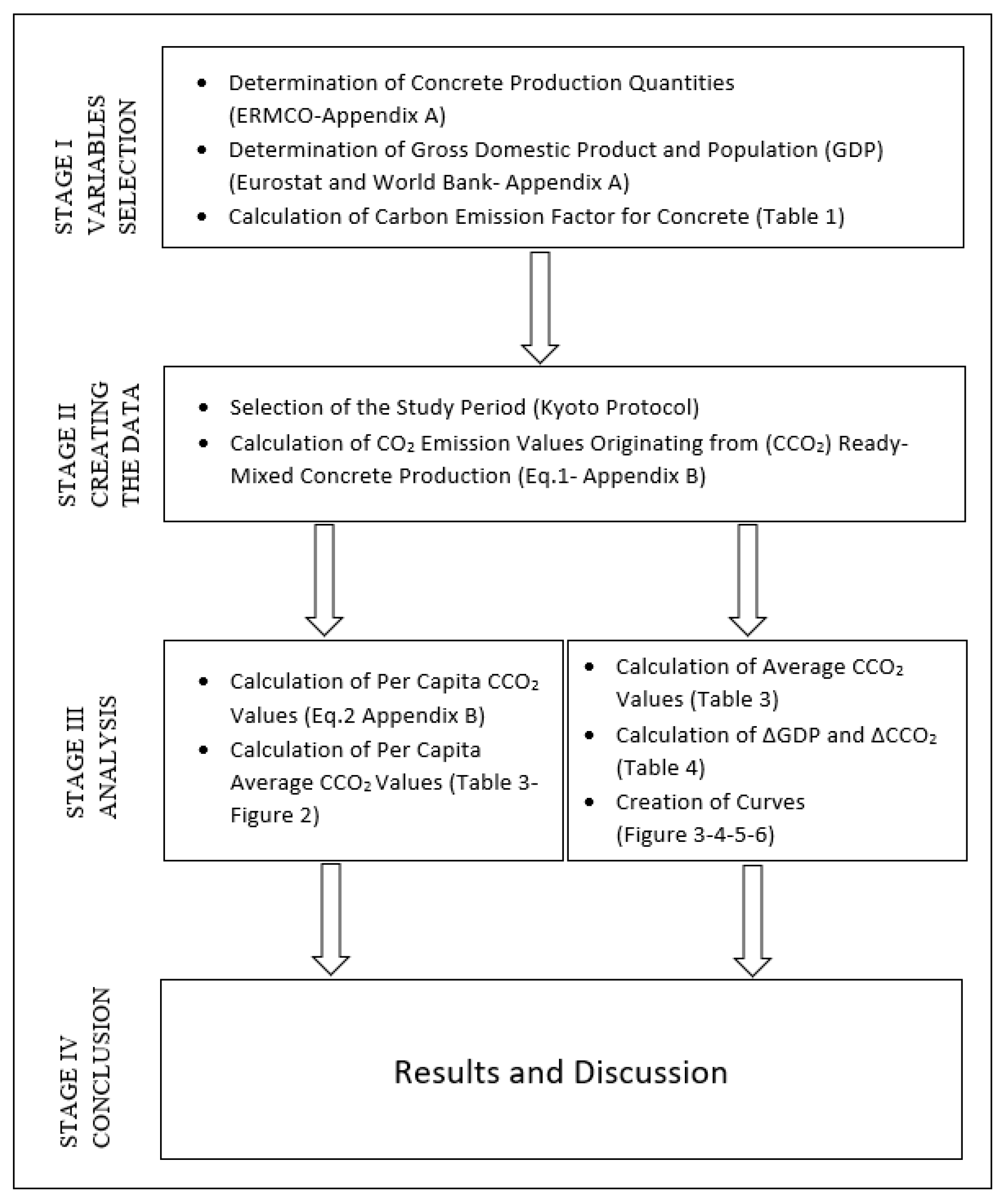
3. Research Methodology
4. Data Analysis and Findings
5. Discussion
6. Conclusions
Funding
Data Availability Statement
Conflicts of Interest
Appendix A

| Country | 2000 | 2001 | 2002 | 2003 | 2004 | 2005 | 2006 | 2007 | 2008 | 2009 | 2010 | 2011 | 2012 | 2013 | 2014 | 2015 | 2016 | 2017 | 2018 | 2019 | Av. | |
|---|---|---|---|---|---|---|---|---|---|---|---|---|---|---|---|---|---|---|---|---|---|---|
| AUS | RMC | 9.30 | 7.30 | 9.60 | 10.00 | 9.90 | 11.00 | 11.00 | 11.30 | 11.50 | 10.30 | 10.20 | 10.50 | 10.60 | 10.50 | 10.00 | 10.50 | 10.80 | 11.00 | 11.80 | 11.90 | 10.45 |
| GDP | 197.29 | 197.51 | 214.39 | 262.27 | 301.46 | 316.09 | 336.28 | 389.19 | 432.05 | 401.76 | 392.28 | 431.69 | 409.40 | 430.19 | 442.58 | 381.97 | 395.84 | 417.26 | 454.99 | 444.60 | 362.45 | |
| P | 8.01 | 8.04 | 8.08 | 8.12 | 8.17 | 8.23 | 8.27 | 8.30 | 8.32 | 8.34 | 8.36 | 8.39 | 8.43 | 8.48 | 8.55 | 8.64 | 8.74 | 8.80 | 8.84 | 8.88 | 8.40 | |
| BEL | RMC | 11.80 | 10.90 | 9.90 | 10.80 | 11.20 | 11.00 | 12.20 | 12.00 | 11.80 | 10.40 | 10.80 | 11.60 | 12.50 | 13.00 | 12.30 | 12.30 | 12.50 | 12.70 | 12.80 | 13.00 | 11.78 |
| GDP | 236.79 | 236.75 | 258.38 | 318.08 | 369.21 | 385.71 | 408.26 | 470.92 | 517.33 | 483.25 | 481.42 | 523.33 | 496.15 | 521.79 | 535.39 | 462.34 | 476.06 | 502.76 | 543.30 | 535.87 | 438.16 | |
| P | 10.25 | 10.29 | 10.33 | 10.38 | 10.42 | 10.48 | 10.55 | 10.63 | 10.71 | 10.80 | 10.90 | 11.04 | 11.11 | 11.16 | 11.21 | 11.27 | 11.33 | 11.38 | 11.43 | 11.49 | 10.86 | |
| CZE | RMC | 5.50 | 5.50 | 5.50 | 6.00 | 6.40 | 7.40 | 8.00 | 8.50 | 9.60 | 7.30 | 6.40 | 7.50 | 6.90 | 6.50 | 6.50 | 6.50 | 6.80 | 6.80 | 7.10 | 7.10 | 6.89 |
| GDP | 61.83 | 67.81 | 82.20 | 100.09 | 119.81 | 137.14 | 156.26 | 190.18 | 236.82 | 207.43 | 209.07 | 229.56 | 208.86 | 211.69 | 209.36 | 188.03 | 196.27 | 218.63 | 249.00 | 252.55 | 176.63 | |
| P | 10.26 | 10.22 | 10.20 | 10.19 | 10.20 | 10.21 | 10.24 | 10.30 | 10.38 | 10.44 | 10.47 | 10.50 | 10.51 | 10.51 | 10.53 | 10.55 | 10.57 | 10.59 | 10.63 | 10.67 | 10.41 | |
| DEN | RMC | 2.20 | 2.10 | 2.30 | 2.20 | 2.30 | 2.60 | 2.80 | 2.90 | 2.70 | 1.80 | 1.70 | 2.10 | 2.00 | 2.30 | 2.30 | 2.50 | 2.50 | 2.60 | 2.60 | 2.70 | 2.36 |
| GDP | 164.16 | 164.79 | 178.64 | 218.10 | 251.37 | 264.47 | 282.88 | 319.42 | 353.36 | 321.24 | 322.00 | 344.00 | 327.15 | 343.58 | 352.99 | 302.67 | 313.12 | 332.12 | 356.84 | 346.50 | 292.97 | |
| P | 5.34 | 5.36 | 5.38 | 5.39 | 5.40 | 5.42 | 5.44 | 5.46 | 5.49 | 5.52 | 5.55 | 5.57 | 5.59 | 5.61 | 5.64 | 5.68 | 5.73 | 5.76 | 5.79 | 5.81 | 5.55 | |
| FIN | RMC | 2.50 | 2.60 | 2.60 | 2.30 | 2.40 | 2.50 | 2.70 | 3.10 | 2.80 | 2.00 | 2.60 | 3.00 | 2.70 | 2.70 | 2.60 | 2.60 | 2.90 | 3.00 | 2.80 | 2.70 | 2.66 |
| GDP | 126.02 | 129.53 | 140.40 | 171.65 | 197.48 | 204.89 | 217.09 | 256.38 | 285.72 | 253.50 | 249.42 | 275.60 | 258.29 | 271.36 | 274.86 | 234.53 | 240.77 | 255.65 | 275.71 | 268.51 | 229.37 | |
| P | 5.18 | 5.19 | 5.20 | 5.21 | 5.23 | 5.25 | 5.27 | 5.29 | 5.31 | 5.34 | 5.36 | 5.39 | 5.41 | 5.44 | 5.46 | 5.48 | 5.50 | 5.51 | 5.52 | 5.52 | 5.35 | |
| FRA | RMC | 34.30 | 34.50 | 34.60 | 34.80 | 37.50 | 40.50 | 43.40 | 45.00 | 44.20 | 37.00 | 37.40 | 41.30 | 38.90 | 38.60 | 36.40 | 34.80 | 36.10 | 38.60 | 39.70 | 40.30 | 38.40 |
| GDP | 1365.64 | 1377.66 | 1501.41 | 1844.54 | 2119.63 | 2196.95 | 2320.54 | 2660.59 | 2930.30 | 2700.89 | 2645.19 | 2865.16 | 2683.67 | 2811.88 | 2855.96 | 2439.19 | 2472.96 | 2595.15 | 2790.96 | 2728.87 | 2395.36 | |
| P | 60.92 | 61.37 | 61.82 | 62.26 | 62.72 | 63.19 | 63.63 | 64.02 | 64.38 | 64.71 | 65.03 | 65.35 | 65.66 | 66.00 | 66.31 | 66.55 | 66.72 | 66.92 | 67.16 | 67.39 | 64.60 | |
| GER | RMC | 57.90 | 51.10 | 46.90 | 47.20 | 44.20 | 18.00 | 24.00 | 40.80 | 41.00 | 37.70 | 42.00 | 48.00 | 46.00 | 45.60 | 46.80 | 46.00 | 49.50 | 52.00 | 52.70 | 53.50 | 44.55 |
| GDP | 1947.98 | 1945.79 | 2078.48 | 2501.64 | 2814.35 | 2846.86 | 2994.70 | 3425.58 | 3745.26 | 3411.26 | 3399.67 | 3749.31 | 3527.14 | 3733.80 | 3889.09 | 3357.59 | 3469.85 | 3690.85 | 3974.44 | 3889.18 | 3219.64 | |
| P | 82.21 | 82.35 | 82.49 | 82.53 | 82.52 | 82.47 | 82.38 | 82.27 | 82.11 | 81.90 | 81.78 | 80.27 | 80.43 | 80.65 | 80.98 | 81.69 | 82.35 | 82.66 | 82.91 | 83.09 | 82.00 | |
| IRE | RMC | 5.90 | 6.00 | 7.50 | 7.50 | 8.50 | 10.00 | 9.20 | 9.00 | 10.00 | 3.80 | 2.70 | 2.40 | 2.10 | 2.10 | 2.40 | 2.40 | 4.20 | 4.30 | 4.30 | 4.30 | 5.43 |
| GDP | 100.21 | 109.35 | 128.60 | 164.67 | 194.37 | 211.88 | 232.18 | 270.08 | 275.45 | 236.44 | 221.91 | 239.17 | 225.12 | 238.11 | 259.68 | 292.36 | 298.56 | 337.24 | 386.69 | 398.93 | 241.05 | |
| P | 3.81 | 3.87 | 3.93 | 4.00 | 4.07 | 4.16 | 4.27 | 4.40 | 4.49 | 4.54 | 4.56 | 4.58 | 4.60 | 4.62 | 4.66 | 4.70 | 4.76 | 4.81 | 4.87 | 4.93 | 4.43 | |
| ITA | RMC | 66.50 | 66.80 | 71.50 | 72.80 | 72.80 | 77.40 | 77.50 | 75.20 | 73.20 | 56.30 | 53.20 | 52.60 | 39.90 | 31.70 | 28.00 | 25.30 | 27.40 | 27.30 | 27.30 | 28.40 | 52.56 |
| GDP | 1146.68 | 1168.02 | 1276.77 | 1577.62 | 1806.54 | 1858.22 | 1949.55 | 2213.10 | 2408.66 | 2199.93 | 2136.10 | 2294.99 | 2086.96 | 2141.92 | 2162.01 | 1836.64 | 1877.07 | 1961.80 | 2091.93 | 2011.30 | 1910.29 | |
| P | 56.94 | 56.97 | 57.06 | 57.31 | 57.69 | 57.97 | 58.14 | 58.44 | 58.83 | 59.10 | 59.28 | 59.38 | 59.54 | 60.23 | 60.79 | 60.73 | 60.63 | 60.54 | 60.42 | 59.73 | 58.99 | |
| NET | RMC | 8.50 | 8.50 | 8.10 | 8.30 | 7.80 | 8.60 | 8.50 | 8.90 | 10.50 | 9.30 | 8.10 | 8.80 | 7.30 | 6.60 | 6.50 | 6.30 | 6.50 | 6.90 | 7.50 | 7.80 | 7.97 |
| GDP | 417.48 | 431.59 | 473.86 | 580.07 | 658.38 | 685.35 | 733.96 | 848.56 | 951.87 | 871.52 | 847.38 | 905.27 | 838.92 | 877.17 | 892.17 | 765.57 | 784.06 | 833.87 | 914.04 | 910.19 | 761.06 | |
| P | 15.93 | 16.05 | 16.15 | 16.23 | 16.28 | 16.32 | 16.35 | 16.38 | 16.45 | 16.53 | 16.62 | 16.69 | 16.75 | 16.80 | 16.87 | 16.94 | 17.03 | 17.13 | 17.23 | 17.34 | 16.60 | |
| POL | RMC | 10.00 | 9.00 | 8.70 | 8.90 | 10.50 | 11.00 | 14.20 | 16.00 | 21.20 | 17.70 | 18.60 | 23.70 | 19.50 | 18.00 | 19.20 | 19.80 | 20.40 | 20.40 | 25.10 | 26.20 | 16.91 |
| GDP | 172.22 | 190.91 | 199.07 | 217.83 | 255.11 | 306.15 | 344.63 | 429.02 | 533.60 | 439.73 | 475.70 | 524.37 | 495.23 | 515.76 | 539.08 | 477.11 | 470.02 | 524.64 | 588.78 | 596.06 | 414.75 | |
| P | 38.26 | 38.25 | 38.23 | 38.20 | 38.18 | 38.17 | 38.14 | 38.12 | 38.13 | 38.15 | 38.04 | 38.06 | 38.06 | 38.04 | 38.01 | 37.99 | 37.97 | 37.97 | 37.97 | 37.97 | 38.10 | |
| POR | RMC | 10.00 | 11.30 | 10.50 | 9.50 | 11.50 | 12.00 | 11.00 | 11.50 | 11.00 | 8.50 | 7.50 | 6.10 | 3.70 | 2.70 | 2.80 | 2.80 | 3.20 | 3.70 | 4.50 | 5.10 | 7.45 |
| GDP | 118.61 | 121.60 | 134.80 | 165.23 | 189.38 | 197.25 | 208.76 | 240.50 | 263.42 | 244.67 | 238.11 | 245.12 | 216.22 | 226.43 | 229.90 | 199.39 | 206.43 | 221.36 | 242.31 | 239.99 | 207.47 | |
| P | 10.29 | 10.36 | 10.42 | 10.46 | 10.48 | 10.50 | 10.52 | 10.54 | 10.56 | 10.57 | 10.57 | 10.56 | 10.51 | 10.46 | 10.40 | 10.36 | 10.33 | 10.30 | 10.28 | 10.29 | 10.44 | |
| SLO | RMC | 1.90 | 1.90 | 1.90 | 2.10 | 2.40 | 2.70 | 2.90 | 3.20 | 3.70 | 2.60 | 2.40 | 2.30 | 1.90 | 1.70 | 1.60 | 1.90 | 1.90 | 2.40 | 3.00 | 2.80 | 2.36 |
| GDP | 29.24 | 30.78 | 35.30 | 46.92 | 57.44 | 62.81 | 70.77 | 86.56 | 100.88 | 89.40 | 91.16 | 99.92 | 94.62 | 98.94 | 101.44 | 88.90 | 89.95 | 95.65 | 106.14 | 105.71 | 79.13 | |
| P | 5.39 | 5.38 | 5.38 | 5.37 | 5.37 | 5.37 | 5.37 | 5.37 | 5.38 | 5.39 | 5.39 | 5.40 | 5.41 | 5.41 | 5.42 | 5.42 | 5.43 | 5.44 | 5.45 | 5.45 | 5.40 | |
| SPA | RMC | 64.00 | 71.10 | 73.50 | 81.00 | 82.00 | 87.60 | 97.80 | 95.30 | 69.00 | 49.00 | 39.10 | 30.80 | 21.60 | 16.30 | 15.90 | 16.30 | 16.30 | 19.70 | 22.20 | 24.80 | 49.67 |
| GDP | 598.36 | 627.83 | 708.76 | 907.49 | 1069.06 | 1153.72 | 1260.40 | 1474.00 | 1631.86 | 1491.47 | 1422.11 | 1480.71 | 1324.75 | 1355.58 | 1371.82 | 1196.16 | 1233.55 | 1313.25 | 1421.70 | 1394.32 | 1221.85 | |
| P | 40.57 | 40.85 | 41.43 | 42.19 | 42.92 | 43.65 | 44.40 | 45.23 | 45.95 | 46.36 | 46.58 | 46.74 | 46.77 | 46.62 | 46.48 | 46.44 | 46.48 | 46.59 | 46.80 | 47.13 | 45.01 | |
| SWE | RMC | 2.40 | 2.60 | 2.40 | 2.40 | 2.50 | 2.70 | 3.00 | 3.30 | 3.50 | 2.80 | 3.30 | 3.30 | 3.30 | 3.30 | 3.30 | 3.30 | 4.50 | 4.50 | 4.50 | 4.50 | 3.27 |
| GDP | 262.84 | 242.40 | 266.85 | 334.34 | 385.12 | 392.22 | 423.09 | 491.25 | 517.71 | 436.54 | 495.81 | 574.09 | 552.48 | 586.84 | 581.96 | 505.10 | 515.65 | 541.02 | 555.46 | 533.88 | 459.73 | |
| P | 8.87 | 8.90 | 8.92 | 8.96 | 8.99 | 9.03 | 9.08 | 9.15 | 9.22 | 9.30 | 9.38 | 9.45 | 9.52 | 9.60 | 9.70 | 9.80 | 9.92 | 10.06 | 10.18 | 10.28 | 9.41 | |
| UK | RMC | 23.00 | 23.00 | 23.00 | 25.00 | 25.00 | 25.20 | 25.10 | 25.60 | 20.50 | 15.80 | 15.70 | 19.20 | 17.60 | 19.60 | 22.70 | 23.70 | 24.60 | 22.90 | 25.70 | 24.90 | 22.39 |
| GDP | 1665.53 | 1649.83 | 1785.73 | 2054.42 | 2421.53 | 2543.18 | 2708.44 | 3090.51 | 2929.41 | 2412.84 | 2485.48 | 2663.81 | 2707.09 | 2784.85 | 3064.71 | 2927.91 | 2689.11 | 2680.15 | 2871.34 | 2851.41 | 2549.36 | |
| P | 58.89 | 59.12 | 59.37 | 59.65 | 59.99 | 60.40 | 60.85 | 61.32 | 61.81 | 62.28 | 62.77 | 63.26 | 63.70 | 64.13 | 64.60 | 65.12 | 65.61 | 66.06 | 66.46 | 66.84 | 62.61 | |
| NOR | RMC | 2.30 | 2.20 | 2.20 | 2.30 | 2.70 | 3.10 | 3.20 | 3.80 | 3.70 | 2.90 | 3.00 | 3.50 | 3.70 | 3.80 | 3.80 | 3.70 | 4.00 | 4.10 | 4.10 | 3.80 | 3.30 |
| GDP | 171.46 | 174.24 | 195.91 | 229.39 | 265.27 | 309.98 | 346.92 | 402.64 | 464.92 | 387.98 | 431.05 | 501.36 | 512.78 | 526.01 | 501.74 | 388.16 | 370.96 | 401.75 | 439.79 | 408.74 | 371.55 | |
| P | 4.49 | 4.51 | 4.54 | 4.56 | 4.59 | 4.62 | 4.66 | 4.71 | 4.77 | 4.83 | 4.89 | 4.95 | 5.02 | 5.08 | 5.14 | 5.19 | 5.23 | 5.28 | 5.31 | 5.35 | 4.89 | |
| SWI | RMC | 10.50 | 10.90 | 10.00 | 9.30 | 9.80 | 11.10 | 12.10 | 12.10 | 12.10 | 12.10 | 12.10 | 12.50 | 13.00 | 12.00 | 12.00 | 12.00 | 11.50 | 11.50 | 10.90 | 11.10 | 11.43 |
| GDP | 279.22 | 286.58 | 309.30 | 362.08 | 403.91 | 418.28 | 441.63 | 490.74 | 567.27 | 554.21 | 598.85 | 715.89 | 686.42 | 706.23 | 726.54 | 694.12 | 687.90 | 695.20 | 725.57 | 721.37 | 553.57 | |
| P | 7.18 | 7.23 | 7.28 | 7.34 | 7.39 | 7.44 | 7.48 | 7.55 | 7.65 | 7.74 | 7.82 | 7.91 | 8.00 | 8.09 | 8.19 | 8.28 | 8.37 | 8.45 | 8.51 | 8.58 | 7.83 | |
| TUR | RMC | 27.00 | 25.40 | 26.80 | 28.20 | 37.10 | 46.30 | 70.70 | 74.40 | 69.60 | 66.40 | 79.70 | 90.00 | 93.00 | 102.00 | 107.00 | 107.00 | 109.00 | 115.00 | 100.00 | 67.00 | 72.08 |
| GDP | 274.29 | 201.75 | 240.25 | 314.60 | 408.87 | 506.31 | 557.08 | 681.32 | 770.45 | 649.29 | 776.97 | 838.79 | 880.56 | 957.80 | 938.93 | 864.31 | 869.68 | 858.99 | 778.97 | 761.01 | 656.51 | |
| P | 64.11 | 65.07 | 65.99 | 66.87 | 67.79 | 68.70 | 69.60 | 70.16 | 71.05 | 72.04 | 73.14 | 74.22 | 75.18 | 76.15 | 77.18 | 78.22 | 79.28 | 80.31 | 81.41 | 82.58 | 72.95 | |
| USA | RMC | 315.00 | 315.00 | 300.00 | 310.00 | 330.00 | 345.00 | 330.00 | 315.00 | 270.00 | 243.00 | 243.00 | 203.00 | 225.00 | 230.00 | 230.00 | 260.00 | 65.00 | 270.00 | 274.00 | 280.00 | 267.65 |
| GDP | 10,250.9 | 10,581.9 | 10,929.1 | 11,456.4 | 12,217.1 | 13,039.2 | 13,815.6 | 14,474.2 | 14,769.9 | 14,478.1 | 15,048.9 | 15,599.7 | 16,253.9 | 16,843.2 | 17,550.7 | 18,206.0 | 18,695.1 | 19,477.3 | 20,533.1 | 21,380.9 | 15,280.1 | |
| P | 282.16 | 284.97 | 287.63 | 290.11 | 292.81 | 295.52 | 298.38 | 301.23 | 304.09 | 306.77 | 309.33 | 311.58 | 313.88 | 316.06 | 318.39 | 320.74 | 323.07 | 325.12 | 326.84 | 328.33 | 306.85 |
Appendix B
| Country | 2000 | 2001 | 2002 | 2003 | 2004 | 2005 | 2006 | 2007 | 2008 | 2009 | 2010 | 2011 | 2012 | 2013 | 2014 | 2015 | 2016 | 2017 | 2018 | 2019 | Av. | |
|---|---|---|---|---|---|---|---|---|---|---|---|---|---|---|---|---|---|---|---|---|---|---|
| AUS | CCO2 | 2.80 | 2.20 | 2.89 | 3.01 | 2.98 | 3.31 | 3.31 | 3.40 | 3.46 | 3.10 | 3.07 | 3.16 | 3.19 | 3.16 | 3.01 | 3.16 | 3.25 | 3.31 | 3.55 | 3.58 | 3.15 |
| CCO2 per capita | 0.35 | 0.27 | 0.36 | 0.37 | 0.36 | 0.40 | 0.40 | 0.41 | 0.42 | 0.37 | 0.37 | 0.38 | 0.38 | 0.37 | 0.35 | 0.37 | 0.37 | 0.38 | 0.40 | 0.40 | 0.37 | |
| BEL | CCO2 | 3.55 | 3.28 | 2.98 | 3.25 | 3.37 | 3.31 | 3.68 | 3.61 | 3.55 | 3.13 | 3.25 | 3.49 | 3.77 | 3.92 | 3.71 | 3.71 | 3.77 | 3.83 | 3.86 | 3.92 | 3.55 |
| CCO2 per capita | 0.35 | 0.32 | 0.29 | 0.31 | 0.32 | 0.32 | 0.35 | 0.34 | 0.33 | 0.29 | 0.30 | 0.32 | 0.34 | 0.35 | 0.33 | 0.33 | 0.33 | 0.34 | 0.34 | 0.34 | 0.33 | |
| CZE | CCO2 | 1.66 | 1.66 | 1.66 | 1.81 | 1.93 | 2.23 | 2.41 | 2.56 | 2.89 | 2.20 | 1.93 | 2.26 | 2.08 | 1.96 | 1.96 | 1.96 | 2.05 | 2.05 | 2.14 | 2.14 | 2.08 |
| CCO2 per capita | 0.16 | 0.16 | 0.16 | 0.18 | 0.19 | 0.22 | 0.24 | 0.25 | 0.28 | 0.21 | 0.18 | 0.22 | 0.20 | 0.19 | 0.19 | 0.19 | 0.19 | 0.19 | 0.20 | 0.20 | 0.20 | |
| DEN | CCO2 | 0.66 | 0.63 | 0.69 | 0.66 | 0.69 | 0.78 | 0.84 | 0.87 | 0.81 | 0.54 | 0.51 | 0.63 | 0.60 | 0.69 | 0.69 | 0.75 | 0.75 | 0.78 | 0.78 | 0.81 | 0.71 |
| CCO2 per capita | 0.12 | 0.12 | 0.13 | 0.12 | 0.13 | 0.14 | 0.16 | 0.16 | 0.15 | 0.10 | 0.09 | 0.11 | 0.11 | 0.12 | 0.12 | 0.13 | 0.13 | 0.14 | 0.14 | 0.14 | 0.13 | |
| FIN | CCO2 | 0.75 | 0.78 | 0.78 | 0.69 | 0.72 | 0.75 | 0.81 | 0.93 | 0.84 | 0.60 | 0.78 | 0.90 | 0.81 | 0.81 | 0.78 | 0.78 | 0.87 | 0.90 | 0.84 | 0.81 | 0.80 |
| CCO2 per capita | 0.15 | 0.15 | 0.15 | 0.13 | 0.14 | 0.14 | 0.15 | 0.18 | 0.16 | 0.11 | 0.15 | 0.17 | 0.15 | 0.15 | 0.14 | 0.14 | 0.16 | 0.16 | 0.15 | 0.15 | 0.15 | |
| FRA | CCO2 | 10.33 | 10.39 | 10.42 | 10.48 | 11.30 | 12.20 | 13.07 | 13.56 | 13.31 | 11.15 | 11.27 | 12.44 | 11.72 | 11.63 | 10.96 | 10.48 | 10.87 | 11.63 | 11.96 | 12.14 | 11.57 |
| CCO2 per capita | 0.17 | 0.17 | 0.17 | 0.17 | 0.18 | 0.19 | 0.21 | 0.21 | 0.21 | 0.17 | 0.17 | 0.19 | 0.18 | 0.18 | 0.17 | 0.16 | 0.16 | 0.17 | 0.18 | 0.18 | 0.18 | |
| GER | CCO2 | 17.44 | 15.39 | 14.13 | 14.22 | 13.31 | 5.42 | 7.23 | 12.29 | 12.35 | 11.36 | 12.65 | 14.46 | 13.86 | 13.74 | 14.10 | 13.86 | 14.91 | 15.66 | 15.87 | 16.12 | 13.42 |
| CCO2 per capita | 0.21 | 0.19 | 0.17 | 0.17 | 0.16 | 0.07 | 0.09 | 0.15 | 0.15 | 0.14 | 0.15 | 0.18 | 0.17 | 0.17 | 0.17 | 0.17 | 0.18 | 0.19 | 0.19 | 0.19 | 0.16 | |
| IRE | CCO2 | 1.78 | 1.81 | 2.26 | 2.26 | 2.56 | 3.01 | 2.77 | 2.71 | 3.01 | 1.14 | 0.81 | 0.72 | 0.63 | 0.63 | 0.72 | 0.72 | 1.27 | 1.30 | 1.30 | 1.30 | 1.64 |
| CCO2 per capita | 0.47 | 0.47 | 0.57 | 0.57 | 0.63 | 0.72 | 0.65 | 0.62 | 0.67 | 0.25 | 0.18 | 0.16 | 0.14 | 0.14 | 0.16 | 0.15 | 0.27 | 0.27 | 0.27 | 0.26 | 0.38 | |
| ITA | CCO2 | 20.03 | 20.12 | 21.54 | 21.93 | 21.93 | 23.32 | 23.35 | 22.65 | 22.05 | 16.96 | 16.03 | 15.84 | 12.02 | 9.55 | 8.43 | 7.62 | 8.25 | 8.22 | 8.22 | 8.55 | 15.83 |
| CCO2 per capita | 0.35 | 0.35 | 0.38 | 0.38 | 0.38 | 0.40 | 0.40 | 0.39 | 0.37 | 0.29 | 0.27 | 0.27 | 0.20 | 0.16 | 0.14 | 0.13 | 0.14 | 0.14 | 0.14 | 0.14 | 0.27 | |
| NET | CCO2 | 2.56 | 2.56 | 2.44 | 2.50 | 2.35 | 2.59 | 2.56 | 2.68 | 3.16 | 2.80 | 2.44 | 2.65 | 2.20 | 1.99 | 1.96 | 1.90 | 1.96 | 2.08 | 2.26 | 2.35 | 2.40 |
| CCO2 per capita | 0.16 | 0.16 | 0.15 | 0.15 | 0.14 | 0.16 | 0.16 | 0.16 | 0.19 | 0.17 | 0.15 | 0.16 | 0.13 | 0.12 | 0.12 | 0.11 | 0.11 | 0.12 | 0.13 | 0.14 | 0.14 | |
| POL | CCO2 | 3.01 | 2.71 | 2.62 | 2.68 | 3.16 | 3.31 | 4.28 | 4.82 | 6.39 | 5.33 | 5.60 | 7.14 | 5.87 | 5.42 | 5.78 | 5.96 | 6.15 | 6.15 | 7.56 | 7.89 | 5.09 |
| CCO2 per capita | 0.08 | 0.07 | 0.07 | 0.07 | 0.08 | 0.09 | 0.11 | 0.13 | 0.17 | 0.14 | 0.15 | 0.19 | 0.15 | 0.14 | 0.15 | 0.16 | 0.16 | 0.16 | 0.20 | 0.21 | 0.13 | |
| POR | CCO2 | 3.01 | 3.40 | 3.16 | 2.86 | 3.46 | 3.61 | 3.31 | 3.46 | 3.31 | 2.56 | 2.26 | 1.84 | 1.11 | 0.81 | 0.84 | 0.84 | 0.96 | 1.11 | 1.36 | 1.54 | 2.24 |
| CCO2 per capita | 0.29 | 0.33 | 0.30 | 0.27 | 0.33 | 0.34 | 0.31 | 0.33 | 0.31 | 0.24 | 0.21 | 0.17 | 0.11 | 0.08 | 0.08 | 0.08 | 0.09 | 0.11 | 0.13 | 0.15 | 0.21 | |
| SLO | CCO2 | 0.57 | 0.57 | 0.57 | 0.63 | 0.72 | 0.81 | 0.87 | 0.96 | 1.11 | 0.78 | 0.72 | 0.69 | 0.57 | 0.51 | 0.48 | 0.57 | 0.57 | 0.72 | 0.90 | 0.84 | 0.71 |
| CCO2 per capita | 0.11 | 0.11 | 0.11 | 0.12 | 0.13 | 0.15 | 0.16 | 0.18 | 0.21 | 0.15 | 0.13 | 0.13 | 0.11 | 0.09 | 0.09 | 0.11 | 0.11 | 0.13 | 0.17 | 0.15 | 0.13 | |
| SPA | CCO2 | 19.28 | 21.42 | 22.14 | 24.40 | 24.70 | 26.39 | 29.46 | 28.71 | 20.78 | 14.76 | 11.78 | 9.28 | 6.51 | 4.91 | 4.79 | 4.91 | 4.91 | 5.93 | 6.69 | 7.47 | 14.96 |
| CCO2 per capita | 0.48 | 0.52 | 0.53 | 0.58 | 0.58 | 0.60 | 0.66 | 0.63 | 0.45 | 0.32 | 0.25 | 0.20 | 0.14 | 0.11 | 0.10 | 0.11 | 0.11 | 0.13 | 0.14 | 0.16 | 0.34 | |
| SWE | CCO2 | 0.72 | 0.78 | 0.72 | 0.72 | 0.75 | 0.81 | 0.90 | 0.99 | 1.05 | 0.84 | 0.99 | 0.99 | 0.99 | 0.99 | 0.99 | 0.99 | 1.36 | 1.36 | 1.36 | 1.36 | 0.99 |
| CCO2 per capita | 0.08 | 0.09 | 0.08 | 0.08 | 0.08 | 0.09 | 0.10 | 0.11 | 0.11 | 0.09 | 0.11 | 0.11 | 0.10 | 0.10 | 0.10 | 0.10 | 0.14 | 0.13 | 0.13 | 0.13 | 0.10 | |
| UK | CCO2 | 6.93 | 6.93 | 6.93 | 7.53 | 7.53 | 7.59 | 7.56 | 7.71 | 6.18 | 4.76 | 4.73 | 5.78 | 5.30 | 5.90 | 6.84 | 7.14 | 7.41 | 6.90 | 7.74 | 7.50 | 6.74 |
| CCO2 per capita | 0.12 | 0.12 | 0.12 | 0.13 | 0.13 | 0.13 | 0.12 | 0.13 | 0.10 | 0.08 | 0.08 | 0.09 | 0.08 | 0.09 | 0.11 | 0.11 | 0.11 | 0.10 | 0.12 | 0.11 | 0.11 | |
| NOR | CCO2 | 0.69 | 0.66 | 0.66 | 0.69 | 0.81 | 0.93 | 0.96 | 1.14 | 1.11 | 0.87 | 0.90 | 1.05 | 1.11 | 1.14 | 1.14 | 1.11 | 1.20 | 1.24 | 1.24 | 1.14 | 0.99 |
| CCO2 per capita | 0.15 | 0.15 | 0.15 | 0.15 | 0.18 | 0.20 | 0.21 | 0.24 | 0.23 | 0.18 | 0.18 | 0.21 | 0.22 | 0.23 | 0.22 | 0.21 | 0.23 | 0.23 | 0.23 | 0.21 | 0.20 | |
| SWI | CCO2 | 3.16 | 3.28 | 3.01 | 2.80 | 2.95 | 3.34 | 3.64 | 3.64 | 3.64 | 3.64 | 3.64 | 3.77 | 3.92 | 3.61 | 3.61 | 3.61 | 3.46 | 3.46 | 3.28 | 3.34 | 3.44 |
| CCO2 per capita | 0.44 | 0.45 | 0.41 | 0.38 | 0.40 | 0.45 | 0.49 | 0.48 | 0.48 | 0.47 | 0.47 | 0.48 | 0.49 | 0.45 | 0.44 | 0.44 | 0.41 | 0.41 | 0.39 | 0.39 | 0.44 | |
| TUR | CCO2 | 8.13 | 7.65 | 8.07 | 8.49 | 11.18 | 13.95 | 21.30 | 22.41 | 20.97 | 20.00 | 24.01 | 27.11 | 28.01 | 30.73 | 32.23 | 32.23 | 32.83 | 34.64 | 30.12 | 20.18 | 21.71 |
| CCO2 per capita | 0.13 | 0.12 | 0.12 | 0.13 | 0.16 | 0.20 | 0.31 | 0.32 | 0.30 | 0.28 | 0.33 | 0.37 | 0.37 | 0.40 | 0.42 | 0.41 | 0.41 | 0.43 | 0.37 | 0.24 | 0.29 | |
| USA | CCO2 | 94.89 | 94.89 | 90.37 | 93.38 | 99.41 | 103.92 | 94.89 | 94.89 | 81.33 | 73.20 | 73.20 | 61.15 | 67.78 | 69.28 | 69.28 | 78.32 | 19.58 | 81.33 | 82.54 | 84.34 | 80.40 |
| CCO2 per capita | 0.34 | 0.33 | 0.31 | 0.32 | 0.34 | 0.35 | 0.33 | 0.31 | 0.27 | 0.24 | 0.24 | 0.20 | 0.22 | 0.22 | 0.22 | 0.24 | 0.06 | 0.25 | 0.25 | 0.26 | 0.27 |
References
- IPCC, Intergovernmental Panel on Climate Change. Climate Change 2007, The Physical Science Basis; Cambridge University Press: New York, NY, USA, 2007. [Google Scholar]
- Yalcin, A.Z. The importance of low carbon economy for sustainable development and an evaluation for Turkey. BAU SBED 2010, 13, 186–203. [Google Scholar]
- IPCC, Intergovernmental Panel on Climate Change. Climate Change 2013, The Physical Science Basis; Cambridge University Press: New York, NY, USA, 2013. [Google Scholar]
- Karakaya, E. Kuresel Isınma ve Kyoto Protokolu Iklim Degisikliginin Bilimsel; Ekonomik ve politik analizi; Baglam Yayınları: Ankara, Turkey, 2008. [Google Scholar]
- Dam, M.M.; Karakaya, E.; Bulut, S. Environmental Kuznets Curve and Turkey: An Ampirical Analysis. Dumlupinar Univ. Sos. Bilim. Derg. 2013, 85–96. [Google Scholar]
- IMF, Internatiol Monetary Fund. The Economics of Climate; IMF: Washington, DC, USA, 2019. [Google Scholar]
- Favier, A.; De Wolf, C.; Scrivener, K.; Habert, G.A. Sustainable Future for the European Cement and Concrete Industry-Technology Assessment for Full Decarbonisation of the Industry by 2050; ETH Zurich: Zürich, Switzerland, 2018. [Google Scholar]
- Stern, N. The Economics of Climate Change; Cambridge University Press: London, UK, 2006. [Google Scholar]
- PMI Project Management Institute, Global Megatrends 2022. Available online: https://www.pmi.org/learning/thought-leadership/megatrends/2022/climate-crisis (accessed on 8 May 2024).
- IPCC, Intergovernmental Panel on Climate Change. Climate Change 2007, Mitigation of Climate Change-Technical Summary; Cambridge University Press: New York, NY, USA, 2022. [Google Scholar]
- Yıldız, N. Klinker uretimi. Madencilik Ve Yerbilim. Derg. 2015, 48, 88–91. Available online: https://madencilikturkiye.com/madencilik-turkiye-dergisinin-48-sayisi-cikti/ (accessed on 8 May 2024).
- Orhon, A.V.; Altin, M. Beton yapıların karbon ayak izi. In Proceedings of the National Conference on Sustainable Building Design, Bornova, Turkey, 12–13 November 2012; pp. 12–13. [Google Scholar]
- Li, N.; Mo, L.; Unluer, C. Emerging CO2 utilization technologies for construction materials: A review. J. CO2 Util. 2022, 65, 102237. [Google Scholar] [CrossRef]
- Orhon, A.V. Tasarımdan Yapıma, Sürdürülebilir Beton Yaklaşımları, 2nd Project and Construction Management Congress; Izmir Institute of Technology: Urla-İzmir, Turkey, 2012. [Google Scholar]
- THBB, Turkish Ready Mixed Concrete Association. 2023. Available online: https://www.thbb.org/sektor/hazir-beton-sektor-raporu/ (accessed on 6 November 2023).
- ERMCO. European Ready Mixed Concrete Organization. 2022. Available online: https://ermco.eu/statistics-previous-years/ (accessed on 6 November 2023).
- Palomoa, A.; Grutzeck, M.W.; Blancoa, M.T. Alkali-activated fly ashes: A cement for the future. Cem. Concr. Res. 1999, 29, 1323–1329. [Google Scholar] [CrossRef]
- WEF, World Economic Forum. Scaling Low-Carbon Design and Construction with Concrete: Enabling the Path to Net-Zero for Buildings and Infrastructure; WEF: Geneva, Switzerland, 2023. [Google Scholar]
- GCCA, Global Cement and Concrete Association. Concrete Future–Roadmap to Net Zero; GCCA: London, UK, 2021. [Google Scholar]
- Jackson, T. Prosperity without Growth? The Transition to a Sustainable Economy; Sustainable Development Commission: London, UK, 2005. [Google Scholar]
- McMullen, C. Firms push sustainability. Waste News. 2001, 7, 1–3. [Google Scholar]
- Presley, A.; Meade, L.; Sarkis, J. A strategic sustainability justification methodology for organizational decisions: A reverse logistics illustration. Int. J. Prod. Res. 2007, 45, 18–19. [Google Scholar] [CrossRef]
- Pope, J.; Annandale, D.; Morrison-Saunders, A. Conceptualising sustainability assessment. Environ. Impact Assess. Rev. 2004, 24, 595–616. [Google Scholar] [CrossRef]
- Wilkins, H, The need for subjectivity in EIA: Discourse as a tool for sustainable development. Environ. Impact Assess. Rev. 2003, 23, 401–414. [CrossRef]
- Martens, M.L.; Carvalho, M.M. Key factors of sustainability in project management context: A survey exploring the project managers’ perspective. Int. J. Proj. Manag. 2017, 35, 1084–1102. [Google Scholar] [CrossRef]
- Vadén, T.; Lähde, V.; Majava, A.; Järvensivu, P.; Toivanen, T.; Hakala, E.; Eronen, J.T. Decoupling for ecological sustainability: A categorisation and review of research literature. Environ. Sci. Policy 2020, 112, 236–244. [Google Scholar] [CrossRef]
- Tapio, P. Towards a theory of decoupling: Degrees of decoupling in the EU and the case of road traffic in Finland between 1970 and 2001. Transp. Policy 2005, 12, 137–151. [Google Scholar] [CrossRef]
- Gupta, S. Decoupling: A step toward sustainable development with reference to OECD countries. Int. J. Sustain. Dev. World Ecol. 2015, 22, 510–519. [Google Scholar] [CrossRef]
- Cautisanu, C.; Hatmanu, M. A study of the decoupling of economic growth from CO2 and HFCs Emissions in the EU27 Countries. Energies 2023, 16, 5546. [Google Scholar] [CrossRef]
- OECD, Organisation for Economic Co-Operation and Development. Indicators to Measure Decoupling of Environmental Pressure from Economic Growth. 2002. Available online: https://www.oecd.org/env/indicators-modelling outlooks/1933638.pdf (accessed on 26 March 2023).
- Jackson, T. Prosperity without Growth: Economics for a Finite Planet; Earthscan: London, UK, 2009. [Google Scholar]
- Ucal, M.; An, N.; Kurnaz, L. New Terms and approaches in economy in the process of climate change. New Terms Approaches Econ. Process Clim. Change 2017, 19, 373–402. [Google Scholar]
- UNFCCC, United Nations Framework Convention on Climate Change. What Is the Kyoto Protocol? 2024. Available online: https://unfccc.int/kyoto_protocol (accessed on 22 March 2024).
- Ekins, P.; Summerton, P.; Thoung, C.; Daniel, L. A major environmental tax reform for the UK: Results for the economy, employment and the environment. Environ. Resour. Econ. 2011, 50, 447–474. [Google Scholar] [CrossRef]
- KPMG. Future State 2030: The Global Megatrends Shaping Governments; KPMG International Cooperative: Amstelveen, The Netherlands, 2014. [Google Scholar]
- Destek, M.A.; Ulucak, R.; Dogan, E. Analyzing the environmental Kuznets curve for the EU countries: The role of ecological footprint. Environ. Sci. Pollut. Res. 2018, 25, 29387–29396. [Google Scholar] [CrossRef]
- Lazar, D.; Minea, A.; Purcel, A.A. Pollution and economic growth: Evidence from central and eastern European countries. Energy Econ. 2019, 81, 1121–1131. [Google Scholar] [CrossRef]
- Kotroni, E.; Kaika, D.; Zervas, E. Environmental Kuznets Curve in Greece in the period 1960–2014. Int. J. Energy Econ. Policy 2020, 10, 364–370. [Google Scholar] [CrossRef]
- Ketenci, N. Environmental Kuznets curve in the presence of structural breaks: New evidence for individual European Countries. Environ. Sci. Pollut. Res. 2021, 28, 31520–31538. [Google Scholar] [CrossRef]
- Hatmanu, M.; Cautisanu, C.; Iacobuta, A.O. On the relationships between CO2 emissions and their determinants in Romania and Bulgaria. ARDL Approach Appl. Econ. 2021, 54, 2582–2595. [Google Scholar] [CrossRef]
- Hatmanu, M.; Cautisanu, C. The impact of COVID-19 pandemic on stock market: Evidence from Romania. Int. J. Environ. Res. Public Health 2022, 18, 9315. [Google Scholar] [CrossRef] [PubMed]
- Freire, F.D.S.; da Silva, N.O.; de Oliveira, V.R.F. Economic growth and greenhouse gases in Brazilian States: Is the environmental Kuznets curve applicable hypothesis? Environ. Sci. Pollut. Res. 2023, 30, 44928–44942. [Google Scholar] [CrossRef] [PubMed]
- Boa, Z.; Lu, W. Applicability of the environmental Kuznets curve to construction waste management: A panel analysis of 27 European economies. Resour. Conserv. Recycl. 2023, 188, 106667. [Google Scholar] [CrossRef]
- Naqvi, A.; Zwickl, K. Fifty shades of green: Revisiting decoupling by economic sectors and air pollutants. Ecol. Econ. 2017, 133, 111–126. [Google Scholar] [CrossRef]
- World Bank, 2023. Available online: https://databank.worldbank.org/reports (accessed on 6 November 2023).
- Dakwale, V.A.; Ralegaonka, R.V. Review of carbon emission through buildings: Threats. causes and solution. Int. J. Low-Carbon Technol. 2012, 7, 143–148. [Google Scholar] [CrossRef]
- Nematchoua, M.K.; Asadi, S.; Reiter, S. Estimation analysis and comparison of carbon emissions and construction cost of the two tallest buildings located in United States and China. Int. J. Environ. Sci. Technol. 2020, 19, 9313–9328. [Google Scholar] [CrossRef]
- Gustavsson, L.; Pingoud, K.; Sathre, R. Carbon dioxide balance of wood substitution: Comparing concrete-and wood-framed buildings. Mitig. Adapt. Strat. Glob. Change 2006, 11, 667–691. [Google Scholar] [CrossRef]
- Ardente, F.; Beccali, M.; Cellura, M.; Mistretta, M. Building energy performance: A LCA case study of kenaf fibres insulation board. Energy Build. 2008, 40, 1–10. [Google Scholar] [CrossRef]
- Upton, B.; Miner, R.; Spinney, M.; Heath, L.S. The greenhouse gas and energy impacts of using wood instead of alternatives in residential construction in the United States. Bio Bioenergy 2008, 32, 1–10. [Google Scholar] [CrossRef]
- Reddy, B.V.V. Sustainable materials for low carbon buildings. Int. J. Low Carbon Technol. 2009, 4, 175–181. [Google Scholar] [CrossRef]
- Salazar, J.; Meil, J. Prospects for carbon-neutral housing: The influence of greater wood use on the carbon footprint of a single-family residence. J. Clean Prod. 2009, 17, 1563–1571. [Google Scholar] [CrossRef]
- Norman, J.; MacLean, H.L.; Kennedy, C.A. Comparing high and low residential density: Lifecycle analysis of energy use and greenhouse gas emissions. J. Urban Plan. Dev. 2006, 132, 10–21. [Google Scholar] [CrossRef]
- Boardman, B. Examining the carbon agenda via the 40% house scenario. Build. Res. Inf. 2007, 35, 363–378. [Google Scholar] [CrossRef]
- Hugo, J.; Barker, A.; Stoffberg, H. The carbon footprint and embodied energy of construction material: A comparative analysis of South African BRT stations. Acta Structilia 2014, 21, 45–78. [Google Scholar]
- Reddy, B.V.V.; Prasanna, K.P. Embodied energy in cement stabilised rammed earth walls. J. Energy Build. 2010, 42, 380–385. [Google Scholar] [CrossRef]
- Gartner, E. Industrially interesting approaches to ‘low-CO2’ cements. J. Cem. Concr. Res. 2004, 34, 1489–1498. [Google Scholar] [CrossRef]
- Chen, G.Q.; Chen, H.; Chen, Z.M.; Zhang, B.; Shao, L.; Guo, S.; Zhou, S.Y.; Jiang, M.M. Low carbon building assessment and multiscale input-output analysis. J. Commun. Nonlinear Sci. Numer. Simul. 2011, 19, 583–595. [Google Scholar] [CrossRef]
- Su, M.S.; Deng, J.; Zhao, C.R. Interaction of renewable energy policy and CO2 emission control policy: Case study. J. Energy Eng. 2008, 63, 63–70. [Google Scholar] [CrossRef]
- Wang, J. Calculation and Analysis of Life Cycle CO2 Emissions of Chinese Urban Residential Communities; Tsinghua University: Beijing, China, 2009. (In Chinese) [Google Scholar]
- Nematchoua, M.K.; Orosa, J.A.; Reiter, S. Life cycle assessment of two sustainable and old neighborhoods affected by climate change in one city in Belgium: A review. Environ. Imp. Assess. Rev. 2019, 78, 106282. [Google Scholar] [CrossRef]
- Zhang, X.; Heeren, N.; Bauer, C.; Burgherr, P.; McKenna, R.; Habert, G. The impacts of future sectoral change on the greenhouse gas emissions of construction materials for Swiss residential buildings. Energy Build. 2024, 303, 113824. [Google Scholar] [CrossRef]
- Griffiths, S.; Sovacool, B.K.; Furszyfer Del Rio, D.D.; Foley, A.M.; Bazilian, M.D.; Kim, J.; Uratani, J.M. Decarbonizing the cement and concrete industry: A systematic review of socio-technical systems, technological innovations, and policy options. Renew. Sustain. Energy Rev. 2023, 180, 113291. [Google Scholar] [CrossRef]
- Nehdi, M.L.; Marani, A.; Zhang, L. Is net-zero feasible: Systematic review of cement and concrete decarbonization technologies. Renew. Sustain. Energy Rev. 2024, 191, 114169. [Google Scholar] [CrossRef]
- Su, Y.; Zou, Z.; Ma, X.; Ji, J. Understanding the relationships between the development of the construction sector, carbon emissions, and economic growth in China: Supply-chain level analysis based on the structural production layer difference approach. Sustain. Prod. Consum. 2022, 29, 730–743. [Google Scholar] [CrossRef]
- Wang, Z.; Hu, T.; Liu, J. Decoupling economic growth from construction waste generation: Comparative analysis between the EU and China. J. Environ. Manag. 2024, 353, 120144. [Google Scholar] [CrossRef]
- Du, Q.; Zhou, J.; Pan, T.; Sun, Q.; Wu, M. Relationship of carbon emissions and economic growth in China’s construction industry. J. Clean. Prod. 2019, 220, 99–109. [Google Scholar] [CrossRef]
- Li, L.; Li, Y. The Spatial Relationship between CO2 emissions and economic growth in the construction industry: Based on the Tapio decoupling model and STIRPAT model. Sustainability 2023, 15, 10528. [Google Scholar] [CrossRef]
- Wu, Y.; Chau, K.W.; Lu, W.; Shen, L.; Shuai, C.; Chen, J. Decoupling relationship between economic output and carbon emission in the Chinese construction industry. Environ. Impact Assess. Rev. 2018, 71, 60–69. [Google Scholar] [CrossRef]
- Eurostat. 2023. Available online: https://ec.europa.eu/eurostat/databrowser/view/sdg_08_10/default/table?lang=en (accessed on 6 November 2023).
- Mergos, P.E. Seismic design of reinforced concrete frames for minimum embodied CO2 emissions. Energy Build. 2018, 162, 77–186. [Google Scholar] [CrossRef]
- Nielsen, C.V. Carbon footprint of concrete buildings seen in the life cycle perspective. In Proceedings of the NRMCA, Denver, CO, USA, 20–22 May 2008; pp. 1–14. [Google Scholar]
- Ji, C.; Hong, T.; Park, H.S. Comparative analysis of decision-making methods for integrating cost and CO2 emission–focus on building structural design. Energy Build. 2014, 72, 186–194. [Google Scholar] [CrossRef]
- de Medeiros, G.F.; Kripka, M. Optimization of reinforced concrete columns according to different environmental impact assessment parameters. Eng. Struct. 2014, 59, 185–194. [Google Scholar] [CrossRef]
- Yeo, D.H.; Potra, F.A. Sustainable design of reinforced concrete structures through CO2 emission optimization. J. Struct. Eng. 2015, 141, B4014002. [Google Scholar] [CrossRef]
- Bodur, S.; Kupeli, M.; Alp, I. Decoupling analysis of environmental pressures from economic growth in the EU-27 and Turkey. Sigma J. Eng. Nat. Sci. 2009, 39, 29–38. [Google Scholar]
- Yamak, Y.; Koçak, S.; Samut, S. Türkiye’de inşaat sektörünün kisa ve uzun dönem dinamikleri. J. Econ. Manag. Res. 2018, 7, 96–113. [Google Scholar]
- Vrijders, J.; De Bock, L. Het Gebruik van Gerecycleerde Betongranulaten in Beton. Buildwise, 3 July 2019. [Google Scholar]
- Hubert, J.; Michel, F.; Courard, L. Sand Resources in North West Europe. (WPT1-Activity 1). 2024. Available online: https://orbi.uliege.be/handle/2268/320465 (accessed on 10 July 2024).
- WHO Director-General’s Opening Remarks at the Media Briefing—5 May 2023. Available online: https://www.who.int/director-general/speeches/detail/who-director-general-s-opening-remarks-at-the-media-briefing---5-may-2023 (accessed on 10 July 2024).
| Literature | CO2 Emission Factor | Strength | ||
|---|---|---|---|---|
| Mergos [71] | 228.0 | kgCO2/m3 | 25 | MPa |
| 264.0 | kgCO2/m3 | 32 | MPa | |
| Nielsen [72] | 387.0 | kgCO2/m3 | 35 | MPa |
| Ji et al. [73] | 236.8 | kgCO2/m3 | 24 | MPa |
| 285.7 | kgCO2/m3 | 30 | MPa | |
| 340.0 | kgCO2/m3 | 40 | MPa | |
| de Medeiro and Kripka [74] | 224.0 | kgCO2/m3 | 25 | MPa |
| 265.0 | kgCO2/m3 | 35 | MPa | |
| 255.0 | kgCO2/m3 | 20 | MPa | |
| Yeo and Potra [75] | 376.0 | kgCO2/m3 | 30 | MPa |
| 452.0 | kgCO2/m3 | 40 | MPa | |
| Country | Av. CCO2 (Million Ton) | Per Capita Av. CCO2 (Tons per Capita) | ||||
|---|---|---|---|---|---|---|
| 1. Period | 2. Period | 3. Period | 1. Period | 2. Period | 3. Period | |
| Austria (AUS) | 2.99 | 3.20 | 3.29 | 0.37 | 0.38 | 0.38 |
| Belgium (BEL) | 3.38 | 3.44 | 3.81 | 0.32 | 0.32 | 0.34 |
| Czechia (CZE) | 1.99 | 2.27 | 2.04 | 0.19 | 0.22 | 0.19 |
| Denmark (DEN) | 0.73 | 0.62 | 0.75 | 0.14 | 0.11 | 0.13 |
| Finland (FIN) | 0.78 | 0.79 | 0.83 | 0.15 | 0.15 | 0.15 |
| France (FRA) | 11.47 | 11.98 | 11.38 | 0.18 | 0.18 | 0.17 |
| Germany (GER) | 12.43 | 12.93 | 14.89 | 0.15 | 0.16 | 0.18 |
| Ireland (IRE) | 2.39 | 1.27 | 1.03 | 0.59 | 0.28 | 0.22 |
| Italy (ITA) | 21.86 | 16.58 | 8.41 | 0.38 | 0.28 | 0.14 |
| Netherlands (NET) | 2.53 | 2.65 | 2.07 | 0.16 | 0.16 | 0.12 |
| Poland (POL) | 3.32 | 6.07 | 6.42 | 0.09 | 0.16 | 0.17 |
| Portugal (POR) | 3.29 | 2.22 | 1.07 | 0.31 | 0.21 | 0.10 |
| Slovakia (SLO) | 0.72 | 0.78 | 0.66 | 0.13 | 0.14 | 0.12 |
| Spain (SPA) | 24.56 | 12.62 | 5.66 | 0.57 | 0.27 | 0.12 |
| Sweden (SWE) | 0.80 | 0.98 | 1.20 | 0.09 | 0.10 | 0.12 |
| United Kingdom (UK) | 7.34 | 5.35 | 7.06 | 0.12 | 0.09 | 0.11 |
| Norway (NOR) | 0.82 | 1.01 | 1.17 | 0.18 | 0.21 | 0.22 |
| Switzerland (SWI) | 3.23 | 3.72 | 3.49 | 0.44 | 0.48 | 0.42 |
| Turkey (TUR) | 12.65 | 24.02 | 30.42 | 0.19 | 0.33 | 0.38 |
| United States of America (USA) | 96.39 | 71.33 | 69.24 | 0.33 | 0.23 | 0.21 |
| Average | 10.68 | 9.19 | 8.74 | 0.25 | 0.22 | 0.20 |
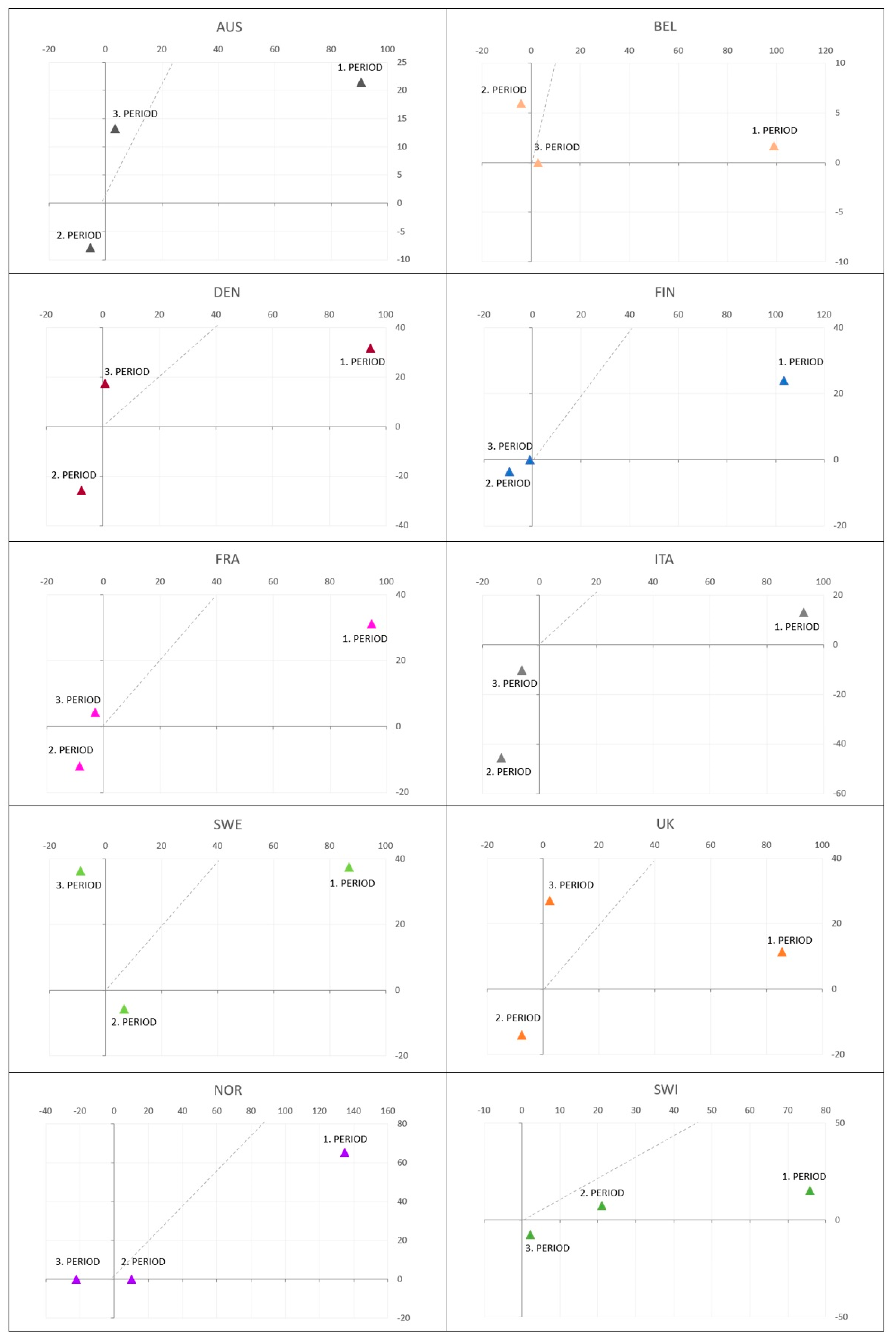
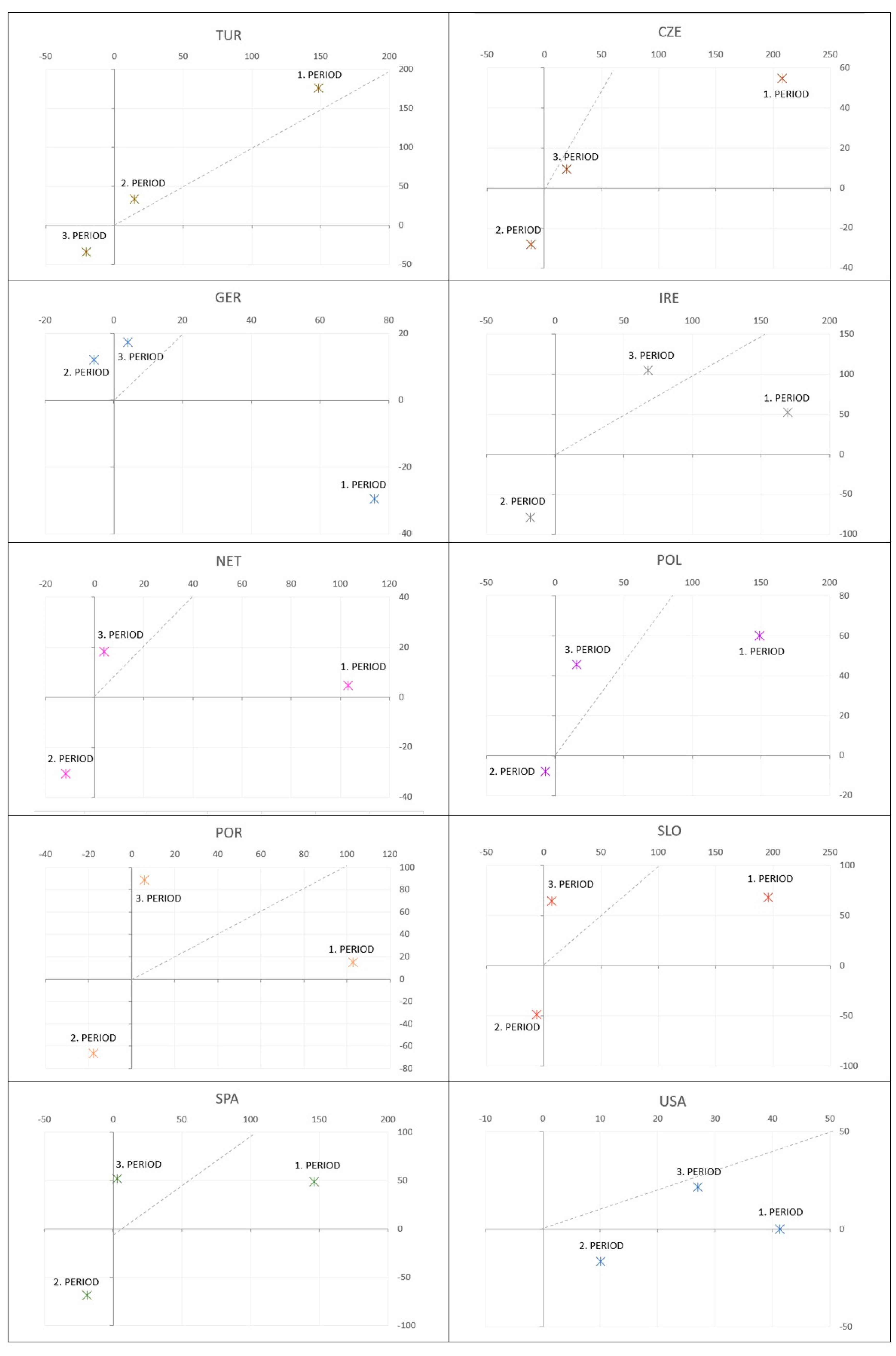
| 1. Period | 2. Period | 3. Period | ||||
|---|---|---|---|---|---|---|
| ΔGDP | ΔCCO2 | ΔGDP | ΔCCO2 | ΔGDP | ΔCCO2 | |
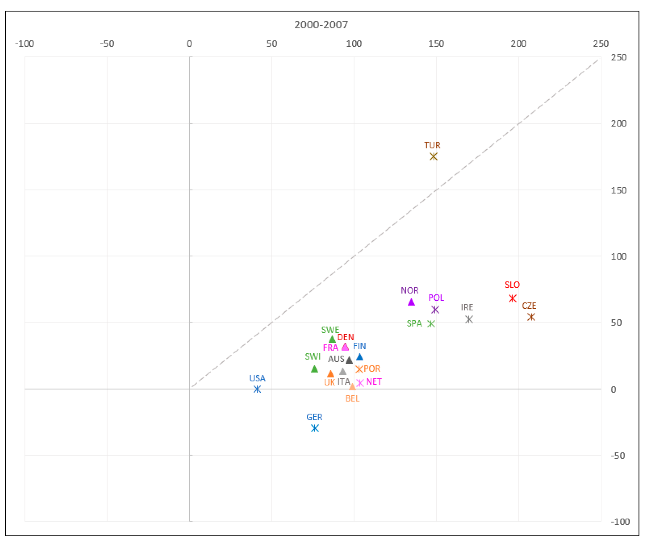
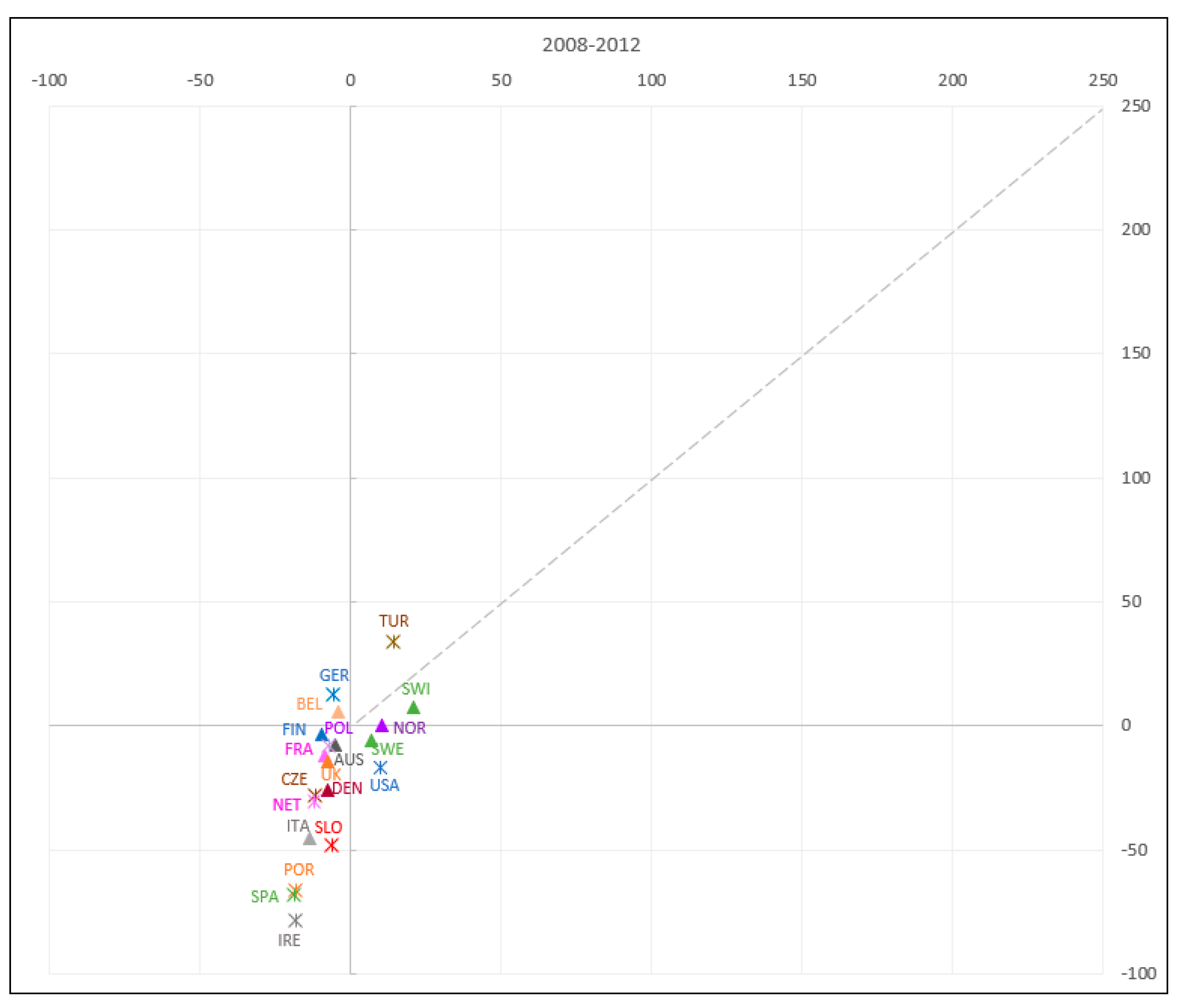
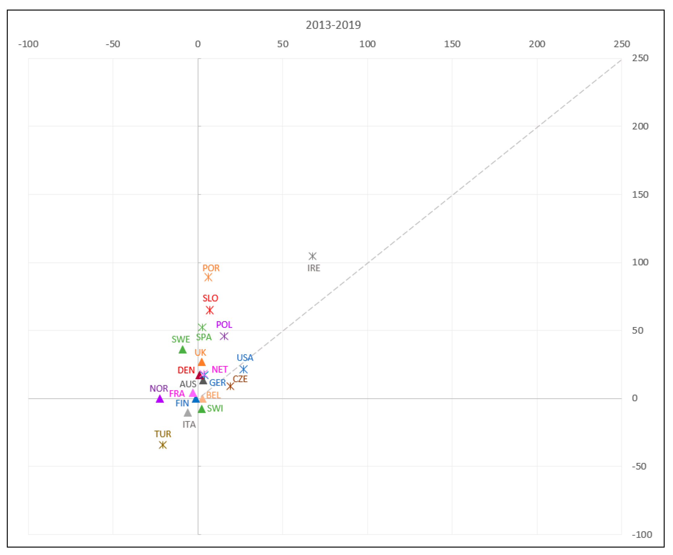
| AUS | 97.27 | 21.51 | −5.24 | −7.83 | 3.35 | 13.33 |
| BEL | 98.88 | 1.69 | −4.09 | 5.93 | 2.70 | 0.00 |
| CZE | 207.60 | 54.55 | −11.81 | −28.13 | 19.30 | 9.23 |
| DEN | 94.58 | 31.82 | −7.42 | −25.93 | 0.85 | 17.39 |
| FIN | 103.44 | 24.00 | −9.60 | −3.57 | −1.05 | 0.00 |
| FRA | 94.82 | 31.20 | −8.42 | −11.99 | −2.95 | 4.40 |
| GER | 75.85 | −29.53 | −5.82 | 12.20 | 4.16 | 17.32 |
| IRE | 169.52 | 52.54 | −18.27 | −79.00 | 67.54 | 104.76 |
| ITA | 93.00 | 13.08 | −13.36 | −45.49 | −6.10 | −10.41 |
| NET | 103.26 | 4.71 | −11.87 | −30.48 | 3.76 | 18.18 |
| POL | 149.11 | 60.00 | −7.19 | −8.02 | 15.57 | 45.56 |
| POR | 102.77 | 15.00 | −17.92 | −66.36 | 5.99 | 88.89 |
| SLO | 196.02 | 68.42 | −6.20 | −48.65 | 6.85 | 64.71 |
| SPA | 146.34 | 48.91 | −18.82 | −68.70 | 2.86 | 52.15 |
| SWE | 86.90 | 37.50 | 6.72 | −5.71 | −9.02 | 36.36 |
| UK | 85.56 | 11.30 | −7.59 | −14.15 | 2.39 | 27.04 |
| NOR | 134.84 | 65.22 | 10.29 | 0.00 | −22.29 | 0.00 |
| SWI | 75.76 | 15.24 | 21.00 | 7.44 | 2.14 | −7.50 |
| TUR | 148.39 | 175.56 | 14.29 | 33.62 | −20.55 | −34.31 |
| USA | 41.20 | 0.00 | 10.05 | −16.66 | 26.94 | 21.73 |
 | 1a | Coupling | GDP > 0 Air Emission > 0 GDP < Air Emission | Positive Growth |
| 1b | Relative Decoupling | GDP > 0 Air Emission > 0 GDP > Air Emission | ||
| 2 | Absolute Decoupling | GDP > 0 Air Emission < 0 | ||
| 3 | Negative Coupling | GDP < 0 Air Emission < 0 | Negative Growth | |
| 4 | Negative Decoupling | GDP < 0 Air Emission > 0 |
Disclaimer/Publisher’s Note: The statements, opinions and data contained in all publications are solely those of the individual author(s) and contributor(s) and not of MDPI and/or the editor(s). MDPI and/or the editor(s) disclaim responsibility for any injury to people or property resulting from any ideas, methods, instructions or products referred to in the content. |
© 2024 by the author. Licensee MDPI, Basel, Switzerland. This article is an open access article distributed under the terms and conditions of the Creative Commons Attribution (CC BY) license (https://creativecommons.org/licenses/by/4.0/).
Share and Cite
Dobrucali, E. Relationship between CO2 Emissions from Concrete Production and Economic Growth in 20 OECD Countries. Buildings 2024, 14, 2709. https://doi.org/10.3390/buildings14092709
Dobrucali E. Relationship between CO2 Emissions from Concrete Production and Economic Growth in 20 OECD Countries. Buildings. 2024; 14(9):2709. https://doi.org/10.3390/buildings14092709
Chicago/Turabian StyleDobrucali, Esra. 2024. "Relationship between CO2 Emissions from Concrete Production and Economic Growth in 20 OECD Countries" Buildings 14, no. 9: 2709. https://doi.org/10.3390/buildings14092709