Nonlinear Seismic Response of Tunnel Structures under Traveling Wave Excitation

Abstract

Tunnels traditionally regarded as resilient to seismic events have recently garnered significant attention from engineers owing to a rise in incidents of seismic damage. In this paper, the reflection characteristics of the elastic plane wave incident on the free surface are analyzed, and the matrix analysis method SWIM (Seismic Wave Input Method) for the calculation of equivalent nodal loads with artificial truncated boundary conditions for seismic wave oblique incidence is established by using coordinate transformation technology, according to the displacement velocity and stress characteristics of a plane wave. The results show that the oblique incidence method is more effective in reflecting the traveling wave effect, and the “rotational effect” induced by oblique incidence must be considered for P wave and SV wave incidence, including the associated stress and deformation. This effect exhibits markedly distinct rotational phenomenon. In particular, the P wave incidence should be focused on the vault and the inverted arch due to the expansion wave. With the increase of the oblique incidence angle, the structural stress and deformation are rotated to a certain extent, and the values are significantly increased. Simultaneously, the shear action of the SV wave may result in “ovaling” of the tunnel structure, thereby facilitating damage to the arch shoulder and the sidewall components. As the oblique incidence angle, the potentially damaging effects of the “rotational effect” to the vault and the inverted arch, but the numerical value does not change significantly. In addition, in comparison to a circular cross-section, the low-frequency amplification of seismic waves in the surrounding rock and the difference of frequency response function in different parts of the lining are more pronounced. In particular, the dominant frequency characteristics are significant at P wave incidence and the seismic wave signal attenuation tends to be obvious with increasing incidence angle. In contrast, SV waves exhibit more uniform characteristics.

1. Introduction

The traditional view posits that underground structures exhibit superior seismic performance compared to above-ground structures, resulting in lesser attention being accorded to the seismic challenges faced by underground engineering [1,2]. However, in recent years, there has been a notable increase in instances of earthquake-induced tunnel damage. For example, the 1995 Great Hanshin earthquake (M = 6.9) in Japan [1], the 1999 Chi-Chi earthquake (M = 7.6) in Taiwan, the 2008 Wenchuan earthquake (M = 8.0) [3], and the 2013 Ya’an earthquake (M = 7.0) all inflicted substantial damage on tunnel structures. Numerous studies have indicated that earthquake damage in tunnels tends to concentrate in areas where ground shaking is exacerbated, typically in proximity to slope sliding (especially at the tunnel portal) and fault zones experiencing shearing [4,5]. In a related research report, Sharma [6] explicitly highlighted the fact that tunnel structures incurred up to 50% damage when subjected to earthquakes with a magnitude exceeding 6.0. It is widely acknowledged that tunnels with a depth of less than 50 m are more susceptible to damage [3]. However, the actual circumstances may be more intricate. The 2008 Longxi Tunnel serves as an illustration; despite having a burial depth of up to 500 m, its lining structure also sustained severe damage, thereby challenging existing theories. Consequently, the investigation of the dynamic interaction between ground vibration and tunnel lining structures is of paramount importance and represents a pertinent yet challenging research topic that engineers have been vigorously pursuing [7,8,9].

Compared to the seismic characteristics of above-ground structures, tunnels and underground structures have two significant characteristics: they are limited by the surrounding soil or rock, and their longitudinal scale is much larger. Specifically, the limitation of the surrounding rock will enhance the seismic capacity of the tunnel structure to a certain extent, while the longitudinal large-scale characteristics require attention to be paid to the seismic wave travelling effect, coherence effect, local site effect, etc., caused by the spatial distribution variability of the rock mass, the change of topography, and the crossing of the geological rapid change zone [10,11]. These factors will cause complex phenomena such as a traveling wave effect, propagation attenuation, frequency variation, and a change in incident angle of the seismic wave, which will affect the seismic performance of a tunnel structure.

Seismic design methods for underground research are categorized into vibration and fluctuation methods [12]. The former focuses on analyzing the dynamic response of underground structures and evaluating the internal forces and deformations of the structures by simplifying the seismic effects into equivalent loads through the equivalent static force method or reaction spectrum method. The fluctuation method is based on fluctuation theory, which considers the propagation characteristics of seismic waves in underground media and analyzes the interactions between seismic waves and structures through numerical simulation. Seismic design loads for underground structures are characterized by the deformation and strain imposed on the structure by the surrounding ground, which is usually due to the interaction between the underground structure and the surrounding ground [8,9]. In contrast, surface structures are designed to withstand inertial forces due to ground acceleration, and when ground shaking is expected to be low or the tunnel is in hard rock (underlain bedrock satisfies the rigidity condition, and infinite lateral extension of the strata is assumed), the free-field ground deformation due to seismic events is neglected, and the tunnel structure adapts satisfactorily to this deformation. Although the vibration method approximation has its limitations, it is based in part on the observation that body waves arriving at the site from the source of disturbance are usually incident almost perpendicularly to the ground, rather than in a straight line from the source to the site [6].

For far-field fluctuations, it is typically assumed that seismic waves are shear or compressional waves incident vertically from below. In contrast, when the seismic source is in proximity to the site, the seismic waves propagate obliquely to the near field at a specific angle, exhibiting spatially varying characteristics. The non-coherent alterations in surface motion induced by the oblique incidence of seismic waves significantly influence the seismic response of the site. Prolonged seismic wave input can result in the structural seismic response being influenced by multiple wave fields [13,14]. Under the assumption of an elastic foundation for the surrounding rock, the fluctuation method input serves as an effective solution to address the traveling wave effect caused by the oblique incidence of seismic waves. The fluctuation method has achieved the separation of free field and scattered field in space, effectively transforming the problem of seismic wave input into an internal source wave problem within the computational domain. This transformation allows for the direct determination of equivalent nodal loads [15,16]. Additionally, there exist indirect methods, such as the one-dimensional equivalent method [17] and the substructure method [18], which provide alternative approaches for solving the problem. In the context of planar problems, the analytical formulas for equivalent nodal loads are relatively straightforward. Recently, scholars have derived the equivalent nodal loads for three-dimensional seismic waves, specifically for P waves [19,20], SV waves [21,22], and SH waves [22,23], under oblique incidence. However, these analytical formulas are quite complex, posing significant challenges for their application in engineering practice. However, research on the spatial non-consistency of ground vibration, the dynamic response of surrounding rock, and the spectral correlation of the seismic dynamic response of tunnel structures remains relatively scarce. In terms of the oblique incidence of 3D seismic waves, the analytical formula for the equivalent nodal load at the truncated boundary of the scattered field is highly complex, limiting its application in engineering practice [24].

In summary, research on the structural response of tunnels under seismic wave action has been fruitful; however, there remain several unresolved scientific issues. For example, how can we evaluate the spatial nonuniformity of the seismic wave input through wave field separation, which partially accounts for traveling wave effects? How can we assess the amplification effect of ground shaking on expansion waves and shear waves with different incidence angles, and its subsequent impact on the spectral correlation of the mechanical response of the lining structure? This paper first analyzes the characteristics of the free surface incident on P and SV waves. Based on the principle of wave field separation, combined with the analytical solution of one-dimensional wave equations and the application of coordinate transformation techniques, this paper develops an equivalent nodal load calculation method for plane wave incidence and extends this method to the three-dimensional seismic wave model. Furthermore, the static mechanics of tunnel excavation and seismic dynamics analysis are effectively integrated by introducing the birth–death element technique and boundary condition transformation. The reliability of the method is verified through numerical examples. Meanwhile, the time-dependent response of rock displacement under traveling wave effects is analyzed, and preliminary insights are gained into the spatial coherence of ground vibration at the site under the condition of oblique incidence of seismic waves, as well as the nonlinear dynamic response behavior of noncircular tunnel structures.

2. Seismic Wave Reflection Theory

2.1. Plane Wave Reflection Theory

According to the elastic wave theory [25,26], in the context of a planar scenario, seismic waves are differentiated into longitudinal waves (P waves or compression–expansion waves) and transverse waves (SH waves and SV waves, which signify horizontal and vertical shear waves, respectively). Utilizing the P wave as an exemplary case, the wave functions corresponding to the incident P wave, reflected P wave, and reflected SV wave can be articulated as follows,

$${\varphi }_p^i=A_p^i\exp \left[\mathrm{i}{\omega }_p\left(-{\displaystyle \frac{x}{c_p}}\sin \alpha +{\displaystyle \frac{y}{c_p}}\cos \alpha +t\right)\right],$$

(1)

$${\varphi }_p^r=A_p^r\exp \left[\mathrm{i}{\omega }_p\left(-{\displaystyle \frac{x}{c_p}}\sin {\alpha }^{\prime }-{\displaystyle \frac{y}{c_p}}\cos {\alpha }^{\prime }+t\right)\right],$$

(2)

$${\varphi }_s^r=A_s^r\exp \left[\mathrm{i}{\omega }_s\left(-{\displaystyle \frac{x}{c_s}}\sin \beta -{\displaystyle \frac{y}{c_s}}\cos \beta +t\right)\right].$$

(3)

The wave function $\varphi$ describes the propagation characteristics of the wave, including the amplitude $A$, frequency $\omega$, wave speed $c$, and wave shape. Among these parameters, the superscript $i,r$ denotes the incident wave and reflected wave; the subscript $p,s$ indicates the P wave and SV wave; $t$ represents the time; and $\alpha ,{\alpha }^{\prime },\beta$ is the angle of the incident P wave, the reflected P wave, and the reflected SV wave, respectively (as depicted in Figure 1 for plane waves). In the free interface with no medium, the displacement continuity condition is no longer applicable due to the absence of adjacent medium transferring the stress, and the stress is equal to zero here. Substituting the three wave functions in Equations (1)−(3) into the stress boundary, it can be deduced that the reflected wave and the incident wave must have the same frequency. At the same time, the projection of the wave vectors of the reflected and incident waves on the interface, that is, the apparent wave number, must also be the same [25], expressed in the form of Snell’s law:

$${\displaystyle \frac{\sin \alpha }{c_p}}={\displaystyle \frac{\sin {\alpha }^{\prime }}{c_p}}={\displaystyle \frac{\sin \beta }{c_s}}.$$

(4)

The angles of reflection of an incident P wave and a reflected P wave are the same, $\alpha ={\alpha }^{\prime }$; the angle of reflection of a reflected SV wave is smaller than the angle of reflection of a reflected P wave, $\beta <\alpha$. During wave propagation, the frequency of the wave and the projection of the wave front onto the interface (apparent wave number) remain invariant, although the direction may change. Meanwhile, the reflection coefficients (the ratio of the displacement amplitude of the reflected wave to that of the incident wave) are $A_{pp}={\displaystyle \frac{A_p^r}{A_p^i}}\cdot {\displaystyle \frac{c_p}{c_p}}={\displaystyle \frac{c_s^2\sin 2\alpha \sin 2\beta -c_p^2{\cos }^{2}2\beta }{c_s^2\sin 2\alpha \sin 2\beta +c_p^2{\cos }^{2}2\beta }}$, $A_{sp}={\displaystyle \frac{A_s^r}{A_p^i}}\cdot {\displaystyle \frac{c_p}{c_s}}={\displaystyle \frac{2c_s{c}_p\sin 2\alpha \cos 2\beta }{c_s^2\sin 2\alpha \sin 2\beta +c_p^2{\cos }^{2}2\beta }}$. From an energy point of view, the energy flow reflection coefficients are $R_{pp}=(A_{pp}{)}^2$, $R_{sp}=(A_{sp}{)}^2{\displaystyle \frac{c_s\cos \beta }{c_p\cos \alpha }}$. The same method is used for the incident SV wave; for further details, refer to Appendix A.

2.2. Seismic Wave Reflection Discussion

Figure 2 illustrates the change pattern of the reflection coefficient for a plane wave incident on a free surface. From Figure 2, it can be seen that, with the gradual increase of the P wave incident angle, the reflection coefficient of the reflected P wave is predominantly negative, indicating that a significant shift in the polarization direction occurs at the free surface. At the same time, the phenomenon of half-wave loss occurs in this phase. The trend of the reflection coefficient shows a pattern that is decreasing and then increasing. In particular, when the angle of incidence is 0 degrees, the reflection coefficient reaches 1, indicating that the reflected wave consists only of P waves and the amplitude of the free surface displacement is twice the amplitude of the incident wave. When µ is small enough (about 0.25, which is related to the incident angle and the wave velocity ratio), it is possible for the reflected P wave to change its direction, and there always exists an angle that makes the reflection coefficient positive [26]. Meanwhile, the behavior of the reflected SV wave differs, as shown in Figure 2. Under the regular Poisson’s ratio condition, the reflection coefficient is consistently negative. When the angle of incidence is 90 degrees, the wave advances in a direction parallel to the boundary, a state known as grazing incidence. In this state, the total displacement everywhere is constantly equal to 0, which is physically unattainable and is merely a virtual state [27]. It is physically unrealizable and exists only as a virtual state. Under certain specific conditions (indicated by the point where the black dashed lines intersect in Figure 2), the reflection coefficient is zero, and the reflected field consists only of SV waves, despite the incident P wave. This indicates that the phenomenon of waveform conversion has occurred.

According to Snell’s theorem, the angle of incidence of an SV wave is always less than the angle of egress of a reflection-converted P wave. Therefore, there exists a critical angle of incidence for SV waves, $\alpha =\arcsin (c_s/c_p)$. Figure 3 shows that the reflection coefficient is 0 when the angle of incidence exceeds this angle, a situation beyond the scope of this paper. Similar to P wave incidence, the reflection coefficient of the reflected SV wave is generally negative and will be equal to 0 under some specific conditions, when the reflected wave from SV incidence will be completely converted to a P wave. When the angle of incidence is 0 degrees (vertical incidence), the reflection coefficient is 1, which means that the only reflected wave is the SV wave, and the amplitude of the free surface displacement is twice the amplitude of the incident wave. It should be noted with caution that the reflected P wave may have a very high reflection coefficient, even much higher than 1. When the angle of incidence is equal to 45 degrees, the reflection coefficient is 0, and there is only a reflected SV wave with a constant phase.

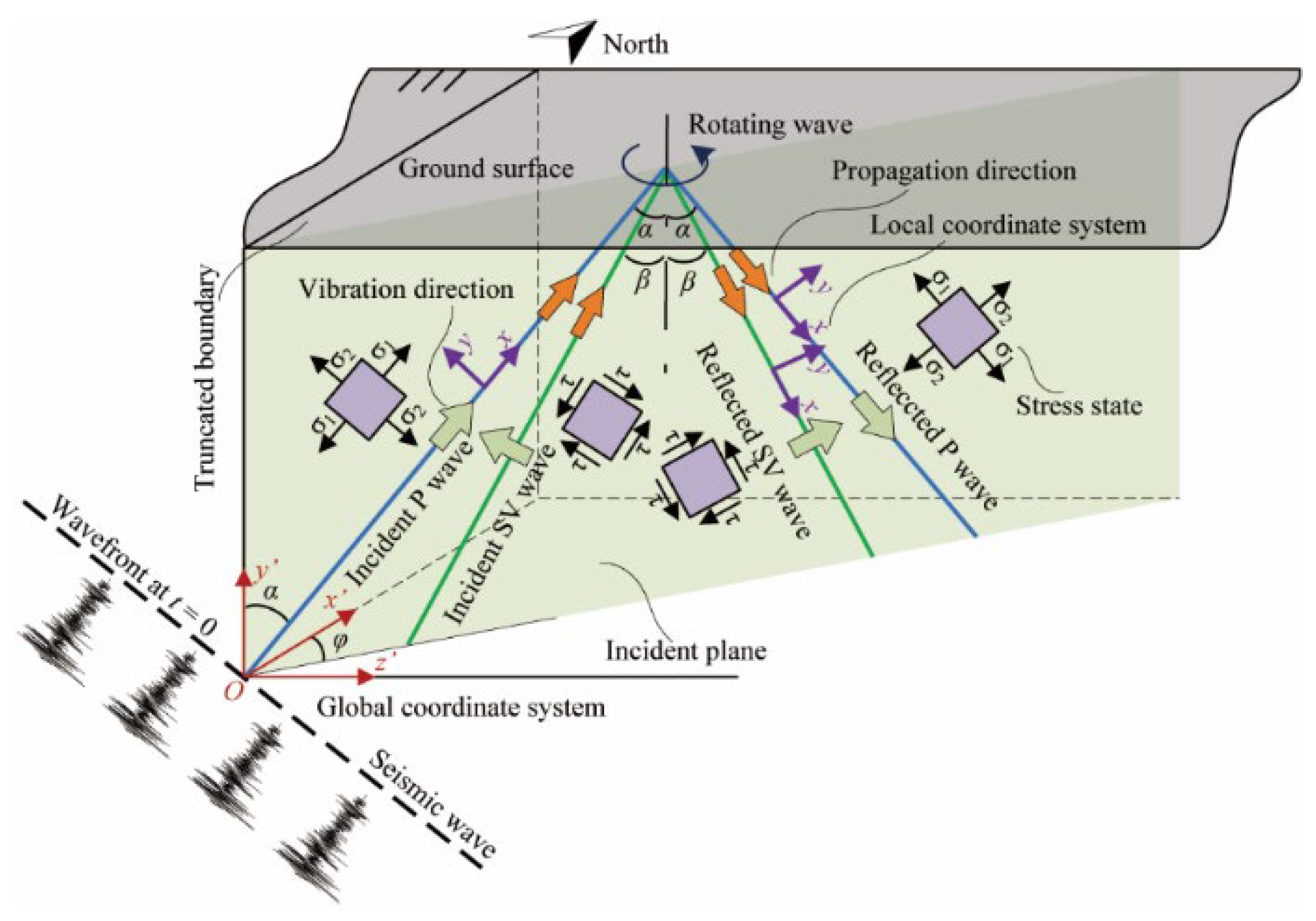
3. Theory of Seismic Wave Incidence

3.1. Matrix Methods for Coordinate Transformations

During the propagation of plane waves, the wave field displacement is written as $\mathit{u}={\mathit{u}}_p+{\mathit{u}}_s=\nabla \phi +\nabla \times \mathit{\Psi }$; the former scalar $\nabla \phi$ is the fluctuation equation of compression waves, and the latter vector $\nabla \times \mathit{\Psi }$ is the fluctuation equation of shear waves. The plasmonic vibration of the P wave and propagation direction are consistent, the plasmonic vibration of the SV wave and the propagation direction are perpendicular, and the P wave and the SV wave are coupled in the plane. In order to simplify the analysis, a suitable local coordinate system was established to reduce the seismic wave into a one-dimensional fluctuation problem, which was expanded into a plane or a three-dimensional space by a coordinate transformation matrix, thereby avoiding complex calculation formulas and aiding in a deeper understanding of the propagation mechanism and properties of the waves.

(1)

Acceleration, velocity, displacement:

According to the plane wave property, the P wave generates line displacement only in its vibration direction. In order to simplify the analysis, the local coordinate system x-axis was set in the vibration direction of the mass, both P wave and SV wave, $u_x^i(t)\ne 0$, $u_y^i(t)=0$. The plane wave is reduced to a one-dimensional fluctuation problem, which greatly simplifies the processing and calculation of physical quantities. Taking the P wave as an example (see Appendix B for the SV wave), in the simplified one-dimensional model, the displacement of any point contains three parts, the incident P wave, the reflected P wave, and the reflected SV wave (denoted by i = 1, 2, 3). For the coordinate transformation matrix, shown in Figure 1, the purple local coordinate system (incident direction x, vertical direction y) is transformed to the overall coordinate system cyan plane (origin O, horizontal x, vertical y) in the case of an incident P wave, ${\Phi }_1=\left[\begin{array}{cc}\sin \alpha & -\cos \alpha \\ \cos \alpha & \sin \alpha \end{array}\right]$. Using the same method, the reflected P wave and reflected SV wave transformation matrices can be derived, ${\Phi }_2,{\Phi }_3$. Using the Einstein summation markers, the displacement of any point in the model is expressed as:

$$\overline{\mathit{u}}={\Phi }_i{\mathit{u}}_i,$$

(5)

$$\begin{array}{ll}\left[\begin{array}{c}{u}_x(t)\\ u_y(t)\end{array}\right]& =\left[\begin{array}{cc}\sin \alpha & -\cos \alpha \\ \cos \alpha & \sin \alpha \end{array}\right]\left[\begin{array}{c}{u}_x^{ip}(t-t_1)\\ u_y^{ip}(t-t_1)\end{array}\right]\\ & +\left[\begin{array}{cc}\sin \alpha & \cos \alpha \\ -\cos \alpha & \sin \alpha \end{array}\right]\left[\begin{array}{c}{u}_x^{rp}(t-t_2)\\ u_y^{rp}(t-t_2)\end{array}\right]+\left[\begin{array}{cc}\sin \beta & \cos \beta \\ -\cos \beta & \sin \beta \end{array}\right]\left[\begin{array}{c}{u}_x^{rs}(t-t_3)\\ u_y^{rs}(t-t_3)\end{array}\right],\end{array}$$

(6)

where $\overline{\mathit{u}},{\mathit{u}}_i$ are the displacement vectors of the overall and local coordinate systems, respectively; due to the difference in the arrival time of the incident wave and the reflected wave at the same point, the time delays caused by the traveling wave effect are as follows: $t_1={\displaystyle \frac{x\sin \alpha +y\cos \alpha }{c_p}}$, $t_2=t_1+{\displaystyle \frac{\left(2h-y\right)\cos \alpha }{c_p}}$, $t_3=t_1+\left(h-y\right)\left({\displaystyle \frac{\cos (\alpha +\beta )}{c_p\cos \beta }}+{\displaystyle \frac{1}{c_s\cos \beta }}\right)$. h stands for the overall model height, and y is the vertical coordinate of the point. The derivation of the delay time will not be repeated, and the detailed process can also be found in Reference [22].

(2)

Stress and strain

When the velocity of the plasma is much smaller than the propagation velocity of the wave in the medium, the fluctuation phenomenon can be analyzed using the theory of linear elasticity. The plane wave displacement is derived for time and space, and a simplified one-dimensional fluctuation equation can be obtained, ${\displaystyle \frac{\mathsf{\partial }u}{\mathsf{\partial }x}}=-{\displaystyle \frac{1}{c}}{\displaystyle \frac{\mathsf{\partial }u}{\mathsf{\partial }t}}$. Within the local coordinate system, when the P wave propagates, the vibration direction and propagation direction of the plasma point are in the x-axis. Therefore, the P wave can only produce displacement in the x-direction $u_x(t)\ne 0$, while the displacement component in the y-direction is 0. According to the geometric equations in elastic dynamics ${\epsilon }_{ij}={\displaystyle \frac{1}{2}}\left({\mathit{u}}_{i,j}+{\mathit{u}}_{j,i}\right)$, the strain corresponding to the P wave incidence is deduced, and only the x-direction line strain is not equal to 0, ${\epsilon }_x={\displaystyle \frac{\mathsf{\partial }{u}_x}{\mathsf{\partial }x}}=-{\displaystyle \frac{1}{c_p}}{\displaystyle \frac{\mathsf{\partial }{u}_x}{\mathsf{\partial }t}}$, while the y-direction line strain and shear strain are both 0: ${\epsilon }_y={\gamma }_{xy}=0$. The strains can be written in the form of a matrix,

$${\epsilon }_{ij}=\left[\begin{array}{cc}-{\displaystyle \frac{1}{c_p}}{\displaystyle \frac{\mathsf{\partial }{u}_x}{\mathsf{\partial }t}}& 0\\ 0& 0\end{array}\right]$$

(7)

According to Hooke’s law for ideal elastomers, the physical equation of the surrounding rock material can be written as ${\mathit{\sigma }}_{ij}=2G{\epsilon }_{ij}+\lambda {\epsilon }_{kk}{\mathit{\delta }}_{ij}$, and the joint physical and geometric equations as ${\mathit{\sigma }}_{ij}=G\left({\mathit{u}}_{i,j}+{\mathit{u}}_{j,i}\right)+\lambda {\epsilon }_{kk}{\mathit{\delta }}_{ij}$, where ${\mathit{\delta }}_{ij}$ is the Kronecker function, $G={\displaystyle \frac{E}{2\left(1+\mu \right)}}$, $\lambda ={\displaystyle \frac{E\mu }{\left(1+\mu \right)\left(1-2\mu \right)}}$, $G$ is the shear modulus, and $\lambda ,\mu$ is the Lame’s constant. Substituting strain Equation (7) into the physical equation, it is found that only positive stresses exist, while the shear stresses are all zero, ${\mathit{\sigma }}_{ij}=0, i\ne j$. The stresses in the incident P wave can be written in matrix form as

$${\mathit{\sigma }}_p^i=\left[\begin{array}{cc}{\sigma }_x& 0\\ 0& {\sigma }_y\end{array}\right]=\left[\begin{array}{cc}(\lambda +2G){\epsilon }_x& 0\\ 0& \lambda {\epsilon }_x\end{array}\right].$$

(8)

Using the Einstein summation markers, the stress at any point in the overall coordinate system is expressed as:

$$\overline{\mathit{\sigma }}={\Phi }_i^T{\mathit{\sigma }}_i{\Phi }_i,$$

(9)

where $\overline{\mathit{\sigma }},{\mathit{\sigma }}_i$ are the stresses in the overall and local coordinate systems, respectively. It is worth noting that the displacements are vectors, and conform to the linear transformation rules for vectors, while the stresses need to follow the second-order tensor coordinate transformation rules [28].

(3)

Equivalent Nodal Load

According to the wave field separation principle, the fluctuating field of the soil structure is decomposed into free and scattered fields, and the equivalent nodal force at the artificial truncated boundary is calculated as

$$\mathit{F}(t)={\mathit{f}}_b+{\mathit{R}}_b=\left(K{\mathit{u}}_b+C{\dot{\mathit{u}}}_b+{\mathit{\sigma }}_b\mathit{n}\right)A_b+{\mathit{R}}_b,$$

(10)

where ${\mathit{f}}_b$ is the equivalent nodal load of the seismic fluctuation input, $K$ is the stiffness matrix, $C$ is the damping matrix, ${\mathit{u}}_b$${\dot{\mathit{u}}}_b$ represents the displacements and velocities of the overall coordinate system (for simplicity of representation, we will ignore the underlined markings of the overall coordinates), ${\mathit{\sigma }}_b$ is the stresses, $A_b$ is the impact area, and $\mathit{n}$ is the normal vector. ${\mathit{f}}_b$ contains two parts, where the first two represent the nodal force needed by the scattered field to resist the artificial boundary ${\mathit{f}}_{b1}$, and the third is the nodal force of the scattered field to resist the near-field medium ${\mathit{f}}_{b2}$. ${\mathit{R}}^f$ is the constraint reaction force for the static-to-power artificial boundary. In order to effectively simulate the seismic wave propagation at infinity and prevent the wave field from generating unreasonable reflection and bypassing phenomena at the boundary, artificial viscous boundary conditions are adopted at the truncated boundary, and the spring stiffnesses are respectively set as [14]. The spring stiffness is set as follows:

$$k_n={\displaystyle \frac{1}{1+a}}{\displaystyle \frac{\lambda +2G}{r}}, c_n=b\rho c_p,$$

(11)

$$k_t={\displaystyle \frac{1}{1+a}}{\displaystyle \frac{G}{r}}, c_t=b\rho c_s,$$

(12)

where $k_n,k_t,c_n,c_t$ is the normal and tangential spring stiffness coefficients, $r$ is the distance from the wave source to the artificial boundary node, and $c_p,c_s$ is the wave speed. $G$ is the shear modulus, $\lambda$ is the Lame constant, and $\rho$ density. $a,b$ is the damping coefficient [20], with values ranging from [0.5 1.0], [1.0 2.0].

In setting up the artificial boundary, the viscous damper is independent of the distance from the scattering wave source to the artificial boundary, but the stiffness of the spring is related to it. The scattering source in real problems is not a point source, but a spatially distributed line or surface source. Therefore, it can only be chosen in an average sense, considering the shortest distance from the geometric center of the structure to the artificial boundary [21]. The artificial viscous boundary is set up with two directional springs to model stiffness and damping, denoted as n in the outer normal direction and t in the tangential direction. Substituting the stiffness matrix and the viscous matrix, $K=\left[\begin{array}{cc}{k}_n& k_t\\ k_t& k_n\end{array}\right]$$C=\left[\begin{array}{cc}{c}_n& c_t\\ c_t& c_n\end{array}\right]$, into Equation (10) yields that

$${\mathit{f}}_b=K\mathit{n}{A}_b{\mathit{u}}_b+C\mathit{n}{A}_b{\dot{\mathit{u}}}_b+{\mathit{\sigma }}_b\mathit{n}{A}_b,$$

(13)

$$\left\{\begin{array}{c}{f}_x\\ f_y\end{array}\right\}=\left[\begin{array}{cc}{k}_n& k_t\\ k_t& k_n\end{array}\right]\left[\begin{array}{c}-A_b\\ 0\end{array}\right]\left\{\begin{array}{c}{u}_x\\ u_y\end{array}\right\}+\left[\begin{array}{cc}{c}_n& c_t\\ c_t& c_n\end{array}\right]\left[\begin{array}{c}-A_b\\ 0\end{array}\right]\left\{\begin{array}{c}{\dot{u}}_x\\ {\dot{u}}_y\end{array}\right\}+\left[\begin{array}{cc}{\sigma }_x& {\tau }_{xy}\\ {\tau }_{yx}& {\sigma }_y\end{array}\right]\left[\begin{array}{c}-A_b\\ 0\end{array}\right]$$

(14)

3.2. Extension to 3D Modeling

When dealing with seismic wave propagation and geological characterization, the reasonable conversion of coordinate system is crucial. In this paper, two approaches to coordinate conversion are proposed: to establish the coordinate system in the plane first and then extend it to 3D, or to carry out 3D coordinate transformation directly. Based on the theory of plane fluctuation described in Section 3.1, this paper establishes the overall coordinate system of $x^{\prime }{y}^{\prime }{z}^{\prime }$ shown in Figure 1 according to the right-hand rule in order to accurately describe the geological features such as joints and faults. The local coordinate system is in the cyan plane, and the projection vector of the $x$ axis in the overall coordinate system is ${\overline{\mathit{e}}}_{\mathit{x}}=\{\cos \varphi ,0,-\sin \varphi \}$, where $\varphi$ is the angle between the incident surface in the horizontal projection and the north direction, and the value range is $\left[0,\pi \right]$ to avoid the seismic wave incident direction deviating from the numerical model.

According to the geometric space vector relationship, ${\overline{\mathit{e}}}_z={\displaystyle \frac{{\overline{\mathit{e}}}_x\times {\mathit{e}}_y}{\left|{\overline{\mathit{e}}}_x\times {\mathit{e}}_y\right|}}=\{\sin \varphi ,0,\cos \varphi \}$, we obtain the $y$ axis projection ${\overline{\mathit{e}}}_y={\overline{\mathit{e}}}_z\times {\overline{\mathit{e}}}_x=\{0,1,0\}$. Then the conversion matrix of the 2D plane to the 3D model is as follows:

$$\overline{\mathit{u}}={\left[\begin{array}{ccc}{\overline{u}}_x& {\overline{u}}_y& {\overline{u}}_z\end{array}\right]}^T={\Phi }^T\mathit{u}={\left[\begin{array}{c}{\overline{\mathit{e}}}_x\\ {\overline{\mathit{e}}}_y\\ {\overline{\mathit{e}}}_z\end{array}\right]}^T\left[\begin{array}{c}{u}_x\\ u_y\\ u_z\end{array}\right]={\left[\begin{array}{ccc}\cos \varphi & 0& -\sin \varphi \\ 0& 1& 0\\ \sin \varphi & 0& \cos \varphi \end{array}\right]}^T\left[\begin{array}{c}{u}_x\\ u_y\\ u_z\end{array}\right],$$

(15)

which is available at $u_{y^{\prime }}=0$. The stresses then need to follow the second-order tensor coordinate transformation rules,

$$\overline{\mathit{\sigma }}={\Phi }^T\mathit{\sigma }\Phi ={\left[\begin{array}{ccc}\cos \varphi & 0& -\sin \varphi \\ 0& 1& 0\\ \sin \varphi & 0& \cos \varphi \end{array}\right]}^T\left[\begin{array}{ccc}{\sigma }_x& {\tau }_{xy}& 0\\ {\tau }_{yx}& {\sigma }_y& 0\\ 0& 0& 0\end{array}\right]\left[\begin{array}{ccc}\cos \varphi & 0& -\sin \varphi \\ 0& 1& 0\\ \sin \varphi & 0& \cos \varphi \end{array}\right].$$

(16)

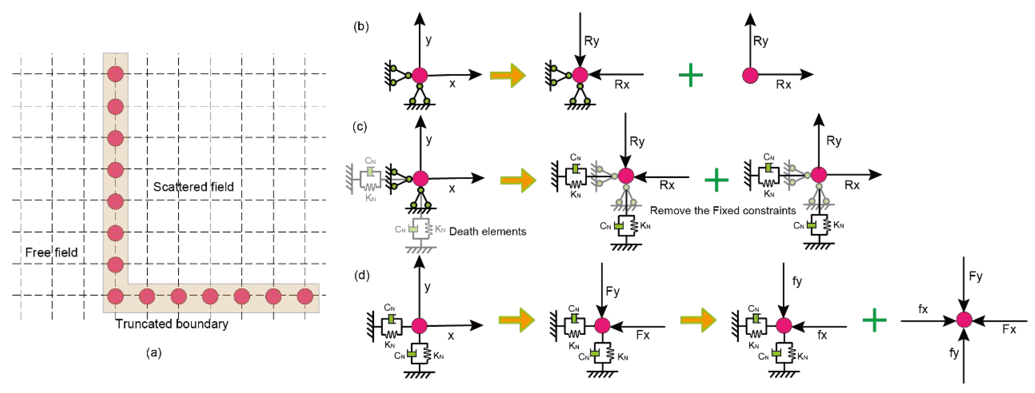
3.3. Transformation of Static and Dynamic Boundary Conditions

In the traditional method, static and dynamic problems are typically calculated separately, and then the results of these two calculations are superimposed. This approach is feasible for static–dynamic combined problems within the scope of linear elasticity and small deformation. However, for nonlinear or large deformation static–dynamic problems, the simple superposition principle becomes inapplicable [29]. Currently, there are three primary methods for static–dynamic boundary transformation, which include: (a) unified boundary conditions for static–dynamic coupled analysis, utilizing the robustness of the viscoelastic boundary to unify the static–dynamic boundary conditions by adjusting the elastic coefficient [30], although there is a certain deviation in the hydrostatic analysis [31]; (b) calculation of static response by kinetic solution, where the static load is considered as a step load applied at zero load [31], and due to the damping effect of the model, the dynamic response induced by the step load decays rapidly and reaches equilibrium [32]; and (c) upon completion of static analysis, the static boundary is converted to a dynamic boundary, followed by dynamic analysis. In this study, the transient dynamic approximation simulation of static conditions (with time integration simulation of static conditions turned off, and time setting at 1 × 10⁻⁵) and life and death unit conversion constraint methods (ekill and ealive) were employed. Figure 3 illustrates the analysis steps as follows: (a) the truncated boundary applied fixed constraints and spring-damped units; (b) the spring-damped units were deactivated, static loads were applied, and the tunnel excavation process was simulated; (c) the fixed constraints at the nodes of the truncated boundary were removed, the spring-damped units were activated, and the equivalent constraint reaction force was applied; and (d) seismic dynamic loads were applied, and dynamics analysis was performed.

In this study, the ANSYS 19.2 numerical analysis software was initially employed to construct the physical model, perform meshing, and export crucial boundary node information, including node identification numbers, precise node coordinates, and designated impact zones. Following this, the MATLAB R2020a programming environment was utilized to develop the computational code SWIM (Seismic Wave Input Method), specifically tailored to generate equivalent boundary loads at the periphery of the seismic wave field. Furthermore, the ANSYS setup solver was invoked to apply artificial viscous boundary conditions, augmented with these equivalent nodal loads, for comprehensive solution derivation. Ultimately, the computational outputs were exported for rigorous data processing and in-depth analysis.

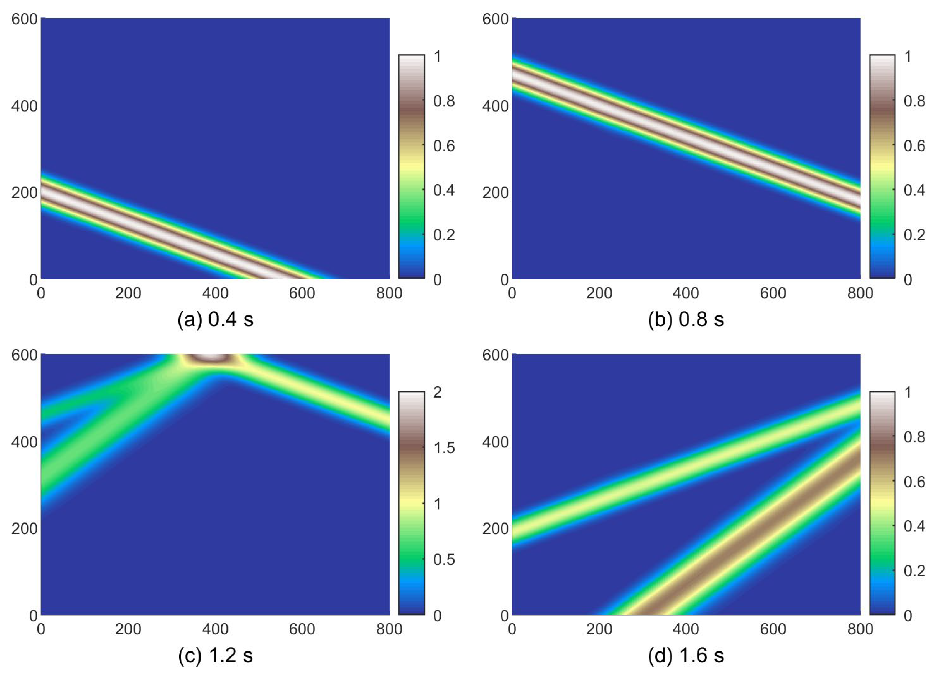
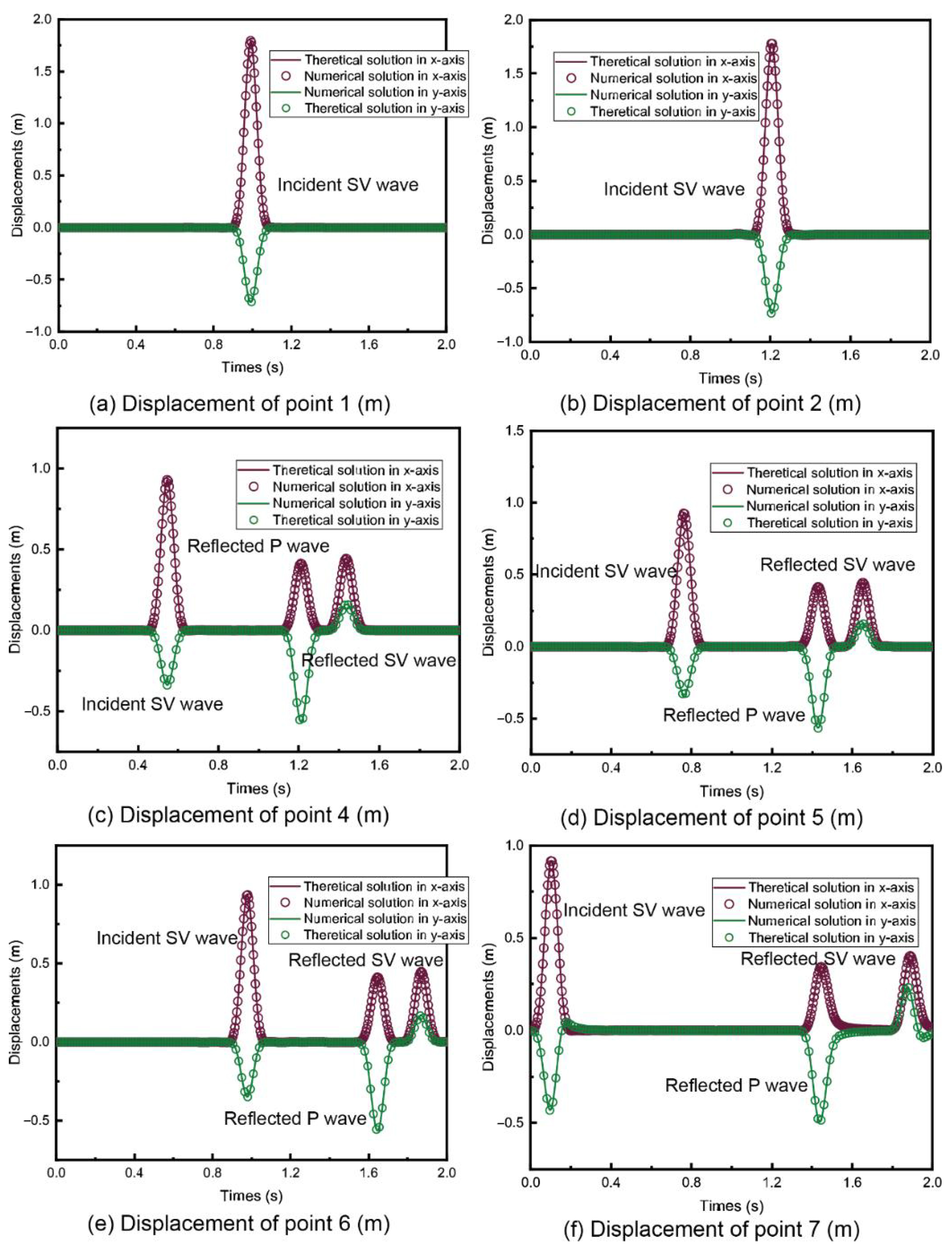
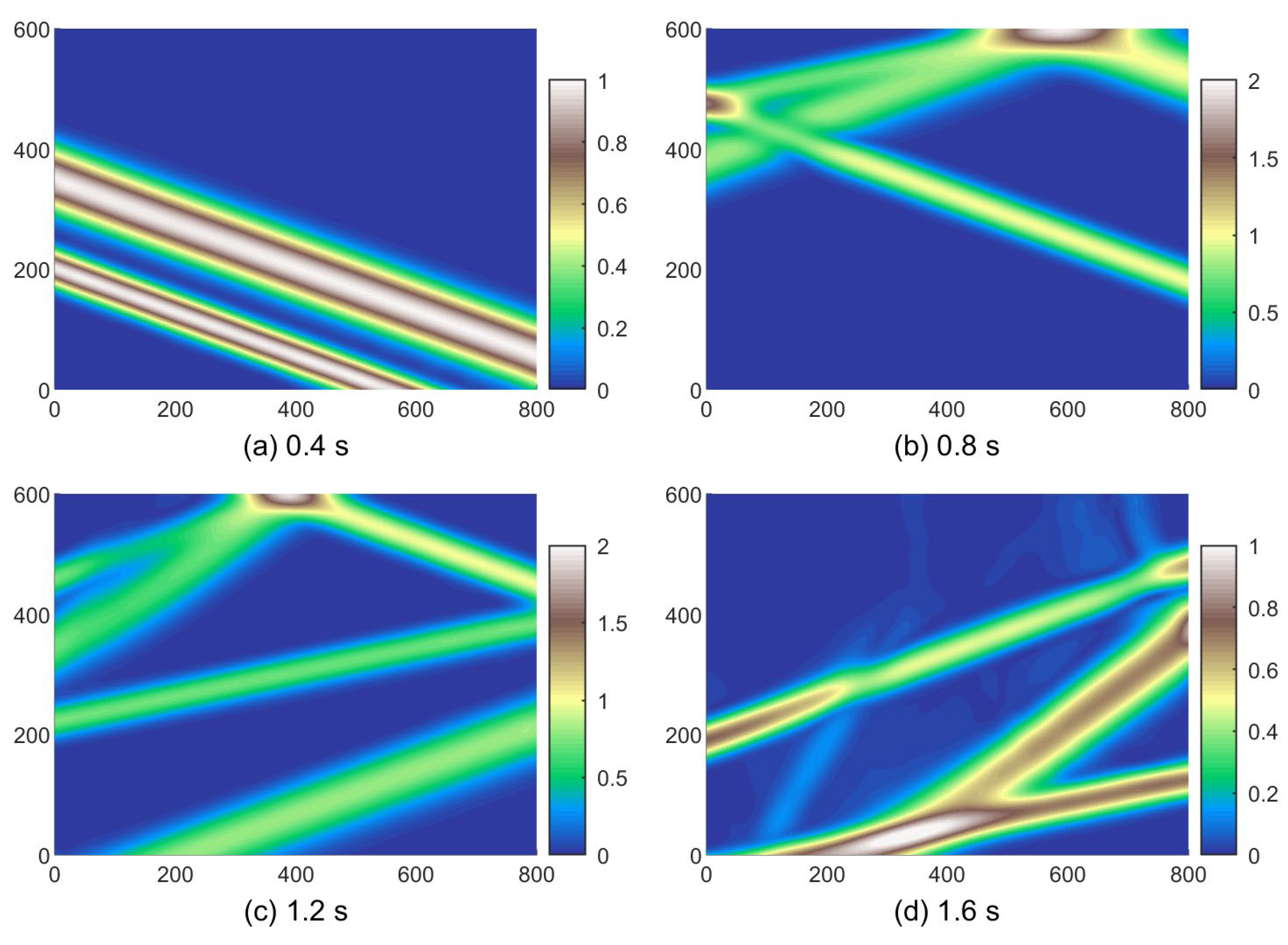
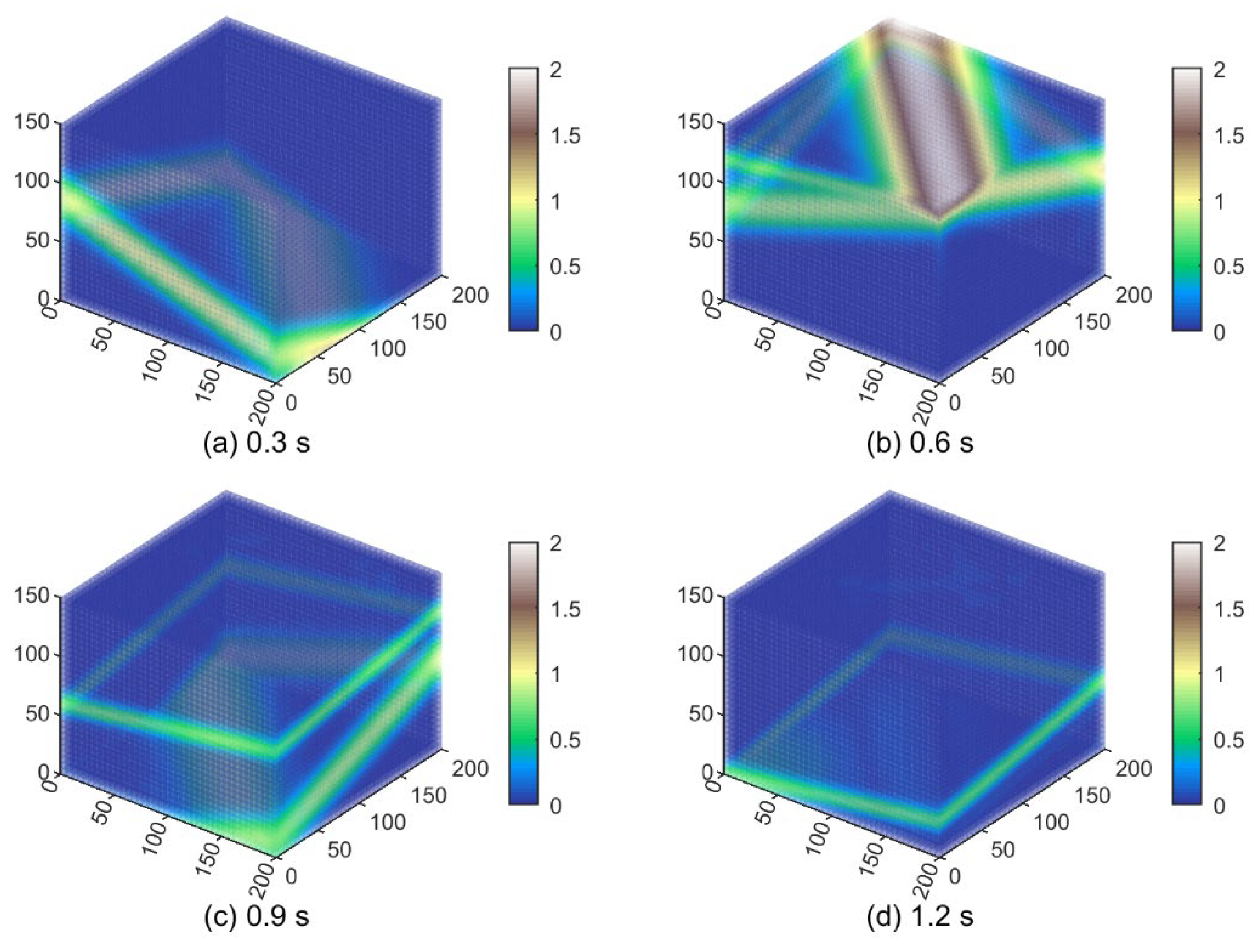
4. Example Validation

In order to verify the reliability of the above theory and compiled code, several simple cases were selected for the algorithm. The main physical model parameters were model size, $800\times 600 \mathrm{m}$; elastic modulus, $E=2\times {10}^9 \mathrm{Pa}$; Poisson’s ratio, $\mu =0.25$; density, $\mathrm{\rho }=2000 \mathrm{kg}\cdot {\mathrm{m}}^{-3}$; artificial viscoelastic boundary parameters, $a=0.8; b=1.1$; mesh size, $5 \mathrm{m}$; and time step, $0.002 \mathrm{s}$. The seismic wave displacement pulse expression is given by:

$$u(t)=16\delta \left[G(t)-4G(t-0.25)+6G(t-0.5)-4G(t-0.75)+G(t-1)\right],$$

(17)

where $\delta$ is the peak value of the unit pulse, taken as 1.0 m; $t={\displaystyle \frac{t_0}{T}}$, $T$ is the action time of the unit pulse; $G(x)=x^{3}H(x)$; and $H(x)$ is the Heaviside step function. Liu et al. [18] considered that to obtain reliable numerical results at a wavelength of $\lambda$, the size of the finite element network should be taken as $\left(1/12\sim 1/6\right)\lambda$.

Figure 4 depicts the displacement propagation characteristics when subjected to oblique incidence of the P wave. By setting the incident angle to 25° and the amplitude to 1.0 m, it was evident that the maximum amplitude escalated to 2.0 m upon the wave’s interaction with the free surface, due to the superposition effect of the reflected wave. The disparity in wave speeds, represented by a ratio of approximately cp/cs = 2.0, is reflected in the widths of the waveforms presented in the figure. In this scenario, the amplitude coefficients for the reflected P wave and reflected SV wave were determined to be A1 = −0.73 and A2 = 0.87, respectively. It is worth noting that the amplitude ratio of the reflected P wave, propagating in the opposite direction to the incident P wave, reached 0.73. Conversely, the amplitude variation coefficient of the reflected SV wave, moving in the same direction as the incident P wave, was 0.87.

On the other hand, Figure 5 illustrates the displacement propagation pattern of SV waves when they encounter oblique incidence conditions. Specifically, when an SV wave propagated with an incidence angle of 20° and an amplitude of 1.0 m, a notable phenomenon occurred: upon reaching the free surface, the superposition of reflected waves resulted in an amplitude peak of 2.0 m. Under these conditions, precise measurements revealed that the amplitude coefficients of the reflected SV wave and the reflected P wave were A1 = −0.59 and A2 = 0.64, respectively. It is worth noting that the propagation direction of the reflected SV wave was opposite to that of the incident SV wave, with an amplitude ratio of 0.59. Conversely, the reflected P wave propagated in the same direction as the incident SV wave, exhibiting an amplitude variation coefficient of 0.64.

To facilitate a comprehensive analysis of the calculation results, we adopted a systematic approach for selecting feature points. These points were chosen sequentially from the top (i.e., the surface), middle, and bottom of the model. Specifically, we initially selected feature points at the top in the left, middle, and right positions. This process was then repeated for corresponding positions in the middle and bottom of the model, resulting in a total of nine feature points. This strategy enabled a more thorough examination of the model’s responses at various depths and locations.

Figure 6 illustrates the displacement of soil feature points over time due to the oblique incidence of SV waves. It is evident that the displacement in the x-direction was positive, while the displacement in the y-direction was the opposite. Furthermore, the displacement in the x-direction was significantly larger than that in the y-direction. These findings are highly consistent with the analytical solution, demonstrating excellent matching accuracy. Notably, the site fluctuations at different feature points varied distinctly due to the traveling wave effect. Additionally, there was a pronounced wave-absorbing effect at the tail, further validating the reliability of the imposed artificial viscous boundary.

Since P and SV waves have a wave speed ratio ${\displaystyle \frac{c_p}{c_s}}={\displaystyle \frac{\sin \alpha }{\sin \beta }}=\sqrt{{\displaystyle \frac{2\left(1-\mu \right)}{1-2\mu }}}$ and $c_p>c_s$, it follows that $\alpha >\beta$. When P and SV waves are incident simultaneously, their incident angles are not arbitrary but must adhere to a specific relationship. Notably, the incident angle of SV waves is always smaller than that of P waves. In this study, we focused on examining the distribution law of ground vibration under the condition of common incidence of these two wave types, setting their incidence angles to a uniform 20 degrees. Figure 7 provide detailed insights into the temporal displacement in the x and y directions under the concurrent incidence of P and SV waves. The curves, both for P wave and SV wave, exhibit remarkable smoothness and continuity, indicating stable wave propagation within the model. There were no obvious fluctuations, interferences, or energy losses observed. This stable propagation behavior, coupled with a pronounced wave absorption effect, lays a solid foundation for further analysis of the interaction between ground vibration and tunnel structures.

In order to verify the reliability of the 3D numerical analysis, the physical model shown in Figure 8 was established, where the dimensions in both length and width directions were 200 m, and the dimension in the height direction was set to 150 m. The modulus of elasticity of the soil body was $E=2\times {10}^8\mathrm{Pa}$; Poisson’s ratio, $\mu =0.35$; the seismic wave was a P wave; the displacement pulse formulae and other material parameters were the same as those of the two-dimensional model; and the angle of incidence was $\alpha ={25}^{\circ }$, $\theta ={45}^{\circ }$. Figure 9 demonstrates the law of soil displacement with time under three-dimensional P wave incident conditions. It can be seen that the incident P wave and Oyz were 25°, and the angles between the reflected P wave and reflected SV wave and the plane of the boundary Oyz were 18° and 9°, respectively, and these angles coincided with the projection angles predicted by Snell’s theorem, which verifies the accuracy of the numerical model.

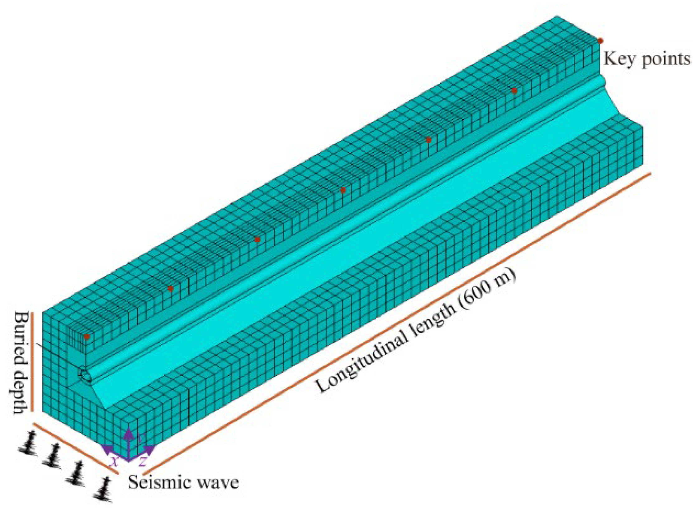
5. Numerical Simulation of Tunnels

5.1. Numerical Modeling and Parameterization

Compared with axially symmetric circular tunnels, the three-centered circular section is a more common design, especially in China’s highway tunnels and two-way high-speed rail tunnels. This study took the Ankang high-speed rail tunnel as an example to conduct seismic analysis. The tunnel is a double-track high-speed rail tunnel that adopts composite lining. The tunnel is located in the middle mountain valley area of South Qinling, where the terrain fluctuates greatly. The tectonic movement in the tunnel site area is strong and complex, with developed folds, fractures, and joint fissures. Affected by metamorphism of varying degrees, it mainly consists of phyllite and schist, and the surface is covered with Quaternary impact expansive soil, gravel soil, and a small amount of sand soil. The valleys and rivers in the tunnel site area have running water all year round, but the water volume is not large, although this is greatly affected by seasons and rainfall. During the rainy season, the water level rises and falls sharply, and the water flow is turbid. Groundwater is mainly Quaternary loose accumulation layer pore water, bedrock fissure water, and tectonic fissure water.

For further investigation, a typical section was selected as the research object to establish a numerical model of tunnel excavation and seismic dynamic response (Figure 9). The width of the model in the x direction was 100 m, the height of the model in the y direction was 100 m, and the longitudinal length of the tunnel in the z direction was set to 600 m. The tunnel section has a width of 15.1 m and a height of 12.05 m. Solid element SOLID 185 was used for surrounding rock and lining, and the constitutive behavior of geomaterial followed the Drucker–Prager criterion. The specific parameters of the surrounding rock were set as follows: density, 1950 kg/m³; modulus of elasticity, 210 MPa; and Poisson’s ratio, 0.35. Anchors were simulated by reinforcing zones, which increased the parameters of the surrounding rock by 15%. The initial support, including sprayed concrete and steel support, was simulated using shell element SHELL 181 and beam element BEAM 188, while the secondary lining was simulated using solid elements with a custom constitutive curve for concrete [22]. The artificial viscoelastic boundary parameters were A = 0.8, B = 1.1. The model contained 77,394 cells, 83,365 nodes, and the seismic wave incidence angles of the 3D model were $\alpha ={25}^{\circ }$, $\theta ={45}^{\circ }$. The model was modeled using a structured grid with a size of 5 m. The modeling was performed using a structured grid with a size of 5 m and a time step of 0.005 s.

For seismic wave selection, El Centro seismic wave data were downloaded from the PEER (Pacific Earthquake Engineering Research Center https://peer.berkeley.edu/, accessed on 1 March 2024). Seismic Data Center database, and the El Centro seismic wave acceleration is shown in Figure 10. MATLAB software was used for preprocessing, including noise removal, correction of time series, and normalization to ensure the accuracy and usability of the data. The propagation direction, frequency components, and amplitude of the seismic waves were analyzed, and the Fourier spectrum and time–frequency diagrams of the El Centro seismic waves are shown in Figure 10.

In vibration problems where damping is considered, approximations are often made using Rayleigh damping based on the assumption of linear damping [14]:

$$[C]=\alpha [M]+\beta [K],$$

(18)

where $[C],[M],[K]$ are the Rayleigh damping matrix, mass matrix, and stiffness matrix, respectively. The material damping combination coefficient, $\alpha ={\displaystyle \frac{2{\omega }_i{\omega }_j\xi }{{\omega }_i+{\omega }_j}}, \beta ={\displaystyle \frac{2\xi }{{\omega }_i+{\omega }_j}}$. ${\omega }_i,{\omega }_j$, are used to calculate the damping combination coefficient of the two frequencies, generally choose the need to cover the more concerned about the frequency band; $\xi$ is the damping ratio; according to the results of numerical calculations, the first three orders of self-oscillating frequency are: $f_1=0.69 \mathrm{Hz}$, $f_2=1.2 \mathrm{Hz}$, and $f_3=1.5 \mathrm{Hz}$. The circular frequency corresponding to the first two orders of are: ${\omega }_1=4.31 \mathrm{rad}\cdot {\mathrm{s}}^{-1}$ and ${\omega }_2=7.54 \mathrm{rad}\cdot {\mathrm{s}}^{-1}$; take the damping ratio of $\xi =5\%$, then we can obtain $\alpha =0.408, \beta =0.0217$.

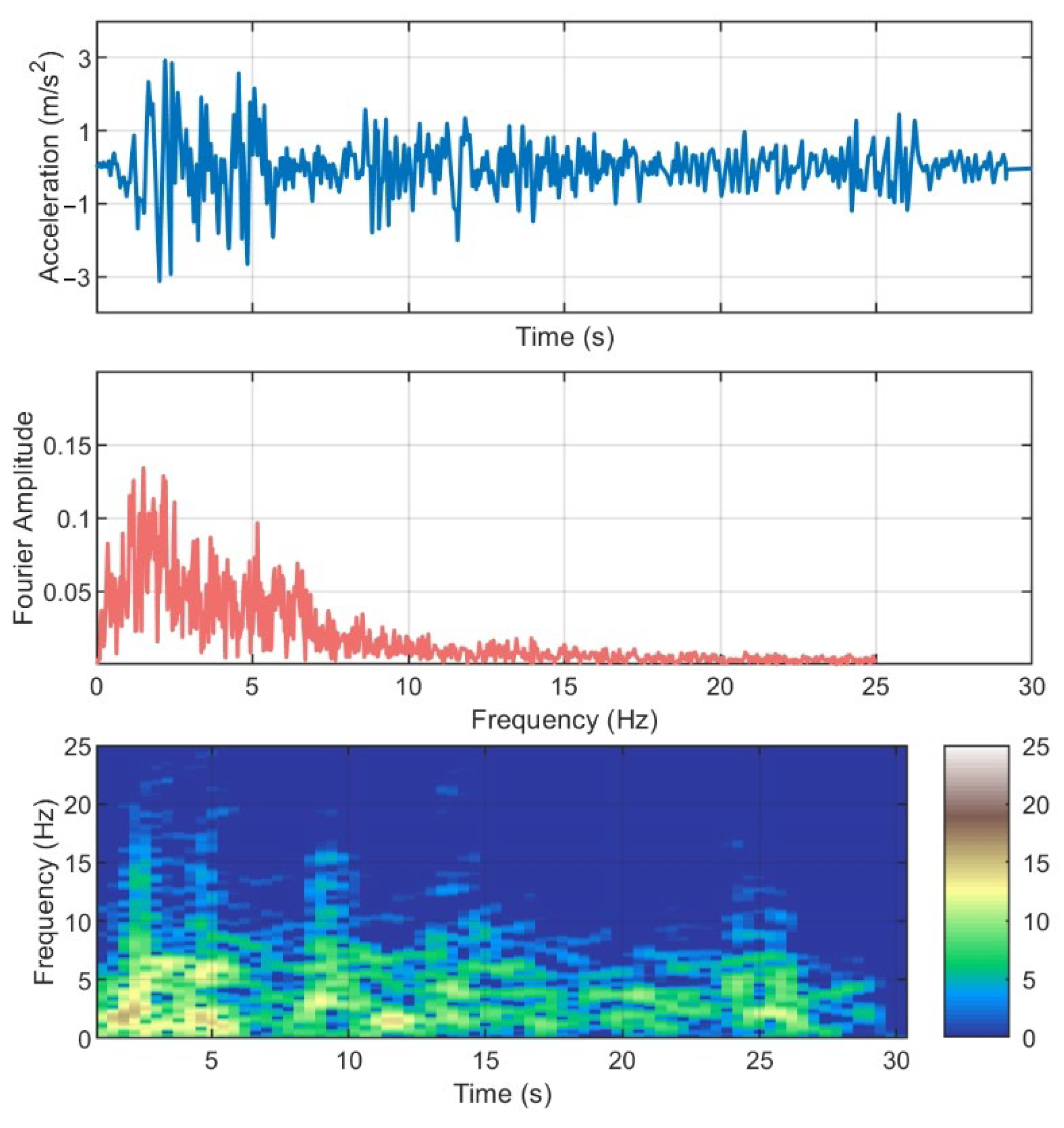
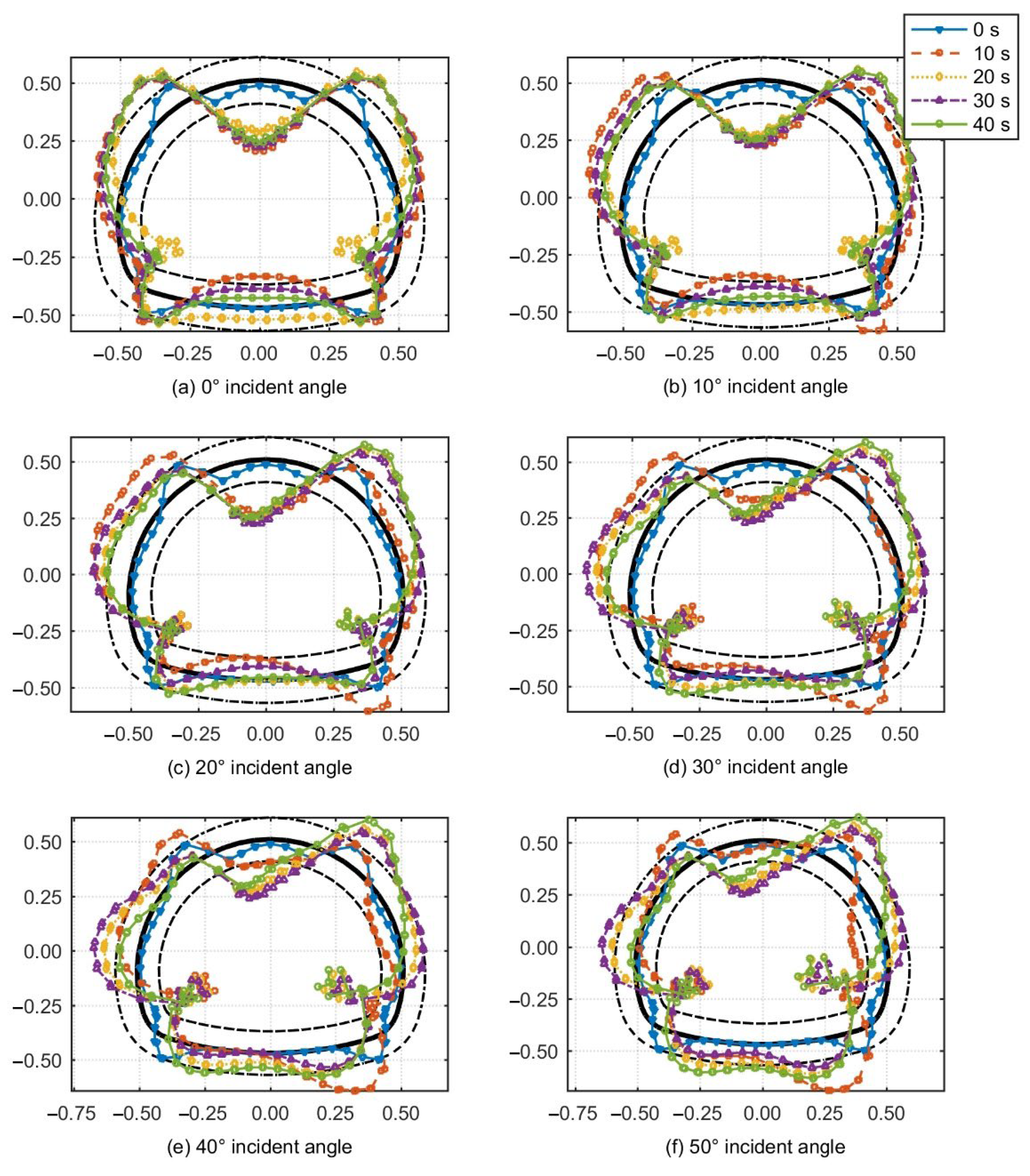
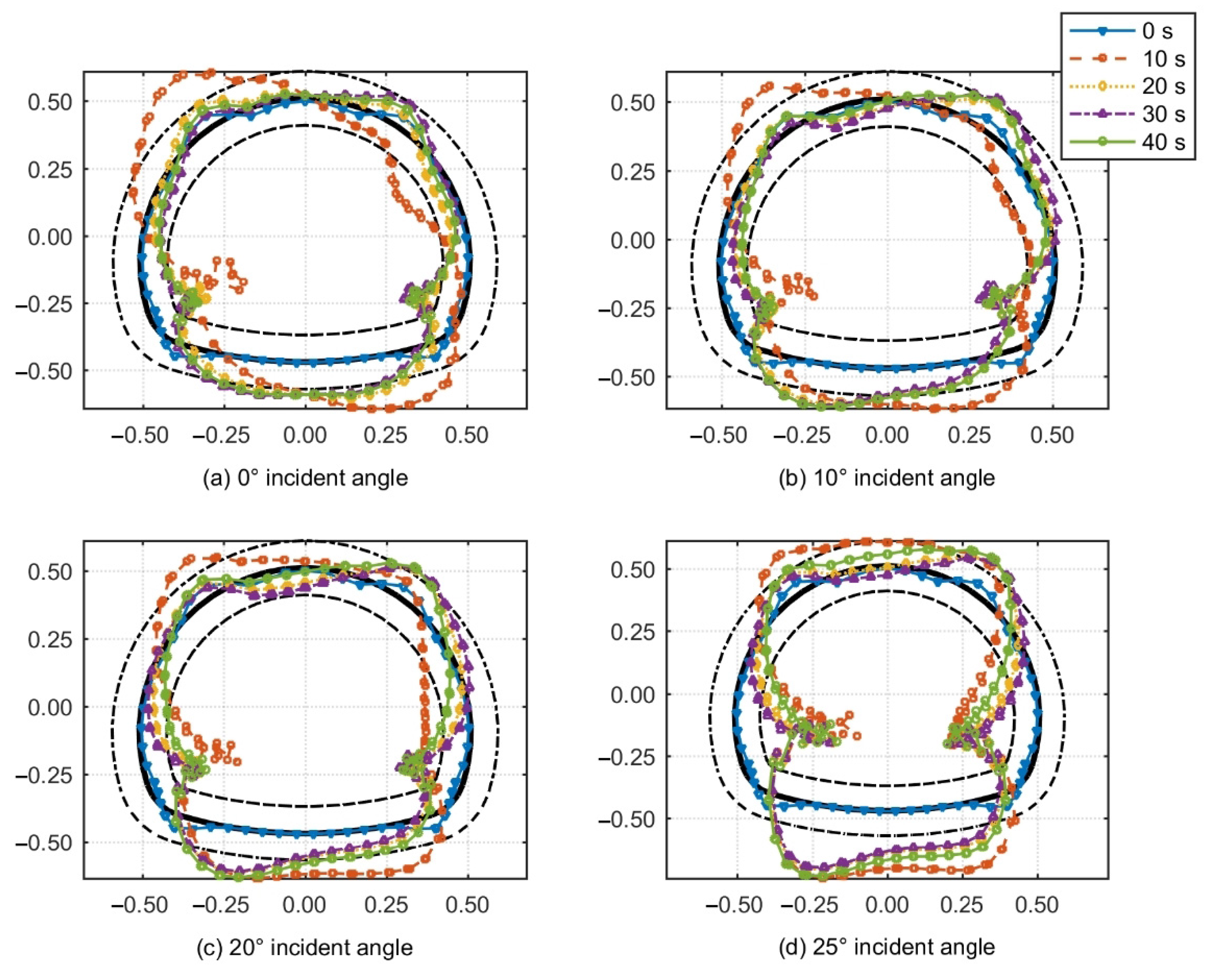
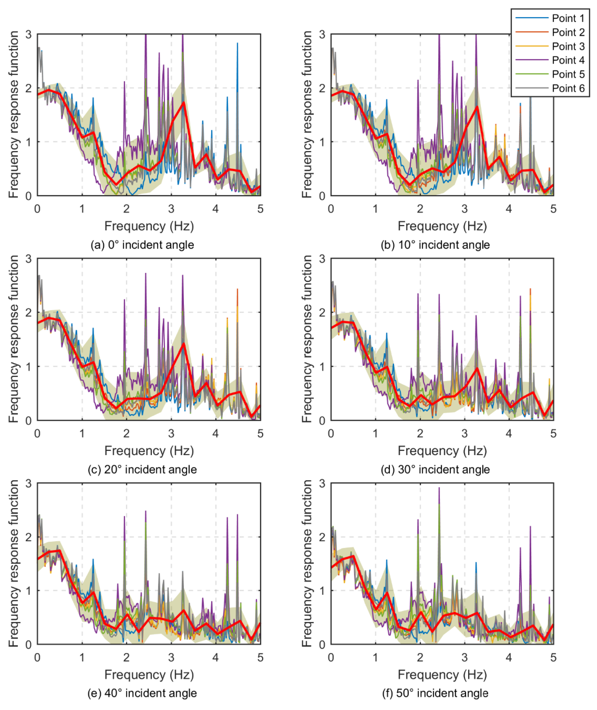
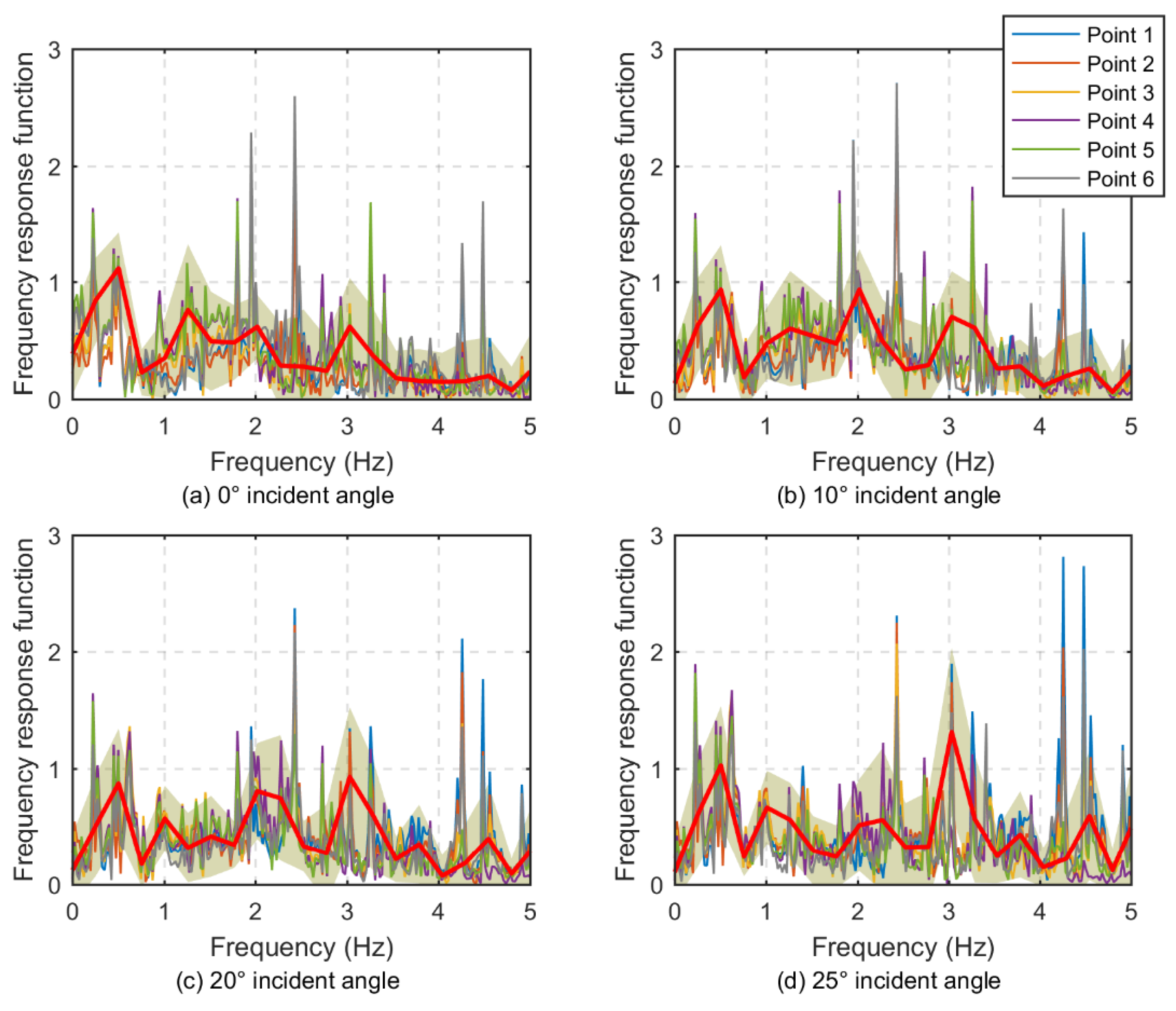
5.2. Analysis of Calculation Results

(1)

Spatial coherence factor

Seismic waves are affected by various factors such as geological conditions and topography in the process of propagation, resulting in differences in ground vibration signals at different locations. By analyzing the coherence coefficient, we can understand the change rule of seismic wave propagation in space, and then evaluate the influence of traveling wave effect on the structural response. The coherence function [33], typically denoted as $C_{xy}(\omega )$, is defined as the ratio of the product of the correlation between two signals $x(t)$ and $y(t)$ at the frequency $\omega$, and their respective power spectral densities PSD:

$$C_{ij}(\omega )={\displaystyle \frac{\left|R_{ij}(\omega )\right|}{\sqrt{S_{ii}(\omega )\cdot S_{jj}(\omega )}}},$$

(19)

where $R_{xy}(f)$ is the correlation function of the point $i, j$ at frequency $f$ and $S_{xx}(f), S_{yy}(f)$ is the power spectral density of the point $i, j$, respectively. The coherence coefficient ranges from 0 to 1, where 0 indicates that the two signals are completely uncorrelated, while 1 signifies that they are fully correlated.

Figure 11 shows the coherence coefficients of the characteristic points situated directly above the tunnel axis under the action of 3D seismic wave oblique incidence. It can be seen that the coherence coefficients exhibited the periodicity and time delay effects, and points 1 and 7 were marginally affected by the boundary effect. Notably, the coherence coefficient of the low-frequency component (exceeding 0.7) was significantly higher than that of the high-frequency component. This underscores that the oblique incidence method employed in this study predominantly reflects the time delay attributed to the traveling wave effect, whereas the stochastic excitation method excels in capturing the coherence and attenuation effects of seismic waves. When subjected to seismic wave excitation, the tunnel structure exhibited a more pronounced response compared to the surrounding ground. Wang et al. [3] have summarized four primary modes of tunnel damage observed during the Chi-Chi earthquake in Taiwan: axial stretching and compression, longitudinal bending, and ovaling. These modes provide valuable insights into the vulnerabilities of tunnel structures under seismic events. Kontoe et al. [24] posits that the ovaling of the cross-section, resulting from shear wave propagation perpendicular to the tunnel axis, constitutes a pivotal aspect. The deformation of circular tunnels and the occurrence of cyclic tensile stresses primarily affect the shoulder and knee locations. Rocking responses and ovaling deformations are characteristic of circular tunnels, whereas rectangular tunnels are more susceptible to racking distortions. Unlike circular and rectangular tunnels, three-centered circular tunnels possess flatter geometrical features, resulting in notable differences in their force characteristics. In light of this, this study concentrated on the impact of various oblique incidence angles on the ovaling distortions of three-centered circular tunnels in the planar scenario. Through an in-depth examination of how changes in the oblique incidence angle affect the ovaling trend of the tunnel structure, we aim to offer a more precise theoretical foundation and practical guidance for tunnel engineering design and construction.

(2)

Initial support moment

Under the action of seismic wave excitation, the mechanical response of a structure can usually be divided into three stages: transient, steady state, and residual. In order to explore the mechanical behavior in this process in detail, we selected five key moments, 0 s, 10 s, 20 s, 30 s, and 40 s, for observation and analysis. Figure 12 shows that the overall initial bending moment distribution of the tunnel at the initial moment (excavation static analysis) was relatively uniform, with tension on the lower side of the vault, tension on the outside of the spandrel and arch foot on both sides, and small values on the side walls and inverted arches, showing a more complex bending moment distribution than that of the circular tunnel [14]. During the seismic wave excitation (dynamic analysis), the distribution law and value of the bending moment of the primary support changed significantly, and the lateral tension of the side wall was significantly increased under the influence of the active earth pressure.

The interaction of closed forms of steady-state P, SV, and SH waves with cylindrical cavities was reported in Reference [6]. For P waves propagating perpendicular to the longitudinal axis, they proved that the peak dynamic stress concentration is about 10–15% higher than the static stress equal to the peak free-field stress. These stress concentrations were observed at wavelengths roughly 25 times the cavity diameter. Utilizing the lining stress dynamic stress concentration factor from [33], we defined the dynamic concentration factor (DCF) of the initial support bending moment as the ratio of the bending moment amplitude to the final stabilized bending moment. This ratio serves as a reliable indicator of both the pattern of ground vibration changes and the degree of stress concentration. Note, in this study, we opted not to use the static bending moment as a metric due to the involvement of tensile symbol transformations, and because the distribution of the DCF’s final bending moment bears greater similarity to the final bending moment itself. Figure 12 illustrates that the dynamic coefficient factor (DCF) of the initial bending moment of the tunnel typically remained close to 1, and with the increase of the incidence angle of the P wave, it can be observed that the bending moment of the right spandrel and arch foot was significantly larger than that of the left side, showing an asymmetrical distribution characteristic. Although the arch foot required backfilling with the inverted arch, and the bending moment at the final segment of the inverted arch was not significant, it was crucial to consider the tension on the inner side of the inverted arch during seismic excitation. The cracking of the vault lining and the inverted arch pavement demands particular attention in the case of oblique incidence of P waves. This observation aligns with the findings of post-earthquake investigations conducted on existing tunnels, as reported in reference [21].

Considering that there exists a critical angle of incidence for SV waves, beyond which total reflection occurs, as noted in reference [25]. In this study, we established four distinct SV wave incidence conditions. Figure 13 shows the change rule of the initial bending moment under SV wave incidence, in which the reference bending moment was 4 KN-m. Obviously, it can be seen that under SV wave excitation, the initial bending moment was significantly affected by the shear effect, and its bending moment changed much more than that of P wave incidence [4]. Specifically, under SV wave excitation, the initial bending moment experienced a notable impact from the shear effect, leading to a substantially larger magnitude of bending moment variation than that observed during P wave incidence. When SV waves were incident vertically, the initial bending moment of the tunnel manifested as ovaling. This was evident in the conspicuous straining of the left arch shoulder and the outer portion of the right arch foot, whereas the right arch shoulder and the inner part of the left arch foot exhibited strain as well. Following the cessation of the seismic wave, the steady-state tends to exhibit symmetrical stress distribution. In comparison to the static state, the side wall and the uplift arch emerged as critical areas deserving special attention. Taking into account the back-filling of the inverted arch and the stress concentration at the junction of the side wall and footing, it was observed that the tension on the exterior of the up-arch did not induce excessive damage. As the SV wave incidence angle increased, the tensile state of the inner side of the side wall became progressively more pronounced, concomitant with a significant rise in tension on the outer side of the inverted arch. Overall, the vertical incidence of SV led to the deformation of the tunnel structure with ovaling deformation, and subsequently led to substantial shear deformation in the arch shoulder segment of the primary support. Furthermore, as the oblique incidence angle augmented, the vulnerable sections of the lining shifted towards the side wall and the arch foot.

(3)

Lining Fourier spectrum

The maximum acceleration and frequency components for typical monitoring points of the lining were documented for the scenario of vertical incidence of P waves, as detailed in

Table 1. Lining accelerations of the Ankang tunnel for P waves incident vertically.

Monitoring Station	Max Accel. (m/s)2	Largest Peak Accel. (m/s)2	Freq. (Hz)	2nd Peak Accel. (m/s)2	Freq. (Hz)	3rd Peak Accel. (m/s)2	Freq. (Hz)
Excitation acceleration	1.826	0.113	1.175	0.089	1.500	0.088	2.150
Vault	1.826	0.137	1.177	0.127	0.852	0.126	0.351
Left arch shoulder	1.926	0.125	0.351	0.119	0.852	0.117	0.376
Left arch footing	1.971	0.124	0.351	0.116	0.376	0.115	0.852
Inverted arch	2.598	0.127	2.154	0.122	0.351	0.113	0.376
Right arch shoulder	1.984	0.124	0.351	0.116	0.376	0.114	0.852
Right arch footing	1.927	0.125	0.351	0.119	0.852	0.117	0.376

. Upon analyzing the Fourier spectrum, it was evident that the primary frequency peaks of acceleration at various lining sections were comparable, falling within the 0.10–0.14 range. Notably, the first principal frequency for the left and right arch shoulders and sidewalls was approximately 0.35 Hz, whereas the vault and inverted arch differed, with frequencies of 1.18 Hz and 2.15 Hz, respectively. Actual tunnel monitoring data reveals that the ratio of the tunnel structure’s first principal frequency under seismic excitation to that of seismic monitoring stations lies between approximately 1/17 and 1/2.5 [4]. The maximum acceleration magnitude recorded for the superelevation arch was 2.60 m/s², which further confirms that the possible damage of the roadway cracking due to inverted arch stress during the vertical incidence of the P wave is an urgent concern for the lining structure.

Table 2. Lining accelerations of the Ankang tunnel for SV waves incident vertically.

Monitoring Station	Max Accel. (m/s)2	Largest Peak Accel. (m/s)2	Freq. (Hz)	2nd Peak Accel. (m/s)2	Freq. (Hz)	3rd Peak Accel. (m/s)2	Freq. (Hz)
Excitation acceleration	1.826	0.113	1.175	0.089	1.500	0.088	2.150
Vault	0.987	0.044	1.779	0.042	2.079	0.042	2.204
Left arch shoulder	0.830	0.036	1.779	0.033	1.578	0.031	1.503
Left arch footing	1.056	0.054	1.503	0.048	1.779	0.047	1.177
Inverted arch	1.337	0.072	1.503	0.063	1.177	0.063	1.779
Right arch shoulder	1.372	0.074	1.503	0.069	1.779	0.060	1.578
Right arch footing	1.219	0.060	2.204	0.059	2.154	0.059	1.779

outlines the structural response of the tunnel during vertical SV wave incidence, exhibiting patterns distinct from those observed under P wave incidence. With SV waves, the peak principal frequencies for the arch, arch shoulder, and footing predominantly fell within the 1.5–1.8 Hz range, while the superelevation arch slightly exceeded this at 2.2 Hz. In contrast to P waves, the acceleration peaks in these regions were lower, ranging only from 0.03–0.08. In addition, the peak acceleration was notably higher on the right arch shoulder footing and inverted arch compared to the left side. In summary, the tunnel structure experienced shear forces, leading to ovaling deformation at the right arch shoulder and left arch footing. The first principal frequencies of the tunnel structure under SV waves were more uniform, potentially elevating the risk of resonance-induced damage to the structure.

(4)

Lining frequency response function

The transfer function (frequency response function), which responds to the frequency–domain relationship between the inputs and outputs of a system, reflects the inherent characteristics of the system and is usually expressed as:

$$H(s)=Y(s)/X(s),$$

(20)

where $H(s)$ is the transfer function and $X(s), Y(s)$ is the Laplace transform of the input and output, respectively.

Recent studies [3] have consistently demonstrated that tunnel depth and seismic wavelength exert a profound influence on the mechanical response of tunnels. Specifically, when the wavelength of the surrounding rock reaches one-quarter of the tunnel depth, the amplification effect becomes particularly pronounced. Furthermore, shallow tunnels exhibit a more potent amplification effect compared to deep tunnels, especially at low frequencies [4]. Six typical characteristic points of the lining site were selected to explore the frequency response function curves of the lining displacement. The frequency response function was normalized according to the amplitude in the frequency range of 0–5 Hz, as shown in Figure 14. Under the influence of vertical incidence of P waves, the lining structure experienced a drastic overall response near 0.3 Hz and 3.0 Hz. The maximum value of the transfer coefficient exceeded three, with notable variations observed in different parts of the structure. For instance, the resonance frequency of the elevated arch was approximately 2.2 Hz (Table 1), resulting in a significant amplification effect. As the incident angle increased, the response of the lining structure became concentrated below 2.0 Hz, and the bandwidth gradually narrowed. When the seismic frequency exceeded 2.0 Hz, the attenuation of the seismic wave signal became evident. This attenuation exhibited frequency dependence, with high-frequency components being more readily absorbed than low-frequency components. Consequently, the amplitude of the high-frequency components of the waveform decreased more rapidly. However, it is also possible that this phenomenon arises from the artificial damping or filtering effect introduced by the numerical model. Specifically, the numerical integration and differentiation algorithm can act as a high-pass filter, and a higher sampling frequency may lead to more severe high-frequency noise and larger errors in the calculated acceleration. In contrast, the SV wave incidence case showed a multi-frequency response with more homogenized characteristics. As shown in Figure 15, the frequency response transfer drastic were mainly distributed in the 0–4.0 Hz range, and different parts of the frequency response frequency were also closer.

(5)

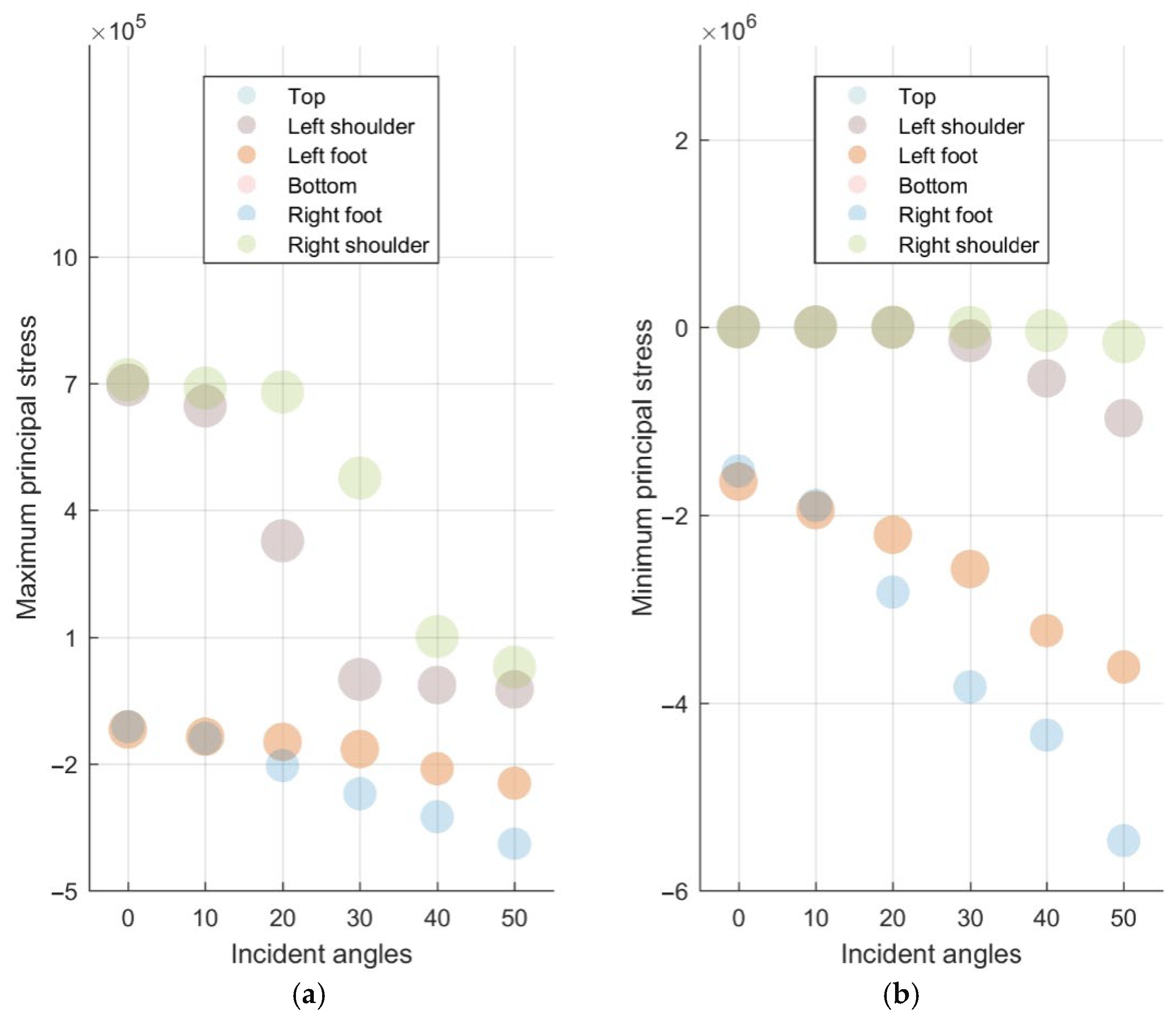
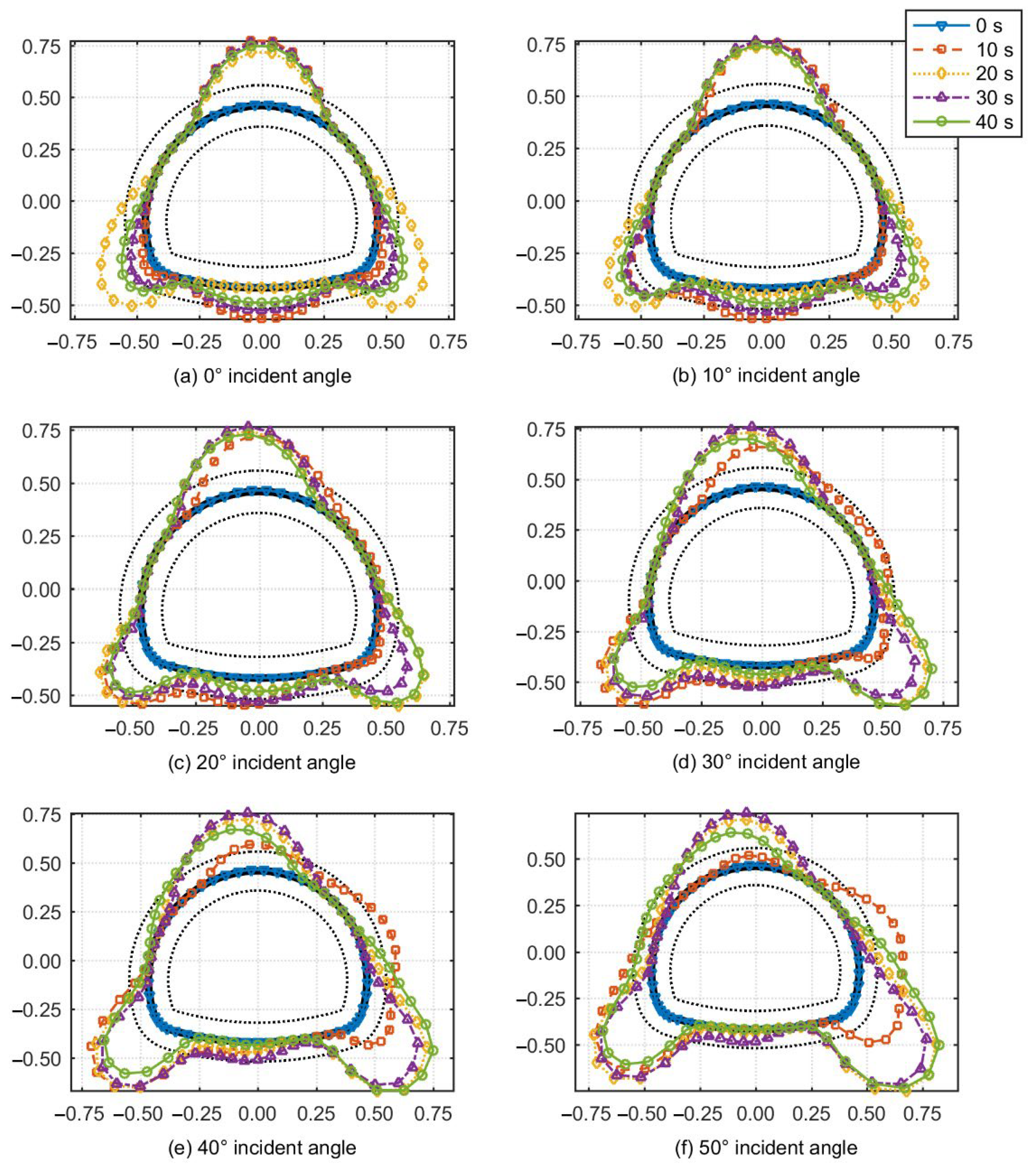
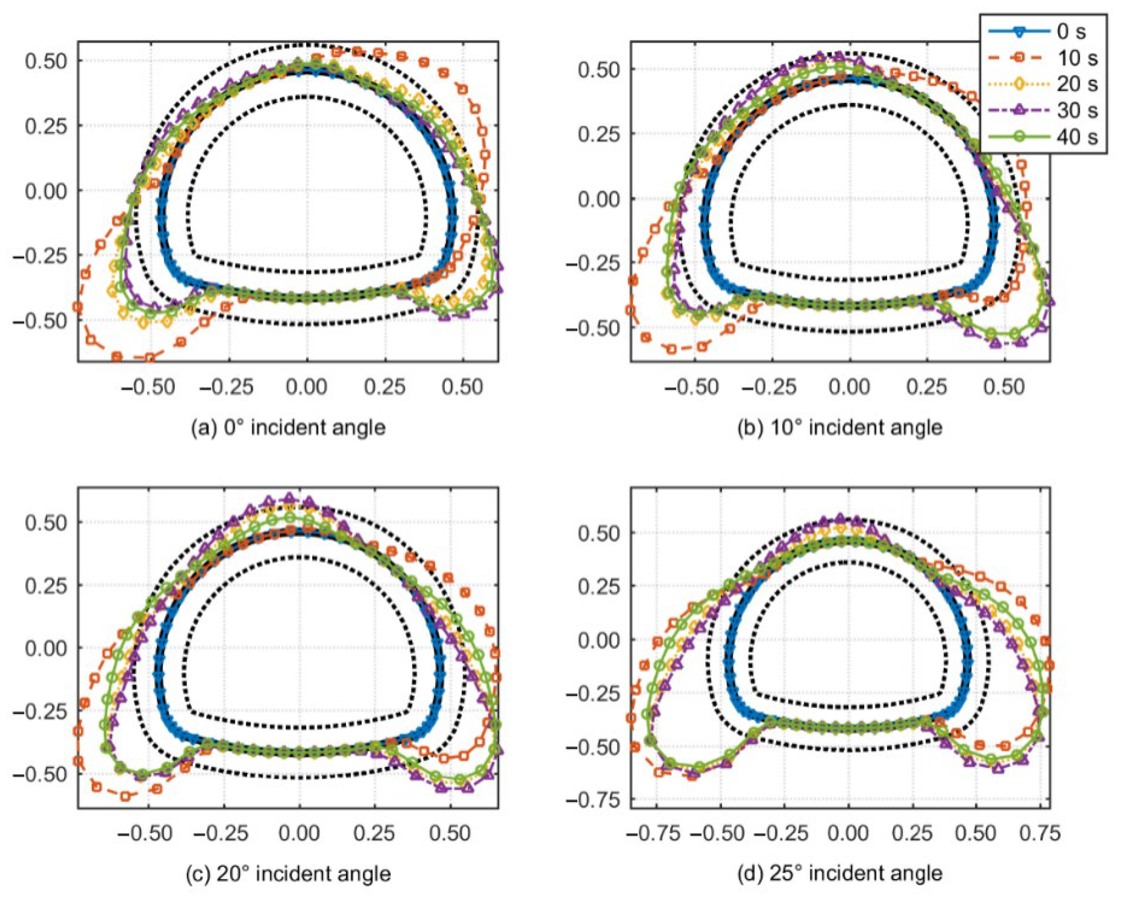
Lining principal stresses

Wang et al. [3] employed the “flexibility ratio” to quantify the relative stiffness between the lining and the surrounding soil, thereby characterizing the tunnel structure’s capacity to resist ground deformation.

$$F={\displaystyle \frac{E_m(1-{\mu }_t^2)R^3}{6E_{t}I(1+{\mu }_m)}}\approx 68,$$

(21)

where $E_m$${\mu }_m$$E_t$${\mu }_t$ denotes the modulus of elasticity and Poisson’s ratio of the foundation and structure, respectively; $R$ is the radius of the tunnel; and $I$ is the moment of inertia of the tunnel section. The $E_t$ was adjusted to investigate the effect of different flexibility ratios. Several researchers have explored the correlation between the flexibility ratio and the degree to which the lining modifies the tunnel’s response to static or dynamic loads. They have concluded that a flexibility ratio exceeding 20 denotes a lining with full flexibility [4]. In such scenarios, the lining will accommodate the deformation imposed by the surrounding medium. Conversely, when the flexibility ratio is low, the lining will resist the deformation (distortion) induced by the medium. Figure 16 illustrates the variation in stress at characteristic points of the lining in relation to the P wave incidence angle. It was observed that as the angle of oblique incidence increases, the maximum principal stress across various segments of the lining diminished to varying extents, with the most significant reduction observed at the arch shoulders. However, the order of magnitude of this stress reduction was not substantial, and thus, it is unlikely to induce tensile cracking in the concrete. In contrast, the trend for the maximum compressive stress indicates a general increase.

Upon an increase in the P wave incidence angle, the compressive stress at the left and right arch footings exhibited a sharp rise, whereas the remaining sections of the arch experienced an increase as well, albeit relatively minor. The horizontal displacement of the lining structure was positive for the left arch shoulder and footing, with the rest of the sections registering negative displacement, characterized by a slight variation in value. Figure 17 elucidates the stress variation at characteristic points of the lining as a function of the SV wave incidence angle. It is apparent that with incremental increases in the oblique incidence angle, the maximum principal stress at the left and right arches and feet of the lining was significantly diminished, while the stress at the other positions remained largely unaltered. However, the trend for the maximum compressive stress was converse; as the SV wave incidence angle increased, the compressive stress at the left and right footings spiked sharply, with the maximum value approaching 10 MPa. The remaining sections also exhibited an increase, though this was less pronounced. Regarding the horizontal displacement of the lining structure, the right arch shoulder and foot displayed negative displacement, while the other parts were positive. The magnitude of horizontal displacement remained largely stable, with the right arch foot exhibiting the most significant reduction.

Results from physical modeling tests conducted with a shaking table and a centrifuge indicate that under seismic excitation, the tunnel responds with vibratory motion characterized by elliptical deformation or tilting and twisting. Following vibration, there was residual earth pressure exerted on the sidewalls of the tunnel, and the internal forces within the lining persisted [6]. The initial support served as a temporary structural support during construction, whereas the forces and deformations of the secondary lining warrant greater attention. This study simulated the excavation and support process, and the calculated results for the secondary lining were notably lower compared to the load structure method.

Figure 18 depicts the maximum compressive stress within the lining structure during P wave incidence. With respect to stress distribution characteristics, the crown of the arch and the regions adjacent to the footings warrant particular consideration. As the angle of P-wave incidence increases, there is a slight decrement in compressive stress at the arch crown, concomitant with a slight increment in the compressive stress within the arch footings. Overall, when P-waves impinge perpendicularly, the stress magnitudes within the lining are relatively modest. However, as the angle of oblique incidence escalates, the “rotational effect” exerts a more pronounced influence, leading to a substantial amplification in both the areas of stress concentration and their respective magnitudes. Figure 19 illustrates the maximum compressive stress. During vertical incidence, the maximum compressive stress was concentrated in the right shoulder and the right footing. Subsequently, the maximum compressive stress shifted to the right arch shoulder and left arch foot, with values approaching 10 MPa. However, as the incidence angle increased, the “rotational effect” caused the maximum compressive stress to migrate towards the left and right sidewalls [34,35]. In summary, the lining stress induced by the SV wave was markedly greater than that induced by the P wave of the same amplitude when incident vertically. With the increase of the incidence angle, the stress distribution area underwent rotation, although the magnitude of the stress value change was relatively modest.

6. Conclusions

Generally, tunnels and underground structures exhibit robust seismic performance. However, since the Hanshin earthquake in Japan, the Chi-Chi earthquake in Taiwan, and the Wenchuan earthquake, there has been an increase in seismic events affecting tunnels, leading to significant structural damage and drawing increasing attention from the underground engineering community. Initially, this study analyzed the reflection characteristics of elastic P waves incident upon a free plane, encompassing the evolutionary laws of the reflection angle, as well as the amplitude and phase of the reflected P wave and SV wave.

Based on this foundation, the matrix analysis method for calculating the equivalent nodal loads under artificial truncated boundary conditions for seismic wave oblique incidence was established by utilizing coordinate transformation technology, considering the displacement velocity and stress characteristics of plane waves. The proposed artificial boundary conditions were expanded for the simulation of static excavation and dynamic coupling analysis of tunnels using birth–death element technology, and further developed into a three-dimensional seismic oblique incidence model. Ultimately, the spatial non-uniformity of ground vibration and the dynamic response of the surrounding rock for various seismic wave oblique incidence angles were analyzed. The nonlinear response of the tunnel structure to different seismic wave oblique incidence angles was investigated, along with the spectral correlation of the seismic dynamic response of the tunnel structure. The research findings indicate the following:

(1)

The oblique incidence method effectively captures the traveling wave effect, whereas the attenuation and coherence effects are partially dependent on the random excitation method. In the analysis of P wave and SV wave incidence, the “rotation effect” due to oblique incidence must be accounted for, as it significantly influences the stress and deformation of the tunnel structure, exhibiting distinct rotational characteristics for different wave types.

(2)

During P wave incidence, particular attention should be given to the structural safety of the vault and the haunch due to the impact of extension waves. As the oblique incidence angle increases, the structural forces and deformations rotate to a certain extent, with a marked increase in relevant values, posing a potential threat to the stability of the tunnel structure.

(3)

Under the shear action of SV waves, the tunnel structure may undergo ovaling deformation, rendering the arch shoulders and side walls more susceptible to damage. As the angle of oblique incidence rises, the hazardous areas are shifted to the crown and inverted arch by the “rotation effect,” although the changes in the relevant values are not pronounced.

(4)

Compared to tunnels with a circular cross-section, the low-frequency amplification of seismic waves in the surrounding rock and the variability of the frequency response function across different lining sections are more pronounced. Notably, the dominant frequency characteristics are very significant during P wave incidence; with the increase in the incidence angle, the attenuation of the seismic wave signal becomes more apparent. In contrast, the SV wave exhibits a more uniform behavior. These insights are of paramount importance for enhancing the understanding and refinement of the seismic design of tunnels and underground structures.

References

1. Du, X.L.; Li, Y.; Xu, C.S.; Lu, D.C.; Xu, Z.G.; Jin, L. Review on damage causes and disaster mechanism of Daikai subway station during 1995 Osaka-Kobe Earthquake. Chin. J. Geotech. Eng. 2018, 40, 223–236. [Google Scholar]
2. Yan, K.; Zhang, J.; Wang, Z.; Liao, W.; Wu, Z. Seismic responses of deep buried pipeline under non-uniform excitations from large scale shaking table test. Soil Dyn. Earthq. Eng. 2018, 113, 180–192. [Google Scholar]
3. Wang, W.; Wang, T.; Su, J.; Lin, C.; Seng, C.; Huang, T. Assessment of damage in mountain tunnels due to the Taiwan Chi-Chi Earthquake. Tunn. Undergr. Space Technol. 2001, 16, 133–150. [Google Scholar]
4. Wang, T.; Kwok, O.A.; Jeng, F. Seismic response of tunnels revealed in two decades following the 1999 Chi-Chi earthquake (Mw 7.6) in Taiwan: A review. Eng. Geol. 2021, 287, 106090. [Google Scholar]
5. Wang, W.L.; Su, Z.J.; Lin, J.H.; Cheng, J.R.; Wang, T.D.; Wang, C.H. Discussion on damaged extent of mountainous tunnels due to earthquake, Taiwan. Mod. Tunn. Technol. 2001, 02, 52–60. [Google Scholar]
6. St John, C.M.; Zahrah, T.F. Aseismic design of underground structures. Tunn. Undergr. Space Technol. 1987, 2, 165–197. [Google Scholar]
7. Penzien, J. Seismically induced racking of tunnel linings. Earthq. Eng. Struct. Dyn. 2000, 29, 683–691. [Google Scholar]
8. Zhu, J.; Li, X.J.; Liang, J.W. Seismic responses of underground tunnels subjected to obliquely incident seismic waves by 2.5D FE-BE coupling method. Chin. J. Geotech. Eng. 2022, 44, 1846–1854. [Google Scholar]
9. Huang, W.Z.; He, C.; Xu, G.Y.; Li, B. Seismic response of a submarine immersed tunnel under oblique incidence of SV waves. Tunnel Constr. 2024, 44, 724. [Google Scholar]
10. Hashash, Y.M.A.; Tseng, W.S.; Krimotat, A. Seismic Soil-Structure Interaction Analysis for Immersed Tube Tunnels Retrofit. In Geotechnical Earthquake Engineering and Soil Dynamics III. Geotech. Spec. Publ. 1998, 75, 1380–1391. [Google Scholar]
11. Hwang, J.H.; Lu, C.C. Seismic capacity assessment of old Sanyi railway tunnels. Tunn. Undergr. Space Technol. 2007, 22, 433–449. [Google Scholar]
12. Yu, H.B.; Yang, Y.S.; Yuan, Y.; Duan, K.P.; Gu, Q. A comparison between vibration and wave methods in seismic analysis of underground structures. Earthq. Eng. J. 2019, 41, 845–852. [Google Scholar]
13. Ding, Z.D.; Chen, Y.S.; Zi, H. Study on artificial boundary and ground motion input method in tunnel seismic response. Earthq. Eng. Eng. Dyn. 2022, 42, 52–61. [Google Scholar]
14. Yan, L.; Haider, A.; Li, P.; Song, E. A numerical study on the transverse seismic response of lined circular tunnels under obliquely incident asynchronous P and SV waves. Tunn. Undergr. Space Technol. 2020, 97, 103235. [Google Scholar]
15. Zhu, S.; Li, W.H.; Lee, V.W.; Zhao, C. Analytical solution of seismic response of an undersea cavity under incident P1-wave. Rock Soil Mech. 2021, 42, 93–103. [Google Scholar]
16. Zhu, J.; Li, X.J.; Liang, J.W.; Bin, Z. Effects of a tunnel on site ground motion for 3D obliquely incident seismic waves. China Civil Eng. J. 2020, 53, 318–324. [Google Scholar]
17. Du, X.L.; Xu, Z.G.; Xu, C.S.; Li, Y.; Jiang, J.W. Time-history analysis method for soil-underground structure system based on equivalent linear method. Chin. J. Geotech. Eng. 2018, 40, 2155–2163. [Google Scholar]
18. Liu, J.B.; Bao, X.; Tan, H.; Wang, D.Y.; Li, S.T. Seismic wave input method for soil-structure dynamic interaction analysis based on internal substructure. China Civil Eng. J. 2020, 53, 1–8. [Google Scholar]
19. Zhang, D.D.; Liu, Y.; Xiong, F.; Mei, Z. Seismic response analysis of rock tunnel near-portals under oblique incidence of P-wave and SV-wave. Shock Vib. 2022, 41, 278–286. [Google Scholar]
20. Song, Z.; Wang, F.; Li, Y.; Liu, Y. Nonlinear seismic responses of the powerhouse of a hydropower station under near-fault plane P-wave oblique incidence. Eng. Struct. 2019, 199, 109613. [Google Scholar]
21. Chen, D.; Pan, Z.; Zhao, Y. Seismic damage characteristics of high arch dams under oblique incidence of SV waves. Eng. Fail. Anal. 2023, 152, 107445. [Google Scholar]
22. Huang, J.-Q.; Du, X.-L.; Zhao, M.; Zhao, X. Impact of incident angles of earthquake shear (S) waves on 3-D non-linear seismic responses of long lined tunnels. Eng. Geol. 2017, 222, 168–185. [Google Scholar]
23. Zhang, W.; Seylabi, E.E.; Taciroglu, E. An ABAQUS toolbox for soil-structure interaction analysis. Comput. Geotech. 2019, 114, 103143. [Google Scholar]
24. Kontoe, S.; Zdravkovic, L.; Potts, D.M.; Menkiti, C.O. Case study on seismic tunnel response. Can. Geotech. J. 2008, 45, 1743–1764. [Google Scholar]
25. Aki, K.; Richards, P.G. Quantitative Seismology: Theory and Methods; University Science Books: Sausalito, CA, USA, 1980; pp. 204–356. [Google Scholar]
26. Babich, V.; Kiselev, A. Elastic Waves; Taylor and Francis: Washington DC, USA, 2018; pp. 1–65. [Google Scholar]
27. Pujol, J. Elastic Wave Propagation and Generation in Seismology; Cambridge University Press: Cambridge, UK, 2003; pp. 112–193. [Google Scholar]
28. Landau, L.D.; Lifshitz, E.M. Theory of Elasticity, 3rd ed.; Pergamon Press: Oxford, UK, 1986; pp. 21–87. [Google Scholar]
29. Ma, S.J.; Chi, M.J.; Chen, X.L.; Chen, S.; Chen, H.J.; Xing, H.J. Research on the static-dynamic boundary switch and its rationality verification method. Acta Seismol. Sinica 2024, 46, 157–171. [Google Scholar]
30. Liu, J.; Wang, Z.; Du, X.; Du, Y.-X. Three dimensional viscous-spring artificial boundaries in time domain for wave motion problems. Eng. Mech. 2005, 22, 46–51. [Google Scholar]
31. Gao, F.; Zhao, Z.B. Study on transformation method for artificial boundaries in static-dynamic analysis of underground structure. J. Vib. Shock 2011, 30, 165–170. [Google Scholar]
32. Su, W.; Qiu, Y.-X.; Xu, Y.-J.; Wang, J.-T. A scheme for switching boundary condition types in the integral static-dynamic analysis of soil-structures in Abaqus. Soil Dyn. Earthq. Eng. 2021, 141, 106458. [Google Scholar]
33. Zhou, Y.Q.; Sheng, Q.; Li, N.N.; Fu, X.D. Preliminary study on time-space effect of the dynamic response of long tunnel under non-uniform ground motion. Rock Soil Mech. 2021, 11, 2287–2297. [Google Scholar]
34. Hashash, Y.M.A.; Hook, J.J.; Schmidt, B.; Yao, I.C. Seismic design and analysis of underground structures. Tunn. Undergr. Space Technol. 2001, 16, 247–293. [Google Scholar]
35. Shen, Y.; Gao, B.; Yang, X.; Tao, S. Seismic damage mechanism and dynamic deformation characteristic analysis of mountain tunnel after Wenchuan earthquake. Eng. Geol. 2014, 180, 85–98. [Google Scholar]
Figure 1. Schematic illustration of 3D oblique seismic wave incidence.
Buildings 14 02940 g001
Figure 2. Reflection coefficients of plane wave incident on the free surface.
Buildings 14 02940 g002
Figure 3. Schematic diagram of equivalent nodal load calculation. (a) Nodal distribution with artificially truncated boundary, scattered field inside and free field outside. (b) Schematic of equivalent node load calculation with nodal hydrostatic fixed boundary. (c) Nodal statics fixed boundary converted to dynamics artificial boundary conditions. (d) Equivalent nodal load calculation with nodal dynamics artificial boundary.
Buildings 14 02940 g003
Figure 4. Displacement law under the incidence of P wave for 0.4 s (a), 0.8 s (b), 1.2 s (c), and 1.6 s (d).
Buildings 14 02940 g004
Figure 5. Displacement law under the incidence of SV wave for 0.4 s (a), 0.8 s (b), 1.2 s (c), and 1.6 s (d).
Buildings 14 02940 g005
Figure 6. Displacements for the characteristic point of soil under the SV wave.
Buildings 14 02940 g006
Figure 7. Displacement law under the incidence of P and SV waves.
Buildings 14 02940 g007
Figure 8. The displacements of the soil resulting from P wave incidence.
Buildings 14 02940 g008
Figure 9. Schematic diagram of tunnel finite element model.
Buildings 14 02940 g009
Figure 10. El Centro seismic wave acceleration, Fourier spectrum, and time–frequency plots.
Buildings 14 02940 g010
Figure 11. The coherence coefficients at seven points on the ground above the tunnel axis.
Buildings 14 02940 g011
Figure 12. The initial bending moment with time for different P wave incidence angles. The thick black solid line represents the tunnel outline. The inner black dashed line (positive values) indicates the bending moment, while the outer black dotted line (negative values) represents the bending moment characteristic values (2.0 KN-m).
Buildings 14 02940 g012
Figure 13. Distribution pattern of initial bending moments for different SV incidence angles. The thick black solid line represents the tunnel outline. The inner black dashed line (positive values) indicates the bending moment, while the outer black dotted line (negative values) represents the bending moment characteristic values (4.0 KN-m).
Buildings 14 02940 g013
Figure 14. Frequency response functions of the lining structure at different angles of incidence of the P waves.
Buildings 14 02940 g014
Figure 15. Frequency response functions of the lining structure at different angles of incidence of the SV waves.
Buildings 14 02940 g015
Figure 16. (a) Maximum principal stresses and (b) minimum principal stresses in the two-lined feature sites at different P wave incidence angles. Since the tunnel has a symmetrical structure, the final stress values of the left and right arch shoulders (foot) are identical, leading to overlapping labels in the figure.
Buildings 14 02940 g016
Figure 17. (a) Maximum principal stresses and (b) minimum principal stresses in the two-lined feature sites at different SV wave incidence angles. Since the tunnel has a symmetrical structure, the final stress values of the left and right arch shoulders (foot) are identical, leading to overlapping labels in the figure.
Buildings 14 02940 g017
Figure 18. Maximum compressive stress of the second lining under different P wave incidence angles. The thick black solid line represents the tunnel outline. The inner black dashed line (positive values) indicates the bending moment, while the outer black dotted line (negative values) represents the stress characteristic values (1.0 MPa).
Buildings 14 02940 g018
Figure 19. Maximum compressive stress of the second lining under different SV wave incidence angles. The thick black solid line represents the tunnel outline. The inner black dashed line (positive values) indicates the bending moment, while the outer black dotted line (negative values) represents the stress characteristic values (2.0 MPa).
Buildings 14 02940 g019