Physically Guided Estimation of Vehicle Loading-Induced Low-Frequency Bridge Responses with BP-ANN

Abstract

The intersectional relationship in bridge health monitoring refers to the mapping function that correlates bridge responses across different locations. This relationship is pivotal for estimating structural responses, which are then instrumental in assessing a bridge’s service status and identifying potential damage. The current research landscape is heavily focused on high-frequency responses, especially those associated with single-mode vibration. When it comes to low-frequency responses triggered by multi-mode vehicle loading, a prevalent strategy is to regard these low-frequency responses as “quasi-static” and subsequently apply time-series prediction techniques to simulate the intersectional relationship. However, these methods are contingent upon data regarding external loading, such as traffic conditions and air temperatures. This necessitates the collection of long-term monitoring data to account for fluctuations in traffic and temperature, a task that can be quite daunting in real-world engineering contexts. To address this challenge, our study shifts the analytical perspective from a static analysis to a dynamic analysis. By delving into the physical features of bridge responses of the vehicle–bridge interaction (VBI) system, we identify that the intersectional relationship should be inherently time-independent. The perceived time lag in quasi-static responses is, in essence, a result of low-frequency vibrations that are aligned with driving force modes. We specifically derive the intersectional relationship for low-frequency bridge responses within the VBI system and determine it to be a time-invariant transfer matrix associated with multiple mode shapes. Drawing on these physical insights, we adopt a time-independent machine learning method, the backpropagation–artificial neural network (BP-ANN), to simulate the intersectional relationship. To train the network, monitoring data from various cross-sections were input, with the responses at a particular section designated as the output. The trained network is now capable of estimating responses even in scenarios where time-related traffic conditions and temperatures deviate from those present in the training data set. To substantiate the time-independent nature of the derived intersectional relationship, finite element models were developed. The proposed method was further validated through the in-field monitoring of a continuous highway bridge. We anticipate that this method will be highly effective in estimating low-frequency responses under a variety of unknown traffic and air temperature conditions, offering significant convenience for practical engineering applications.

1. Introduction

Simulating an intersectional relationship is a key area of focus in bridge health monitoring. By utilizing historical monitoring data from multiple cross-sections, it is possible to model the intersectional relationship [1] that exists between these locations. This model can then be used to estimate the current response at a specific cross-section by multiplying the relationship with the responses recorded at other cross-sections. If there is a significant discrepancy between the actual current monitoring data and the estimated results, it could be an indication of potential damage in the vicinity of that particular cross-section. This approach provides a valuable tool for identifying structural issues and ensuring the ongoing safety and integrity of a bridge.

The majority of the current research concentrates on the intersectional relationship associated with high-frequency responses [2], with scant attention given to low-frequency responses. It has been demonstrated that the intersectional relationship acts as a transfer matrix determined by mode shapes. Consequently, it is essential to initially identify a bridge’s mode shapes. Subsequently, several explicit mode shape identification methods may become available, such as Stochastic Subspace Identification (SSI) [3,4], Independent Component Analysis (ICA) [5,6], and other general physical parameter-identification methods [7,8,9]. With these methods, the intersectional relationship can be further estimated. However, for typical low-frequency responses induced via vehicle loading, the corresponding frequencies not only are low but also vary with a vehicle’s moving speed. Moreover, the differences between these frequencies are minimal, making it challenging to identify bridge-mode shapes using most of the aforementioned methods [10,11].

In place of the term for “low-frequency” responses, existing research often employs the descriptor of “quasi-static” responses [12,13] to circumvent the challenges associated with identifying bridge-mode shapes. From a static structural analysis perspective, quasi-static responses are considered to be time-dependent functions. According to the conventional static deflection calculation method, such as the influence line [14], the vertical displacement time–history curve should trace a piecewise cubic function, with inflection points occurring at the moments when a vehicle passes over the observed cross-section. Moreover, the timing of the maximum displacement correlates with the vehicle’s travel speed, as well as its entry and exit times. Specifically, a temporal lag [15] is observed between the quasi-static displacement time histories at different cross-sections. Consequently, it has been assumed that the intersectional relationship is inherently time-dependent. Building on this intuition, the simulation of the intersectional relationship for low-frequency responses has typically been framed as a time-series prediction challenge [16].

To predict time-varying responses at specific bridge locations, a variety of time-series forecasting methods have been naturally adopted, including long and short-term memory (LSTM) networks [17], convolutional neural networks (CNNs) [18], and generative adversarial networks (GANs) [19]. Zhao et al. [20] employed LSTM to establish a mapping model among diverse data sources, such as temperature-induced strains and those induced via vehicle loading, concluding that these influences are nonlinear in nature. Along similar lines, Xin et al. [21] integrated TVFEMD with LSTM to retrieve missing monitoring data, essentially addressing a multi-input time-series forecasting task. Wang and Wang [22] utilized LSTM to infer vehicle loading from bridge responses, using a range of traffic conditions for network training. Li et al. [23] trained a CNN network with multiple inputs and outputs to generate comprehensive bridge responses in conjunction with finite element models. Pamuncak et al. [24] leveraged a CNN network to estimate the structural responses of the Suramadu Bridge under varying environmental conditions. Furthermore, Du et al. [25] introduced a Heterogeneous Structural Response Recovery (HSRR) method, which includes two CNNs designed to capture the spatial and temporal correlations within structural health monitoring (SHM) data. The HSRR also incorporates a parallel optimization technique to refine the network structure and expedite the computational speed. Zhang et al. [26] used a GAN to reconstruct the strain measurements at two sensors from data collected via ten other strain gauges. Zhuang et al. [27] similarly harnessed a GAN to fill in missing data within a bridge weigh-in-motion system. Fan et al. [28] trained a segment-based GAN to reconstruct the responses of a linear steel frame structure during earthquakes, achieving precise estimations.

Quasi-static analysis fundamentally requires the collection of data pertaining to time-dependent factors, notably fluctuating external traffic conditions and air temperature, which significantly influence material stiffness. To this end, there is a necessity to harness long-term monitoring data that capture variations in these time-related temperature and traffic conditions, which is especially crucial for ongoing monitoring projects. The reality, however, poses a challenge, particularly with newly deployed monitoring systems, for which securing extensive historical data is a formidable task. Moreover, compiling comprehensive monitoring data is further complicated by the potential for equipment malfunctions and the impact of external environmental elements.

To address the aforementioned challenge, this study introduces a physically guided approach to estimating low-frequency bridge responses without relying on time-dependent information regarding traffic conditions or air temperatures. Initially, we diverged from quasi-static analysis and instead conducted a theoretical examination of low-frequency bridge responses through the lens of dynamic analysis within the vehicle–bridge-interaction (VBI) system framework. As a vehicle traverses a bridge, a VBI system is established, encompassing the vehicle itself, the bridge structure, and the interactions between the tires and the road surface. Drawing from the works of Yang and Lin [29,30], we considered a simplified VBI system composed of a simply supported beam and a moving sprung mass, which can be abstracted into a driving force model. This simplification is valid, especially when the vehicle’s mass is negligible compared to the mass of the bridge. Within this model, low-frequency bridge responses are predominantly dictated by the modes associated with the driving force. This insight is corroborated by Biggs’s research in 1964 [31]. Furthermore, Fryba [32] has theoretically demonstrated that low-frequency bridge responses can be approximated as quasi-static responses.

Building on the aforementioned research, we analyzed theoretical low-frequency responses and confirmed that the seemingly time-dependent intersectional relationship should, in fact, be time-independent, even amidst varying traffic conditions. Specifically, the perceived “time lag” is essentially a cumulative effect of responses that correspond to the driving force mode. Moreover, we formulated a transfer matrix for the estimation of intersectional responses, which is invariant, time-independent, and solely reliant on a bridge’s mode shapes.

Leveraging physical insights derived from the intersectional relationship, this study reconceptualized the simulation of this relationship as a time-independent regression issue. Significantly, we posit that a time-independent intersectional relationship simulated from short-term monitoring data should maintain its applicability in long-term monitoring scenarios despite fluctuations in traffic conditions and temperature variations. To this end, we employed the backpropagation–artificial neural network (BP-ANN) method [33], which is renowned for its efficacy in addressing regression challenges across diverse domains and has demonstrated impressive accuracy [34,35,36]. Utilizing historical monitoring data, we successfully estimated low-frequency responses following the simulation of intersectional relationships via the BP-ANN approach.

A defining aspect of the method proposed in our study is the departure from a “quasi-static” analysis in favor of a dynamic analysis approach that uncovers the time-invariant nature of the transfer matrix associated with low-frequency responses across different bridge cross-sections. This time-invariant characteristic was instrumental in our choice of the BP-ANN method. We anticipate that, compared to SSI and SSI-COV, BP-ANN is better equipped to tackle the identification of mode shapes at very low frequencies. In the context of existing research that employs time-series prediction methods, such as LSTM [17] and CNN [18], the architectures of these algorithms typically incorporate time-related factors. During training, these factors require careful design, testing, and weight adjustment, which can be quite time-consuming. However, in our study, the time-invariant feature of the transfer matrix, as derived and validated, indicated that there is no necessity to account for unreal time-related factors, even when estimating time-series data. This is the rationale behind selecting BP-ANN, as it is a time-independent method that circumvents the unnecessary consideration of time-related factors, thereby offering greater time efficiency compared to traditional time-series prediction methods. Most importantly, for practical engineering applications, our method eliminates the need to gather traffic condition or air temperature data, which simplifies the process considerably. This convenience is a significant advantage in real-world engineering scenarios.

Section 2 delineates the physical features of a bridge low-frequency responses, with a particular focus on the constant transfer function between low-frequency displacements at various cross-sections. This section also elaborates on the structure and application methodology of the BP-ANN. Moving forward, Section 3 presents the validation of the target relationship and the robustness of our proposed method with numerical simulations. Subsequently, Section 4 employs monitoring data from a field-tested bridge monitoring system to substantiate the precision of the constructed BP-ANN network. The results demonstrate that our method is capable of accurately estimating low-frequency bridge responses without relying on information about external traffic loading conditions or air temperatures.

2. Methodologies

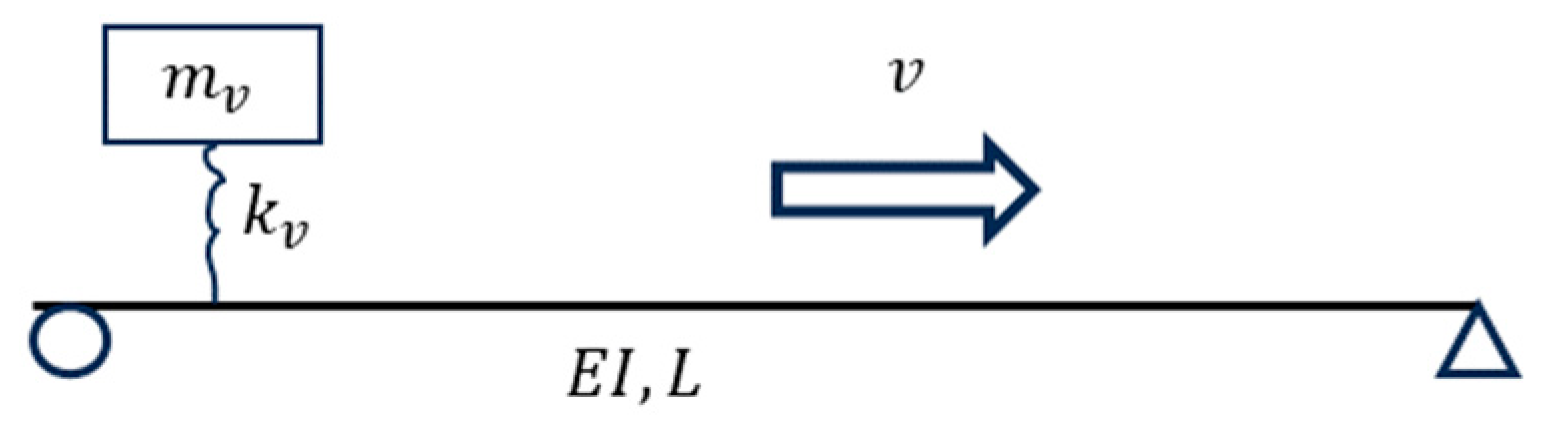
2.1. Dynamics of a Typical VBI System

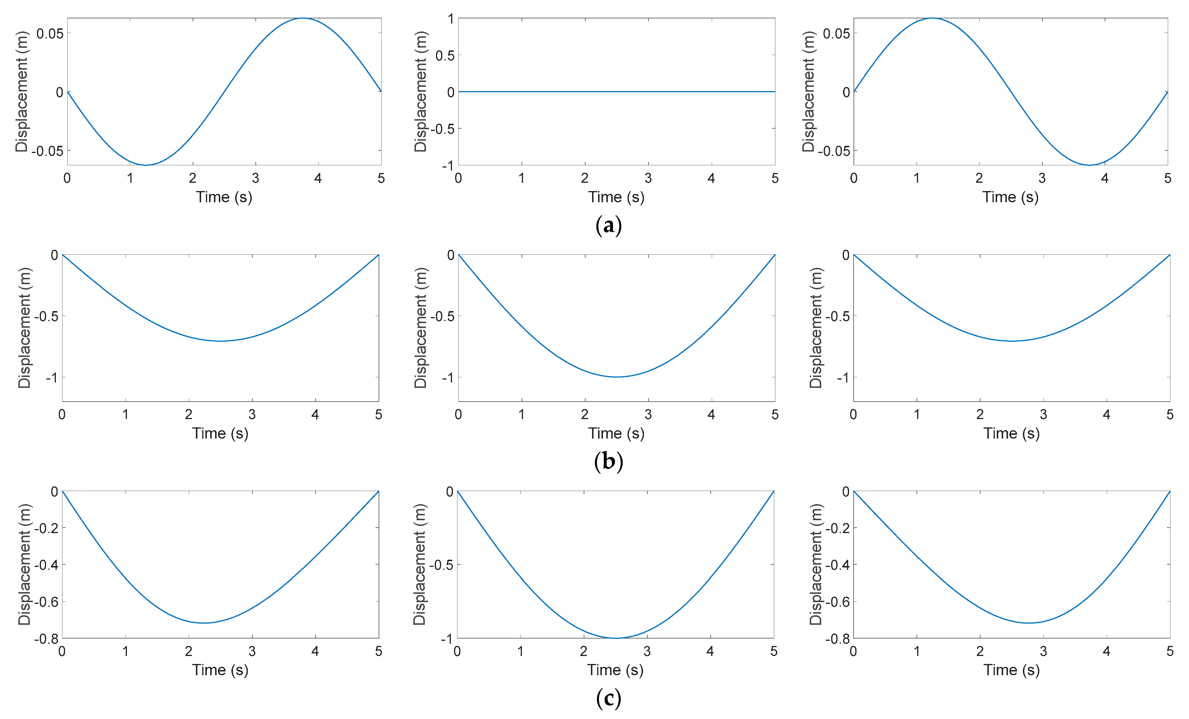
2.1.1. Dynamic Equations and Modal Responses

A schematic representation of a typical simple vehicle–bridge interaction (VBI) system is depicted in Figure 1, comprising a simply supported beam and a moving sprung mass traverses at a uniform velocity, v. The dynamic equations governing the system’s behavior are articulated as follows [30]:

For the vehicle,

$$\begin{array}{c}{m}_v{\ddot{q}}_v+k_v{q}_v=k_v {\left.u\right|}_{x=vt}\end{array}$$

(1)

For the bridge,

$$\begin{array}{c}\overline{m}\ddot{u}+EI{u}^{\prime \prime \prime \prime }=p\left(x,t\right)\end{array}$$

(2)

Elaborations of the symbols and abbreviations of all these equations are listed in the Appendix A. Road roughness was excluded from the analysis due to its minimal impact on bridge dynamics [37]. As Yang posited [30], in scenarios where the vehicle’s mass is significantly lower compared to the bridge’s mass, the force exerted via the vehicle, denoted as p(x,t), can be approximated as the moving vehicle’s gravitational force. Consequently, the dynamic responses of the bridge can be resolved as indicated [30]:

$$\begin{array}{c}u\left(x,t\right)={\displaystyle \sum _n}{\displaystyle \frac{{\Delta }_{stn}}{1-S_n^2}}\left\{sin{\displaystyle \frac{n\pi x}{L}}\right[\sin {\displaystyle \frac{n\pi vt}{L}}-S_n\sin {\omega }_{bn}t\left]\right\}\end{array}$$

(3)

where [30]

$${\Delta }_{st,n}={\displaystyle \frac{-2m_{v}g{L}^3}{n^4{\pi }^{4}EI}}$$

(4)

$$S_n={\displaystyle \frac{n\pi v}{L{\mathsf{\omega }}_{b,n}}}$$

(5)

$${\mathsf{\omega }}_{b,n}={\displaystyle \frac{n^2{\pi }^2}{L^2}}\sqrt{{\displaystyle \frac{EI}{\overline{m}}}}$$

(6)

The $u\left(x,t\right)$ in Equation (3) can be divided into two parts: the low-frequency part, $u_{low}\left(x,t\right)$, and the high-frequency part, $u_{high}\left(x,t\right)$ (shown in Equations (7) and (8)) [30].

$$u_{low}\left(x,t\right)={\sum }_n{\displaystyle \frac{{\Delta }_{stn}}{1-S_n^2}}\left[sin{\displaystyle \frac{n\pi x}{L}}\sin {\displaystyle \frac{n\pi vt}{L}}\right]$$

(7)

$$u_{high}\left(x,t\right)=\sum _n{\displaystyle \frac{{\Delta }_{stn}}{1-S_n^2}}[-sin{\displaystyle \frac{n\pi x}{L}}{S}_n\sin {\omega }_{bn}t]$$

(8)

It is important to highlight that the scope of this study, including the finite element simulations and field tests presented in subsequent sections, was primarily concentrated on long and slender beams, which are more representative of those commonly found in typical bridges. Consequently, in this theoretical segment, our analysis is confined to the Euler–Bernoulli beam model. Timoshenko beams, whose shear deformation plays a considerably significant role, are beyond the purview of this investigation.

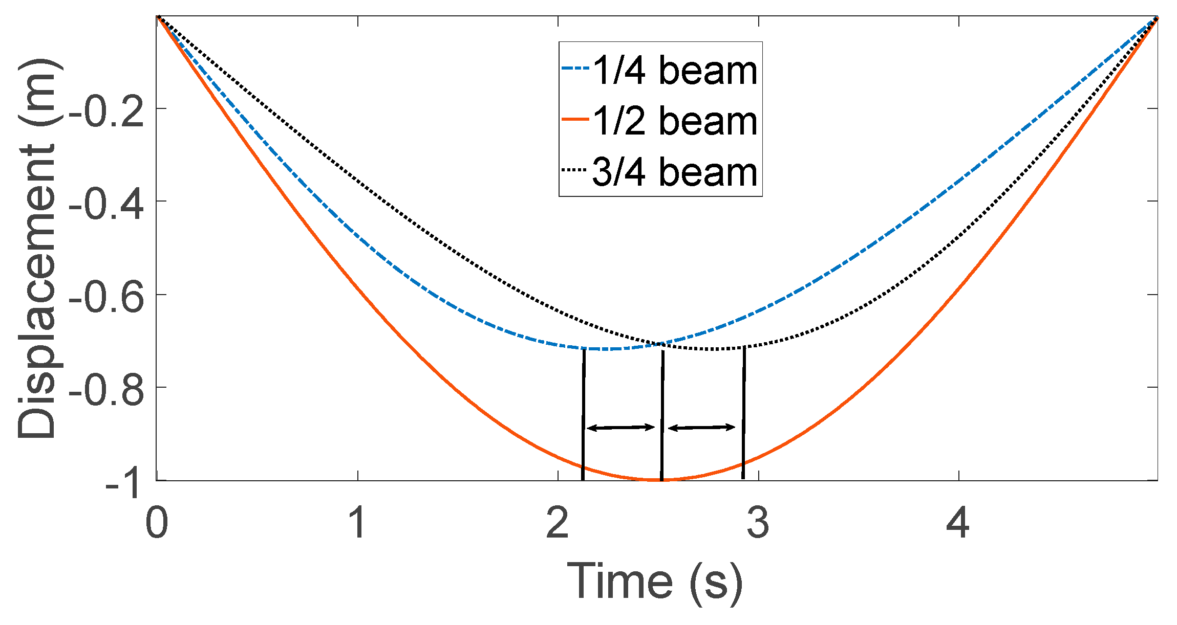
2.1.2. Time Lag in Low-Frequency Bridge Displacement

The concept of a time lag is traditionally perceived as a time-dependent phenomenon in the context of quasi-static bridge responses to vehicular loading. However, in this study, we delved into the examination of quasi-static bridge responses through the lens of low-frequency dynamic behavior.

As demonstrated by Fryba in [32], the low-frequency dynamic response $u_{low}\left(x,t\right)$ corresponds to the static deflection of the bridge, as depicted in Equation (9) [32], when subjected to a constant moving force, $m_{v}g$, when $S_n$ approaches zero.

$$\begin{gathered} u_{low}\left(x,t\right)=u_{static}\left(x,a\right) \\ =\left\{\begin{array}{c}{\displaystyle \frac{-m_{v}gx\left(L-a\right)}{6EIL}}\left(L^2-x^2-{\left(L-a\right)}^2\right) \left(a>x\right)\\ {\displaystyle \frac{-m_{v}g\left(L-a\right)}{6EIL}}\left({\displaystyle \frac{L}{L-a}}{\left(x-a\right)}^3+x\left(L^2-{\left(L-a\right)}^2\right)-x^3\right) \left(a<x\right)\end{array}\right. \end{gathered}$$

(9)

where

$$a=vt$$

(10)

As noted by Paultre et al. [38], $S_n$ approaches zero for typical highway bridges. Consequently, Equation (9) can be regarded as approximately valid under such conditions. It is important to recognize that the calculation of $u_{static}\left(x,a\right)$ is based on a static mechanical perspective, which assumes the absence of bridge damping. Accordingly, in this study, the computation of $u_{low}\left(x,t\right)$ intentionally disregarded the potential impacts arising from damping effects.

The “time-lag” phenomenon can be inferred from the right-hand side of Equation (9), where the temporal instances corresponding to the maximum bridge deflection vary for sensors situated at distinct locations. While the function $u_{static}\left(x,a\right)$ is piecewise, with its inflection point and the moment of peak deflection being time-dependent, Equation (7) illustrates that $u_{low}\left(x,t\right)$ is a superposition of sinusoidal time functions, specifically $\sin {\displaystyle \frac{n\pi vt}{L}}$. It is crucial to observe that these sinusoidal functions in the time domain are uniform across different locations, such as $x_1$ and $x_2$. The disparity in the responses at $x_1$ and $x_2$ should be attributable to the modal coordinates, that is, $sin{\displaystyle \frac{n\pi x}{L}}$. Hence, the time lag can be elucidated with the divergence in modal coordinates.

For instance, as depicted in Figure 2a, the low-frequency vertical displacement of the bridge at the 1/4, 1/2, and 3/4 points of the beam length is presented for the first mode (n = 1 in Equation (7)). Figure 2b displays the low-frequency bridge displacement in the second mode at the same three locations. Figure 2c demonstrates the combined effect of the displacements from the first and second modes. Moreover, Equation (7) indicates that higher modes contribute minimally to the displacement, $u_{low}\left(x,t\right)$. The displacement amplitude ratio for each low-frequency mode follows a pattern of (1, 1/2⁴, 1/3⁴, … 1/n⁴). Figure 2c reveals that the aggregate displacement is approximately equivalent to $u_{low}\left(x,t\right)$. Figure 3 provides a comparative analysis of the cumulative displacement. The time-lag phenomenon can thus be confirmed as an aggregate of multiple low-frequency modal vibrations.

2.1.3. Intersectional Relationship for the Simple VBI System

Specifically, the intersectional relationship for the aforementioned simple VBI system was derived. Sensors positioned at three distinct cross-sections, denoted as $x_1$, $x_2$, and $x_3$ were selected. The low-frequency bridge displacements at the N+1 time points were assumed to be the sequences {$u_{x_1,t_0}, u_{x_1,t_1, }\dots u_{x_1,t_N}$}, {$u_{x_2,t_0}, u_{x_2,t_1, }\dots u_{x_2,t_N}$}, and {$u_{x_3,t_0}, u_{x_3,t_1, }\dots u_{x_3,t_N}$}. In the case of medium-span and short-span bridges, the first two modes typically represent the global modes of the entire bridge and are the most significant contributors to the bridge’s dynamic responses. Consequently, the subsequent matrix equations (Equations (11) and (12)) can be deduced from Equation (7).

$$\left[\begin{array}{cc}sin{\displaystyle \frac{\pi x_1}{L}}& sin{\displaystyle \frac{2\pi x_1}{L}}\\ sin{\displaystyle \frac{\pi x_2}{L}}& sin{\displaystyle \frac{2\pi x_2}{L}}\end{array}\right]\left[\begin{array}{cccc}{\displaystyle \frac{{\Delta }_{st,1}}{1-S_1^2}}sin{\displaystyle \frac{\pi v{t}_0}{L}}& {\displaystyle \frac{{\Delta }_{st,1}}{1-S_1^2}}sin{\displaystyle \frac{\pi v{t}_1}{L}}& \cdots & {\displaystyle \frac{{\Delta }_{st,1}}{1-S_1^2}}sin{\displaystyle \frac{\pi v{t}_N}{L}}\\ {\displaystyle \frac{{\Delta }_{st,2}}{1-S_2^2}}sin{\displaystyle \frac{2\pi v{t}_0}{L}}& {\displaystyle \frac{{\Delta }_{st,2}}{1-S_2^2}}sin{\displaystyle \frac{2\pi v{t}_1}{L}}& \cdots & {\displaystyle \frac{{\Delta }_{st,2}}{1-S_2^2}}sin{\displaystyle \frac{2\pi v{t}_N}{L}}\end{array}\right]=\left[\begin{array}{cccc}{u}_{x_1,t_0}& u_{x_1,t_1}& \cdots & u_{x_1,t_N}\\ u_{x_2,t_0}& u_{x_2,t_1}& \cdots & u_{x_2,t_N}\end{array}\right]$$

(11)

$$\left[\begin{array}{cc}sin{\displaystyle \frac{\pi x_2}{L}}& sin{\displaystyle \frac{2\pi x_2}{L}}\\ sin{\displaystyle \frac{\pi x_3}{L}}& sin{\displaystyle \frac{2\pi x_3}{L}}\end{array}\right]\left[\begin{array}{cccc}{\displaystyle \frac{{\Delta }_{st,1}}{1-S_1^2}}sin{\displaystyle \frac{\pi v{t}_0}{L}}& {\displaystyle \frac{{\Delta }_{st,1}}{1-S_1^2}}sin{\displaystyle \frac{\pi v{t}_1}{L}}& \cdots & {\displaystyle \frac{{\Delta }_{st,1}}{1-S_1^2}}sin{\displaystyle \frac{\pi v{t}_N}{L}}\\ {\displaystyle \frac{{\Delta }_{st,2}}{1-S_2^2}}sin{\displaystyle \frac{2\pi v{t}_0}{L}}& {\displaystyle \frac{{\Delta }_{st,2}}{1-S_2^2}}sin{\displaystyle \frac{2\pi v{t}_1}{L}}& \cdots & {\displaystyle \frac{{\Delta }_{st,2}}{1-S_2^2}}sin{\displaystyle \frac{2\pi v{t}_N}{L}}\end{array}\right]=\left[\begin{array}{cccc}{u}_{x_2,t_0}& u_{x_2,t_1}& \cdots & u_{x_2,t_N}\\ u_{x_3,t_0}& u_{x_3,t_1}& \cdots & u_{x_3,t_N}\end{array}\right]$$

(12)

The responses at $x_3$ can then be calculated from Equation (13).

$$\left[\begin{array}{cccc}{u}_{x_2,t_0}& u_{x_2,t_1}& \cdots & u_{x_2,t_N}\\ u_{x_3,t_0}& u_{x_3,t_1}& \cdots & u_{x_3,t_N}\end{array}\right]=\left[\begin{array}{cc}sin{\displaystyle \frac{\pi x_2}{L}}& sin{\displaystyle \frac{2\pi x_2}{L}}\\ sin{\displaystyle \frac{\pi x_3}{L}}& sin{\displaystyle \frac{2\pi x_3}{L}}\end{array}\right]{\left[\begin{array}{cc}sin{\displaystyle \frac{\pi x_1}{L}}& sin{\displaystyle \frac{2\pi x_1}{L}}\\ sin{\displaystyle \frac{\pi x_2}{L}}& sin{\displaystyle \frac{2\pi x_2}{L}}\end{array}\right]}^{-1}\left[\begin{array}{cccc}{u}_{x_1,t_0}& u_{x_1,t_1}& \cdots & u_{x_1,t_N}\\ u_{x_2,t_0}& u_{x_2,t_1}& \cdots & u_{x_2,t_N}\end{array}\right]$$

(13)

The transform matrix is then defined as $T$. For this simple VBI system,

$$T=\left[\begin{array}{cc}sin{\displaystyle \frac{\pi x_2}{L}}& sin{\displaystyle \frac{2\pi x_2}{L}}\\ sin{\displaystyle \frac{\pi x_3}{L}}& sin{\displaystyle \frac{2\pi x_3}{L}}\end{array}\right]{\left[\begin{array}{cc}sin{\displaystyle \frac{\pi x_1}{L}}& sin{\displaystyle \frac{2\pi x_1}{L}}\\ sin{\displaystyle \frac{\pi x_2}{L}}& sin{\displaystyle \frac{2\pi x_2}{L}}\end{array}\right]}^{-1}$$

(14)

The matrix $T$ represents the target intersectional relationship, which is utilized to derive the displacement $\{ u_{x_3,t_N}\}$ from the measured $\{ u_{x_1,t_N}$} and {$u_{x_2,t_N}$}. This matrix, T, is solely dependent on the bridge’s mode shapes, and it is invariant with time. Furthermore, T is independent of traffic conditions, which are characterized by the term {${\displaystyle \frac{{\Delta }_{st,n}}{1-S_n^2}}$}. Additionally, while fluctuations in air temperatures may influence the global material stiffness of the bridge, T retains its time-invariant property as long as the mode shapes remain unchanged. In the context of the estimation process, it is advisable to employ monitoring data from a minimum of two cross-sections. This ensures that the information obtained encompasses at least the first two principal modes of the bridge’s dynamic behavior.

2.1.4. From a Simple Model to a General Bridge Structure

In typical bridge structures, the solution derived from Equation (3) can be generalized as a product of the modal shapes and their corresponding modal coordinates, as articulated in Equation (15).

$$u\left(x,t\right)={\sum }_n{\varnothing }_n\left(x\right)q_{b,n}\left(t\right)$$

(15)

For example, we chose two arbitrary observation points, $x_1$ and $x_2$. In accordance with Equation (15), the vertical displacements at $x_1$ and $x_2$ should be

$$u\left(x_1,t\right)=\sum _n{\varnothing }_n\left(x_1\right)q_{b,n}\left(t\right)$$

(16)

$$u\left(x_2,t\right)=\sum _n{\varnothing }_n\left(x_2\right)q_{b,n}\left(t\right)$$

(17)

Equations (16) and (17) can be reformatted into matrix form, as presented in Equations (18) and (19).

$$u\left(x_1,t\right)={\varnothing }_n\left(x_1\right)q_{b,n}\left(t\right)$$

(18)

$$u\left(x_2,t\right)={\varnothing }_n\left(x_2\right)q_{b,n}\left(t\right)$$

(19)

where are corresponding matrices or vectors. The intersection relationship is represented as $T$, which transforms $u\left(x_1,t\right)$ into $u\left(x_2,t\right)$ (as shown in Equation (20)).

$$u\left(x_2,t\right)=Tu\left(x_1,t\right)$$

(20)

Substituting Equations (18) and (19) into Equation (20), one can confirm that

$$T={\left\{{\varnothing }_n\left(x_1\right)\right\}}^{+}{\varnothing }_n\left(x_2\right)$$

(21)

where the $+$ denotes the generalized inverse. Equation (21) illustrates that the matrix $T$ is independent of time and is solely associated with the mode shapes. Furthermore, Equations (18) and (19) indicate that the dynamic responses $x_1$ and $x_2$ should share the same time-domain coordinate, $q_{b,n}(t)$. Although $q_{b,n}(t)$ may change under varying traffic conditions, vehicle characteristics, and moving speeds, this time-domain coordinate remains consistent across different cross-sections. Consequently, $T$ should be exempt from the influence of time-varying traffic conditions. Additionally, it is postulated that the time-independent nature of the intersectional relationship should also extend to complex bridge structures, provided that the dynamic responses can be articulated through Equation (21) in conjunction with the time-independent mode shape function, ${\varnothing }_n\left(x\right)$.

It is important to note that Equation (21) also highlights the distinction between the current study and existing research. In prior studies, low-frequency bridge responses, referred to as “quasi-static responses,” were analyzed from a static perspective. These quasi-static responses are influenced by time-varying factors, including external loading, which is dictated by traffic conditions, and material stiffness, which can be affected by air temperatures. Moreover, as suggested in the right side of Equation (9), the transfer function between responses at different cross-sections appears to be time-dependent. However, in this study, we adopted a dynamic analysis approach to treat low-frequency responses. As demonstrated in Equations (14) and (21), the transfer matrix should remain time-invariant, regardless of changes in traffic conditions and air temperatures. This fundamental difference also informed our choice of the subsequent response-estimation method.

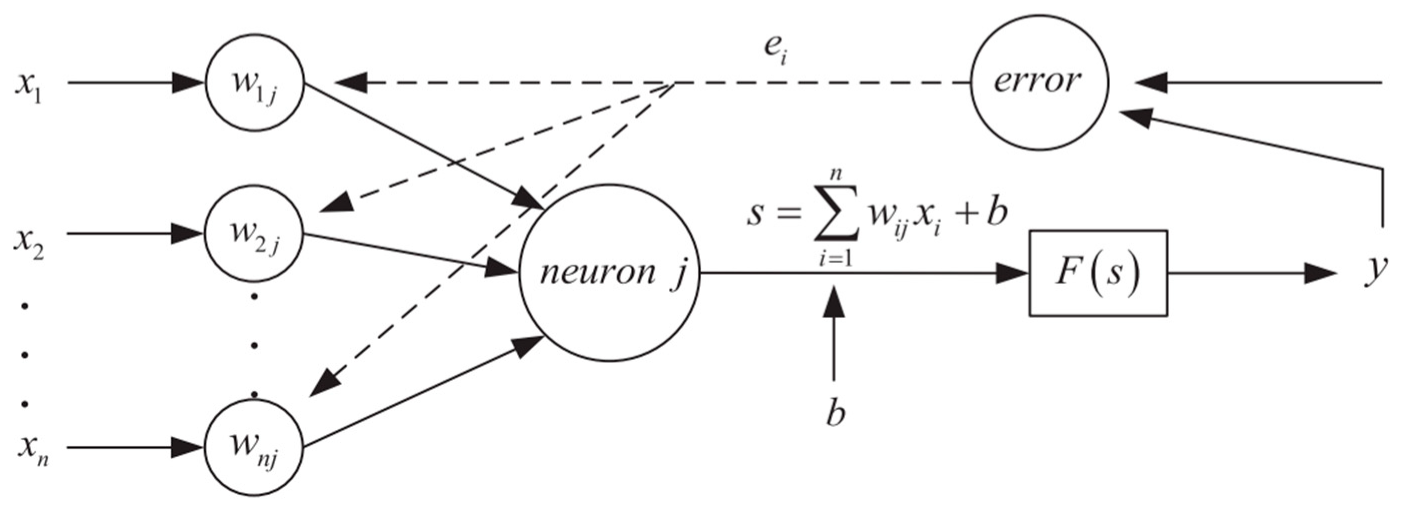
2.2. BP-ANN for Intersection Responses Prediction

The hypothesis was that the intersectional relationship, as per Equation (21), should remain time-independent under fluctuating temperatures and vehicle loading conditions. Consequently, diverging from the time-series prediction methods employed in previous studies, it was assumed that there was no necessity to account for time-related factors in the response estimation process. To simulate the target relationship and subsequently estimate the responses at a specific cross-section, a BP-ANN was utilized for training. It is crucial to emphasize that the BP-ANN network was designed with a time-invariant structure, aligning with the time-independent relationship established in Equation (21). Furthermore, the adoption of BP-ANN was expected to eliminate the need to train any superfluous time-related factors, which are typically associated with time-series prediction methods in existing research. This approach was anticipated to be more time-efficient compared to traditional time-series prediction techniques.

In the process of training the network, responses from several cross-sections were configured as multiple inputs, whereas the responses at a particular section served as the output. A mapping relationship was subsequently trained to emulate the intersectional relationship. This trained network, informed by Equation (21), should be able to capture long-term intersectional dynamics under varying traffic conditions and air temperatures, effectively utilizable even without traffic condition or air temperature information.

A typical backpropagation neural network structure [33] consists of artificial neuron units, as shown in Figure 4, where $x_i(i=\mathrm{1,2},\dots n)$ denotes the input of the current unit, j. $w_{ij}$ is the weight corresponding to each input. Then, the output, y, of the unit, j, can be calculated as follows:

$$s=\sum _{i=1}^n{w}_{ij}{x}_i+b$$

(22)

$$y=F\left(s\right)={\displaystyle \frac{1}{1+e^{-s}}}$$

(23)

in which b is the bias term.

Backpropagation neural networks are composed of input layers, output layers, and hidden layers, as depicted in Figure 5. Each layer is made up of one or more artificial neuron units. During model training, these units take in the output from the preceding layer and process it to produce the input for the subsequent layer. The weights and biases are adjusted through an iterative process aimed at minimizing the overall error, in accordance with Equations (24) and (25) [33].

$$w\left(k+1\right)=w\left(k\right)-\mathsf{\alpha }{\displaystyle \frac{\partial E\left(k\right)}{\partial w\left(k\right)}}$$

(24)

$$b\left(k+1\right)=b\left(k\right)-\mathsf{\alpha }{\displaystyle \frac{\partial E\left(k\right)}{\partial b\left(k\right)}}$$

(25)

in which,

$$E\left(k\right)=\sqrt{{\displaystyle \frac{1}{N}}\sum _{i=1}^N{\left|e_i\right|}^2}$$

(26)

The network architecture is depicted in Figure 5. For instance, let us consider a scenario where responses at m + 1 cross-sections are measured. The time-series responses at the first m cross-sections are then employed as m inputs, while the responses at the m + 1 cross-section are designated as the output. Specifically, for each set of inputs and outputs, each neuron contains a single time-point value. Under the guidance of Equation (21), the network does not incorporate time-dependent information regarding traffic conditions and temperature. Moreover, the mode shapes represented in all of these inputs should include the mode shape component present in the output. If there exists a unique mode in the output that is orthogonal to all the modes in the input, it is anticipated that the model may not yield satisfactory results.

The network configuration is detailed as follows. The network comprises two hidden layers: the first layer consists of 128 neurons, and the second layer contains 32 neurons. The output layer is designed with a single neuron, which corresponds to the monitoring data at sensor 02-S01. The learning rate is configured at 0.001, the batch size is set to 100, and the number of epochs is 500. The activation function employed is the rectified linear unit (ReLU) function. During the training phase of the BP-ANN network, the sequential order of the time-series data is not taken into account. Data batches are formed randomly and used for training, which deviates from the conventional time-series prediction methods. This random batching approach ensures that no time-dependent characteristics are considered for the intersectional relationship. In the subsequent validation processes, as specifically outlined in Section 3.4 and Section 4.3.2, the network with this straightforward structure demonstrates its capability of providing accurate estimations for both finite element simulation and field-test data.

3. Numerical Analysis

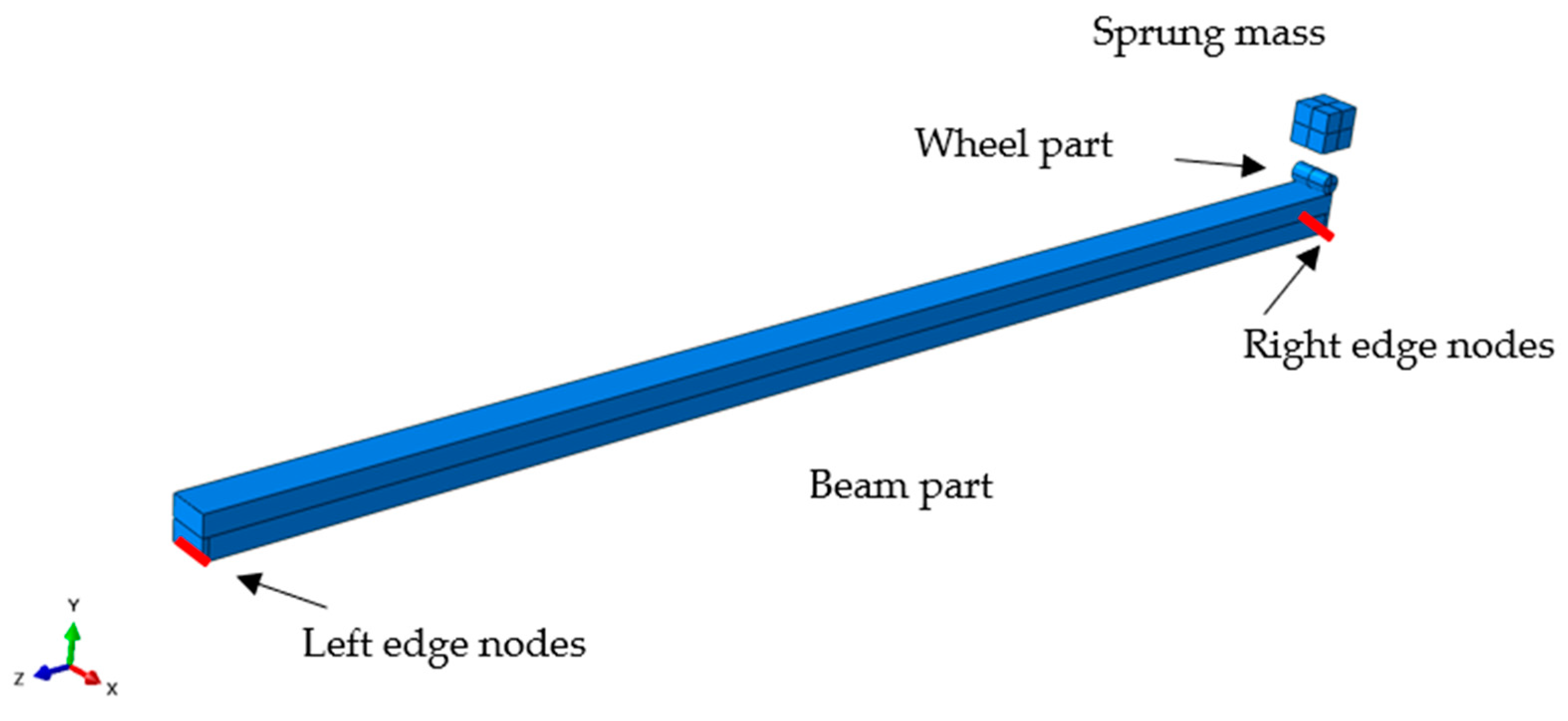
3.1. Numerical Models

In this study, a typical VBI system model [30] employed in a previous study was used. This model consists of a simply supported beam and a sprung mass as the moving vehicle. The beam span is L = 25 m. The unit beam mass per meter is $\overline{m}$ = 4800 kg/m. EI = 3.33 × 10⁹ N/m². The first three bending frequencies of the beam are 2.08 Hz, 8.33 Hz, and 18.75 Hz, respectively. The sprung mass is $m_v$ = 1200 kg, and the spring stiffness is $k_v$ = 500,000 N/m. The vibration frequency of the vehicle is 3.25 Hz.

The commercial software ABAQUS 2020 [39] was employed to construct a finite element model, as depicted in Figure 6, in order to simulate the VBI system. The model utilized three-dimensional solid elements to represent the beam, sprung mass, and wheel components. The element types, quantities, and mesh sizes for these components are detailed in

Table 1. Element properties of the finite element model.

Component	Type	Amount	Size (m × m × m)
Beam	C3D8R	16,128	0.1 × 0.1 × 0.1
Wheel	C3D8R	320	0.08 × 0.08 × 0.08
Sprung mass	C3D8R	8000	0.04 × 0.04 × 0.04

as follows:

The element size for the beam was set to 0.1 m × 0.1 m × 0.1 m, a decision informed by a mesh convergence study. As illustrated in Figure 7, the mid-span displacement exhibits minimal variation when the mesh size is finer than 0.15 m × 0.15 m × 0.15 m. The boundary conditions for the simply supported beam were established by restricting the appropriate degrees of freedom at the beam’s edge nodes, as indicated in Figure 6. For the left edge nodes, translations along the X, Y, and Z axes, as well as rotations about the Y and Z axes, were fixed. Similarly, translations along the X and Y axes and rotations around the Y and Z axes were restricted for the right edge nodes. Interaction was modeled with penalty method, and the interaction force was implicitly calculated and applied to the beam surface in contact with the wheel. Additionally, a spring element was employed to represent the spring constant between the sprung mass and the wheel. Road roughness was excluded from this model due to its minimal impact on low-frequency beam responses. The model responses were obtained using the Hilber–Hughes–Taylor α-method in the implicit calculation mode, which involves two main stages. The first stage involves applying gravity to the entire system, known as the “Static, Implicit” step, during which the vehicle is positioned at one end of the beam. The second stage is the “Dynamic, Implicit” step, during which time integration is performed with a time step of 0.01 s to compute the dynamic responses of the system. In this stage, the vehicle is moved from the initial position to the opposite end at a constant velocity [40].

3.2. Cases’ Configuration

This study was designed to validate the consistent intersectional relationship between low-frequency responses at different locations along the beam. In prior research focusing on “quasi-static” responses [12,13], the adoption of time-related time-series prediction methods is conventional, given that “quasi-static” responses, as depicted in Equation (9), are influenced by time-dependent traffic conditions. Furthermore, in practical engineering, the three principal factors of traffic conditions are vehicle weight, vehicle speed, and vehicle volume. However, in this study, we shifted our focus from “quasi-static” responses to the transfer matrix of low-frequency responses, which demonstrated independence from fluctuating traffic conditions. Therefore, it is essential to confirm the time-irrelevant, time-independent physical characteristic of the transfer matrix, as well as the efficacy of the proposed method. Consequently, four scenarios were devised to encompass variations in moving speed, vehicle weight, and vehicle volume, as shown in Figure 8:

(1)

Reference case, where the moving speed was set to 5 m/s;

(2)

High-speed case, where the moving speed was set to 10 m/s;

(3)

Half-mass vehicle case, where the sprung mass was half that of the reference case;

(4)

Dual-vehicle case: The half-mass vehicle and the reference vehicle were running on the beam simultaneously. The high-frequency vehicle was moving at a speed of 3 m/s, while the reference vehicle was moving at a speed of 5 m/s.

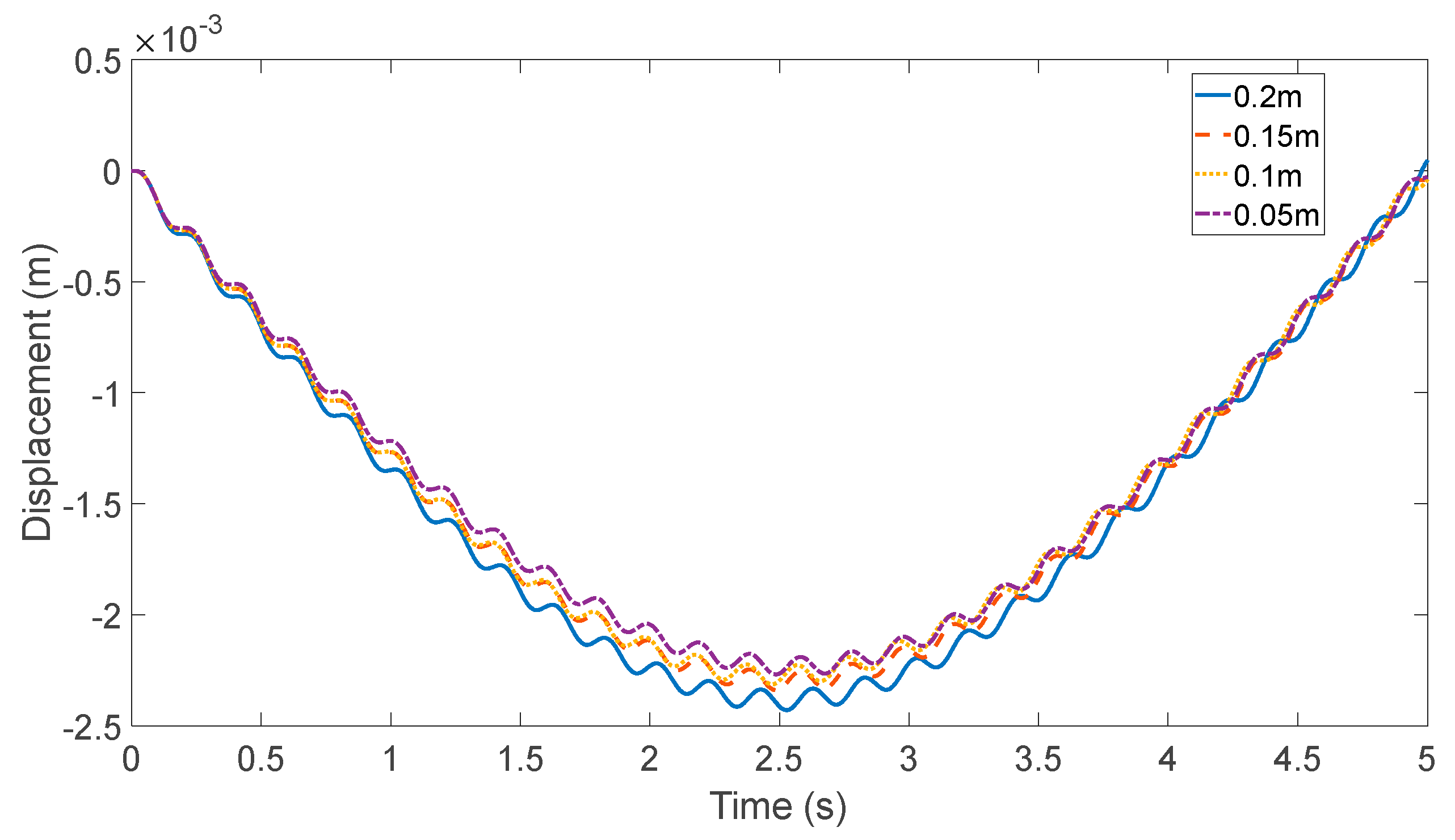
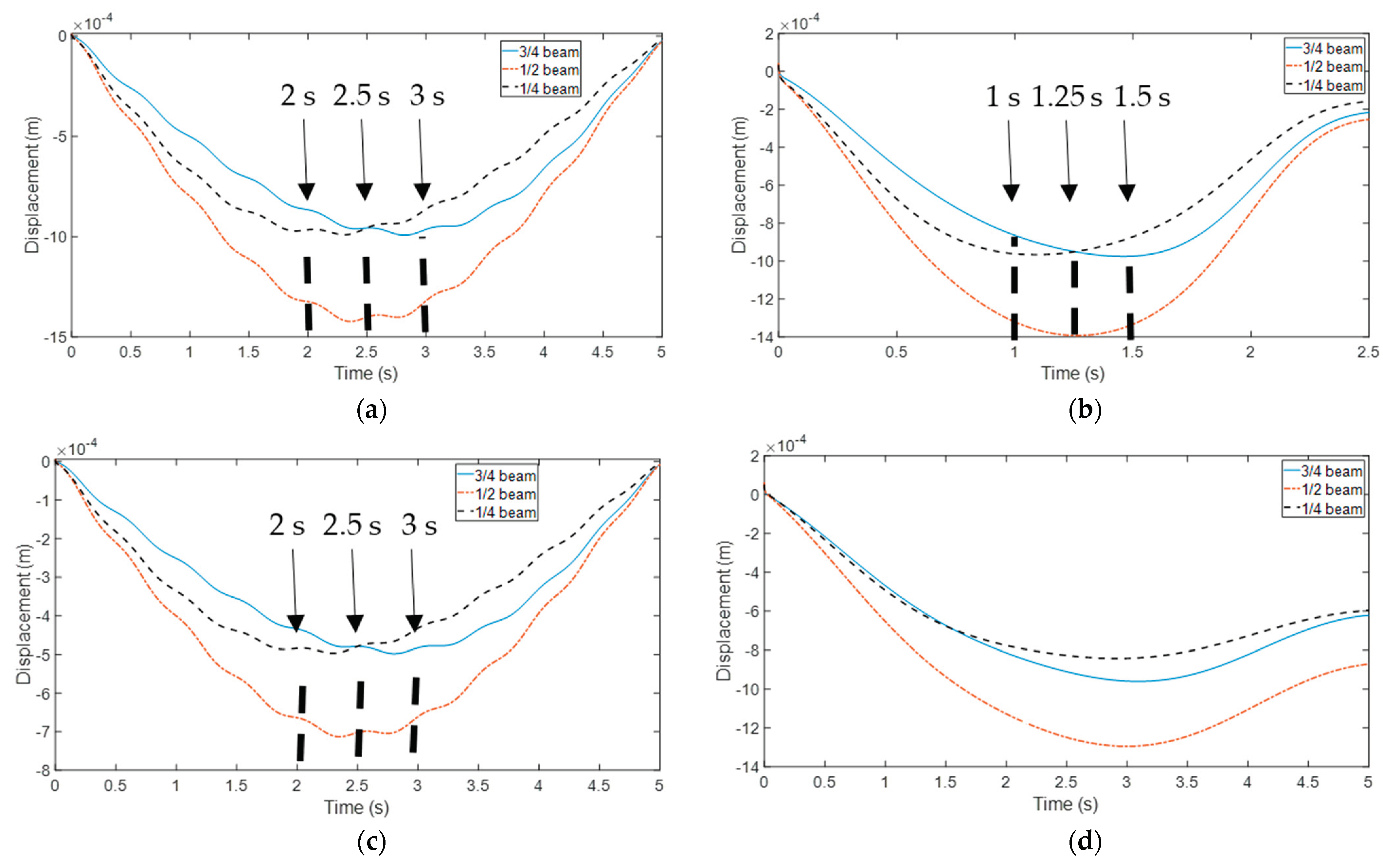
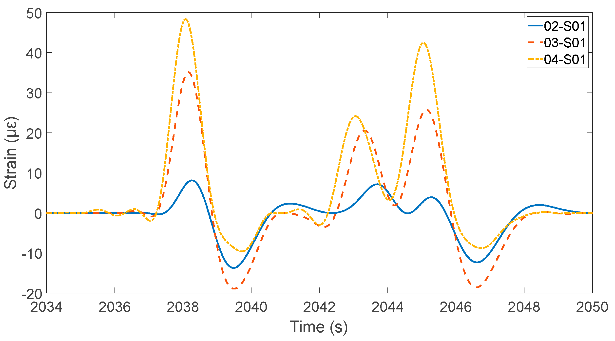
3.3. Simulation Result Analysis

The phenomenon of a “time lag” was initially investigated. Figure 9, panels (a) to (d), depict the time history of the vertical displacement of the beam at three cross-sections: the 3/4 point, the 1/2 point, and the 1/4 point of the beam’s length, across the four cases. It is apparent that the primary cause of the bridge’s displacement is the low-frequency responses associated with the driving force, a finding that aligns with Yang’s research [30]. Moreover, the time-lag phenomenon is quite pronounced. In Figure 9, the dashed lines highlight the time lag between the responses at different cross-sections, especially for the first three cases.

The consistently time-independent relationship between cross-sections was subsequently scrutinized. Specifically, the low-frequency vertical displacement time history at the 1/4 point of the beam was estimated using the data from the 1/2 and 3/4 points. The transfer matrix, derived from Equation (14), was employed to predict the low-frequency responses at the 1/4 point of the beam across all four cases. It is important to note that the same transfer matrix was applied to all scenarios. A cut-off frequency of 1 Hz was used to isolate the low-frequency displacement components. As evidenced in Figure 10, the estimated low-frequency vertical displacement at the 1/4 point of the beam closely aligns with the simulation outcomes in all four cases. Thus, it can be concluded that the intersectional relationship under scrutiny is indeed time-independent and remains constant across varying traffic conditions, including vehicle mass, speed, and passage time. Furthermore, since the transfer matrix is dictated by the bridge’s mode shape, and since alterations in global material stiffness do not modify the mode shape, changes in temperature, which might affect the bridge’s material stiffness, should not influence the intersectional relationship. Consequently, this section does not delve into potential numerical simulations associated with temperature variations.

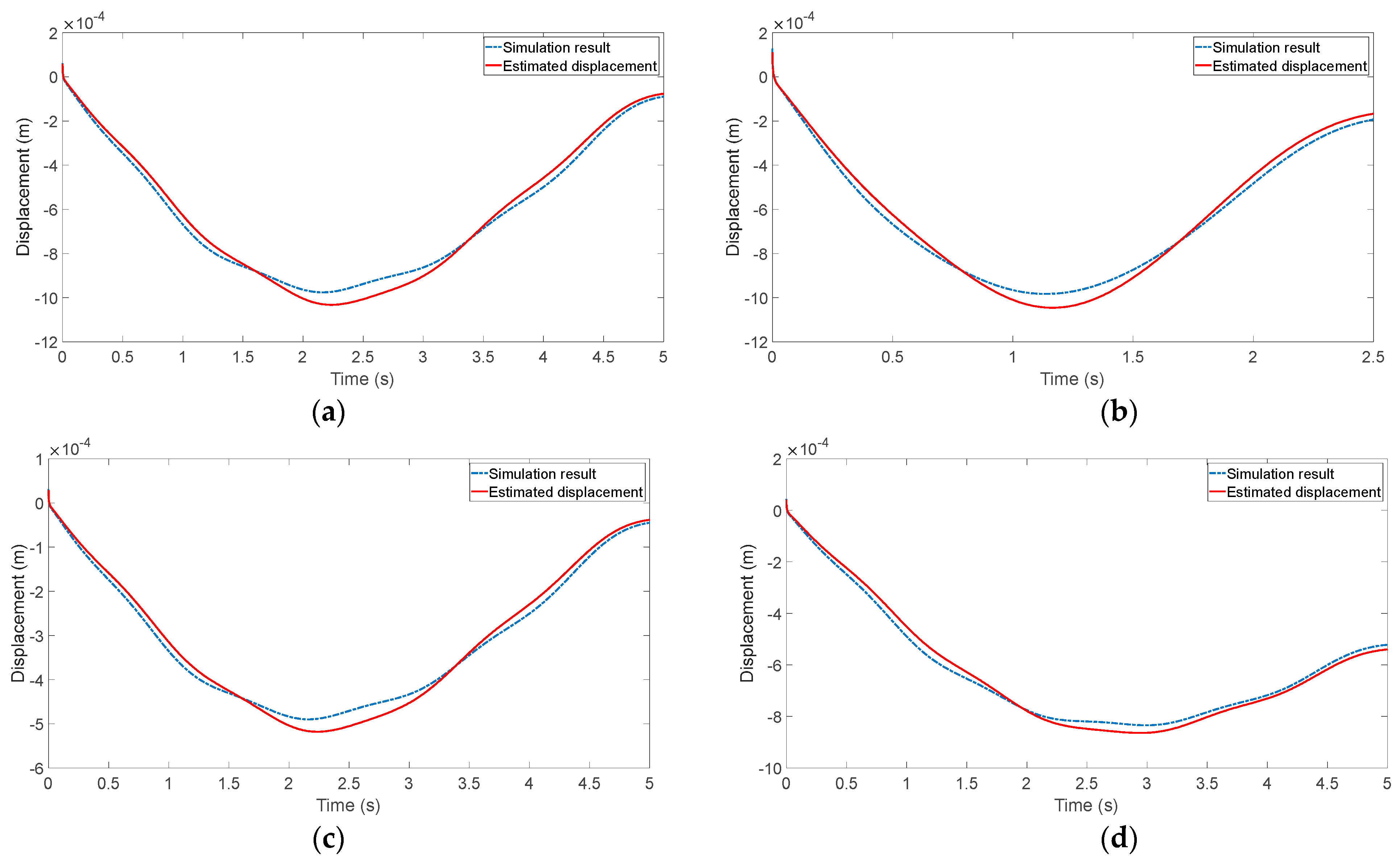
3.4. Validation of the BP-ANN with the Simulation Data

To substantiate the effectiveness of BP-ANN and assess its robustness, simulated data from the first three cases were used to train a BP-ANN model, while data from the fourth case were employed to evaluate the model’s performance. It is important to note that these simulations incorporated 5% white noise.

The network architecture includes an input layer with two neurons, corresponding to the displacements at the 1/2 and 3/4 points of the beam. Figure 11 presents a comparison between the noisy displacement of the simulation results and the displacement estimates derived from the BP-ANN. Both the peak values and the complete time history records show a close match. Thus, it can be concluded that the proposed method demonstrates robustness and performs effectively even in the presence of noise.

4. Validation with Field Test on a Continuous Bridge

In the preceding sections, we detailed the theoretical derivations and finite element simulations specifically for a simply supported bridge. However, in accordance with Equation (21), the proposed estimation method is not limited to this bridge type and can be extended to various other types of bridges. Furthermore, while our previous analysis focused solely on low-frequency displacement, the method we propose is also applicable to a broader range of bridge response indicators. In this section, we proceed to validate the proposed method using field test data measured on a real continuous bridge..

4.1. Target Bridge and SHM System

The target bridge is a concrete highway overpass situated in Hebei Province, China. It is a separate bridge structure on Baofu Highway, with distinct left and right sides. The left side comprises four continuous spans measuring 133 m (32 m + 32 m + 37 m + 32 m), and it is constructed with prestressed box girders, as depicted in Figure 12a [36]. The total length of the right side spans 179 m, consisting of a 75-m section (3 × 25 m) made up of prestressed concrete T-beams and a 104-m section (35 m + 37 m + 32 m) of a continuous prestressed box girder [41]. For more comprehensive geometric details of the bridge, reference [41] can be consulted.

In 2018, a structural health monitoring (SHM) system was installed to monitor responses of the target bridge, as illustrated in Figure 12b. The first two natural vibration frequencies of the bridge were previously determined using the stochastic subspace identification (SSI) method, measuring 3.906 Hz and 5.01 Hz, respectively [41]. The structural health monitoring (SHM) system is equipped with an array of sensors, including strain gauges, thermometers, accelerometers, and so on. For the purposes of this study, we utilized only the strain gauges mounted on Section 02, which is approximately at the 1/4 point of the fourth span, Section 03 (the midpoint section), and Section 04 (the 3/4 point of the fourth span). There are a total of twelve strain gauges installed across these three cross-sections (02, 03, and 04), with strain data being sampled at a frequency of 50 Hz. Further details regarding the SHM system can be found in the referenced study [42]. Although the previous section focused exclusively on bridge displacement and the intersectional relationship of displacement, it was anticipated that the strain time history would exhibit characteristics similar to those of the low-frequency bridge displacement. This expectation was grounded in the fact that the low-frequency bridge displacement under vehicular loading closely mimics the static displacement under a moving force. Moreover, in static scenarios, a relationship exists between the bending moment at a cross-section and the displacement at that section,

$$M\left(x\right)=-EI{\displaystyle \frac{d^{2}u}{d{x}^2}}$$

(27)

where $M\left(x\right)$ is the moment. Also, the moment is linearly proportional to the strain. Therefore, similar to Equation (3), the following function (Equation (28)) can be generated.

$$\epsilon \left(x,t\right)={\sum }_n{\varnothing }_{\epsilon ,n}\left(x\right)q_{\epsilon ,n}\left(t\right)$$

(28)

The strain mode shape function is represented by ${\varnothing }_{\epsilon ,n}\left(x\right)$, and the corresponding coefficient in the time domain is $q_{\epsilon ,n}\left(t\right)$. Additionally, the physical properties of the intersection displacement relationship, including the time-independent and constant properties, should also be available for the intersectional bridge strain under vehicular loading.

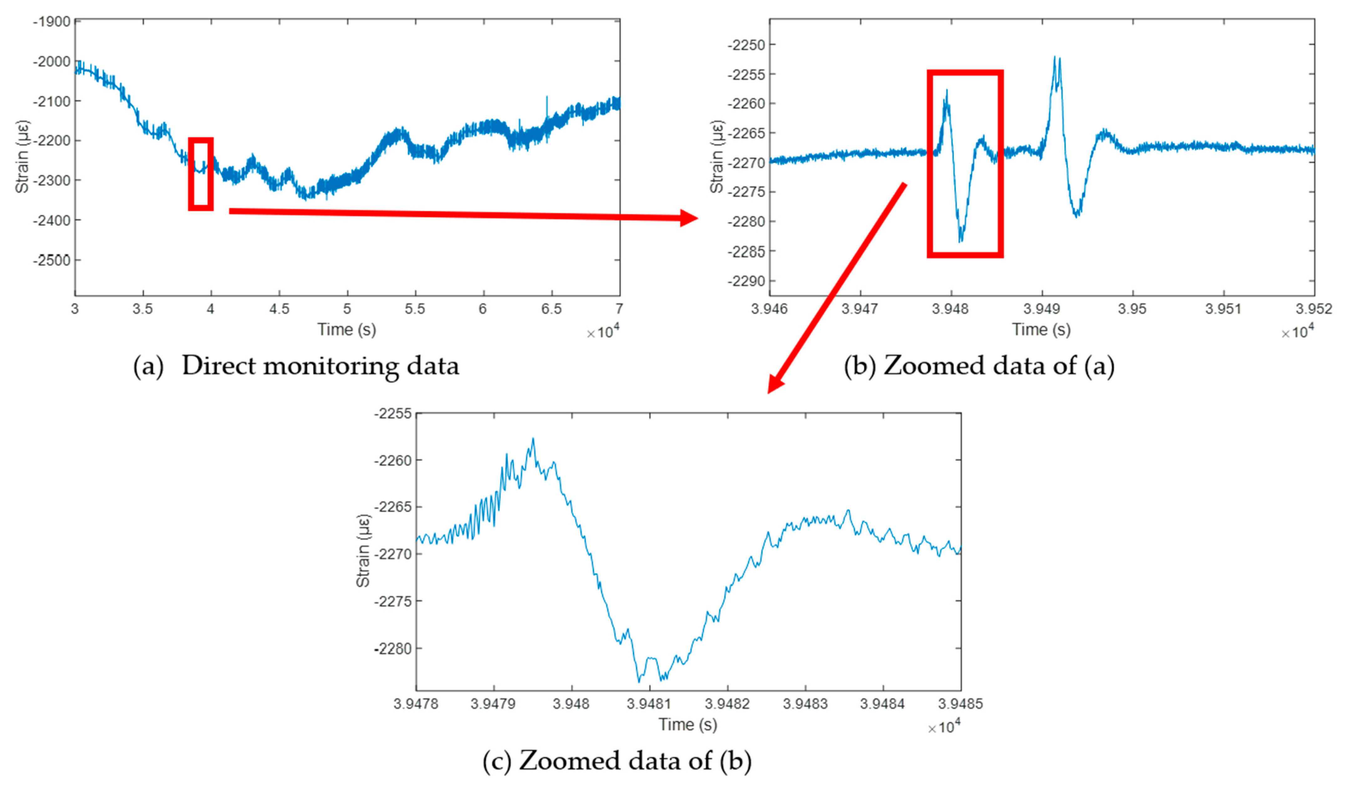
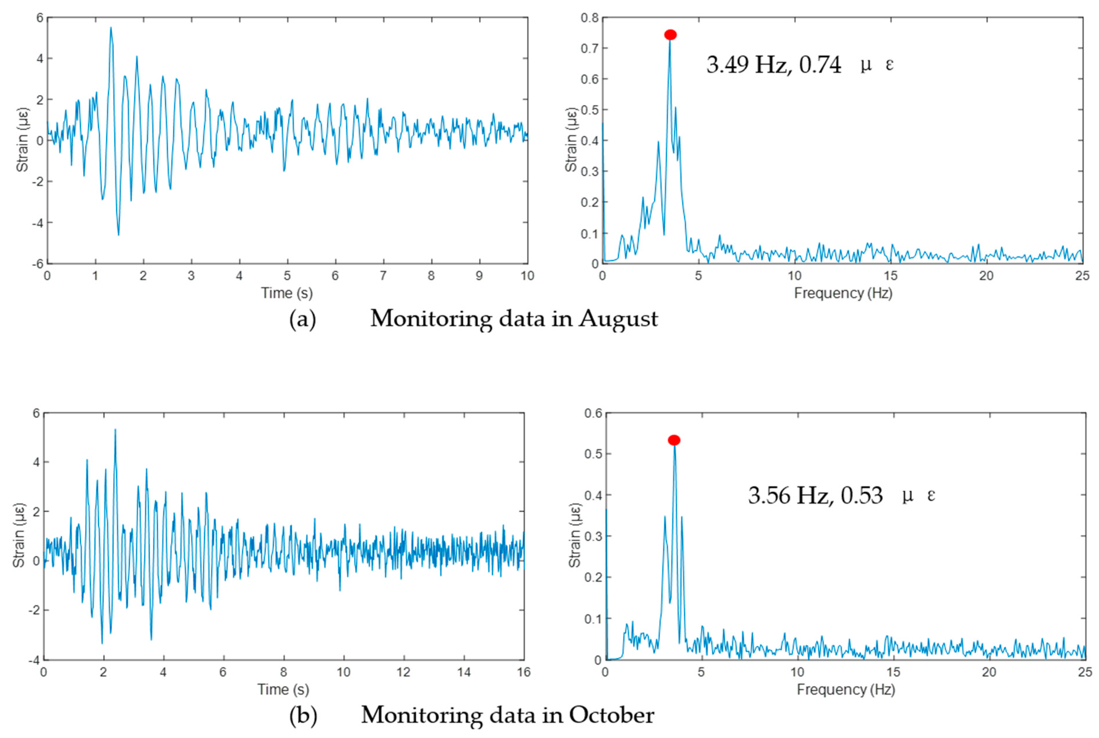
4.2. Monitoring Data

Figure 13 presents a typical piece of monitoring data. The strain variations depicted in Figure 13a are predominantly due to temperature fluctuations. Notably, there are several local “peaks” on the curve in Figure 13a, which are attributable to passing vehicles (with zoomed-in views provided in Figure 13b,c). It is evident that the strain induced via temperature changes exhibits a significantly higher amplitude compared to that caused by vehicle loading. Figure 13b illustrates that the amplitude of the low-frequency strain, induced via vehicle loading, is substantially greater than that of the high-frequency strain. This observation is further supported by Figure 13c, which shows numerous high-frequency, low-amplitude peaks in the strain time history. It is important to note that this study concentrated solely on low-frequency responses. As documented in prior research [37,38], the low frequencies associated with driving forces are considerably lower than the natural vibration frequencies of bridges. Moreover, the typical natural frequencies of short- and medium-span bridges exceed 1 Hz. To eliminate high-frequency strains, a low-pass filter [43] with a cutoff frequency of 1 Hz was employed in this study. The bridge’s natural vibration frequencies, while relevant, were not essential for the current investigation. The temperature-induced strain was estimated using a moving-mean method [43] and subsequently removed. This process yielded the low-frequency strain induced via vehicle loading. It should be mentioned that, in this study, the bridge strain was measured at only three cross-sections, which is insufficient for determining bridge-mode shapes using conventional methods such as SSI [3,4]. However, as outlined in the introduction, the proposed method addresses this limitation, as detailed below.

In this research, we utilized monitoring data from Section 03 and Section 04 to estimate the dynamic responses at Section 02. Specifically, data from sensors 03-S01 and 04-S01 were employed to forecast the data at 02-S01. Consequently, the input layer of the BP-ANN features two neuron units, each corresponding to the monitoring data from 03-S01 and 04-S01, respectively. When training the network, instead of inputting time-series data directly into the input layer’s neuron units, the BP-ANN processed discrete data points measured at specific time intervals. In more elaborate terms, with two input neuron units, each set of input data, comprising two values, was assigned to one neuron unit each. This approach marks a significant departure from the time-series prediction methods used in previous studies [17,18,19,20,21,22,23,24,25,26,27,28]. Although the estimation outcomes in this study are presented as time series of monitoring data, they are, in essence, a collection of discrete output values derived from the BP-ANN using discrete input data sets. A key advantage of this method is that it circumvents the need to calculate time-related factors, which are often required in traditional time-series prediction models.

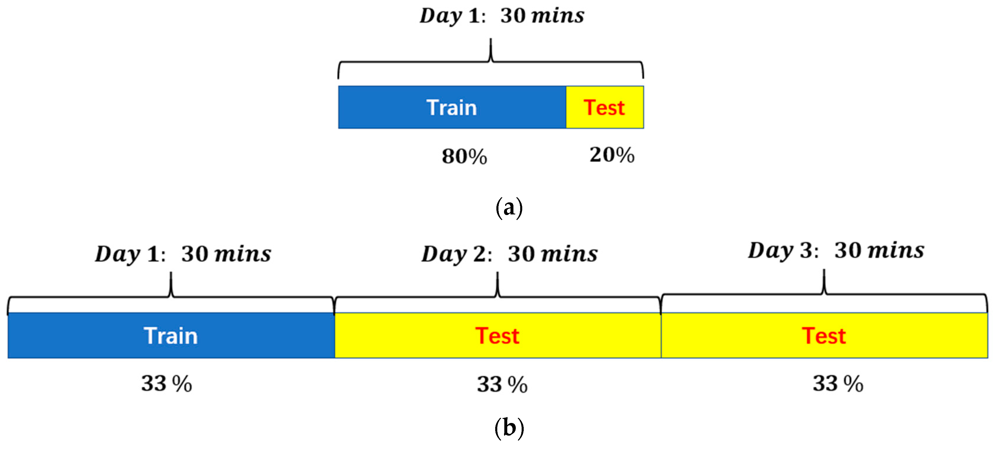
4.3. Scenarios and Data Configuration

4.3.1. Confirmation of Time Lag, Random Traffic Condition, and Temperature Effect

The time-lag phenomenon was evident in the time history of low-frequency strain induced via vehicle loading. Figure 14 illustrates the time history of low-frequency strain at these three cross-sections within a monitored segment. Similar to the observations in Figure 13b, a distinct peak, attributed to the passage of a vehicle, is visible in the strain time history. The time histories from the three gauges were superimposed, revealing discernible differences in the time instances at which peak amplitudes occurred. This observation confirms the presence of the time-lag phenomenon.

Traffic conditions were not specifically documented; however, the test data set encompassed scenarios featuring both single and multiple vehicles traversing the bridge, as depicted in Figure 14 and Figure 15, respectively. In Figure 15, the duration of the recorded vibration data significantly exceeds the typical transit time for a standard vehicle, suggesting that multiple vehicles were crossing the bridge during the monitoring interval. For these scenarios, details such as the number of vehicles, their mass, the frequency of passage, and the speed were unknown and anticipated to fluctuate. This variability ensures the broad applicability of the proposed method across a range of traffic conditions.

The monitoring data set also accounts for varying temperature conditions. For illustration, two segments of monitoring data were selected: one from 28 August (summer) and another from 6 October (autumn) in 2018. According to the recorded local weather data, the daily air temperature fluctuated between 22 to 31 degrees Celsius in summer and 13 to 22 degrees Celsius in autumn. During each monitoring period, a single vehicle was observed crossing the bridge. Figure 16 presents the time history of the high-frequency bridge strain at 02-S01, with the corresponding frequency spectrum. The frequency spectra indicate that the first bridge vibration frequency (notably the peak around 3.5 Hz) undergoes minor changes under different air temperatures. This observation suggests that fluctuations in air temperature could potentially influence the stiffness of the bridge’s structural materials.

It is important to note that, while Figure 13 demonstrates that temperature changes can cause significant strain variations, and Figure 16a,b show that these changes can slightly affect the bridge’s natural frequency, the impact of temperature on the mode shapes of small- and medium-span bridges was expected to be minimal. Consequently, temperature was considered an unnecessary factor to include in the proposed BP-ANN model. Furthermore, as observed in the right columns of Figure 16a,b, there were differences in the amplitudes of the corresponding frequencies. These discrepancies were attributed to the unknown and varying traffic conditions. As Equation 8 indicates, the amplitudes of the bridge frequencies are determined by the number of vehicles, their weight, and their speed. Since the traffic conditions are likely to differ between the two monitoring periods, the amplitudes associated with the bridge frequencies will also vary. However, it is crucial to emphasize that, as shown in Equations (7), (8) and (14), changing traffic conditions do not alter the bridge’s mode shape or the transfer matrix. Therefore, traffic conditions were not included in the proposed BP-ANN model. This approach ensures that the model remains focused on the primary factors influencing the bridge’s dynamic responses without being confounded by the complexities of variable traffic patterns.

4.3.2. Case Configuration

This study incorporated monitoring data from three distinct days as a case study. Air temperature records from a local meteorological station indicated that the daily temperature ranges for these days were non-overlapping. The rationale behind this selection was to evaluate the robustness of a BP-ANN model trained under specific temperature conditions and to determine its applicability under varying temperature scenarios. The ANN model was constructed to account for random traffic conditions, with the goal of creating a model that is universally applicable with varying traffic conditions and air temperatures.

The data set for each day spanned a duration of 30 min. Two experimental cases were devised. The first case, depicted in Figure 17a, utilizes the monitoring data from the initial day. In this setup, 80% of the data was allocated to training the BP-ANN model, while 20% was earmarked for assessing the model’s predictive accuracy. The second case, as illustrated in Figure 17b, took into account the potential influence of temperature. To this end, 30-min segments of monitoring data from the three distinct days were amalgamated to form a composite data set. For this data set, 33% of the data was dedicated to training the model, and 67% was utilized to test the model’s accuracy. The training and testing data sets for this comparison adhered to the distribution outlined in the second case, as shown in Figure 17b.

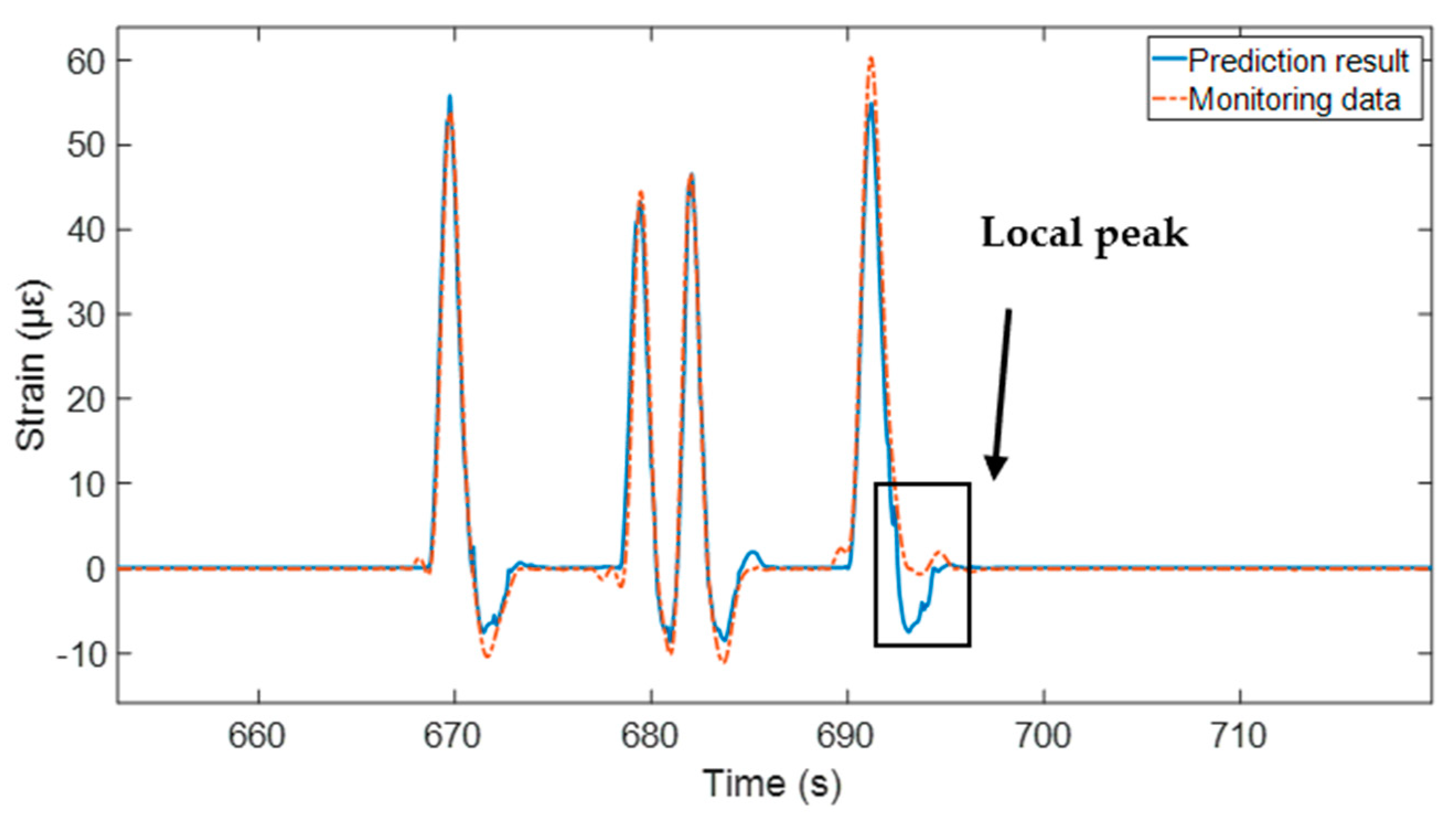
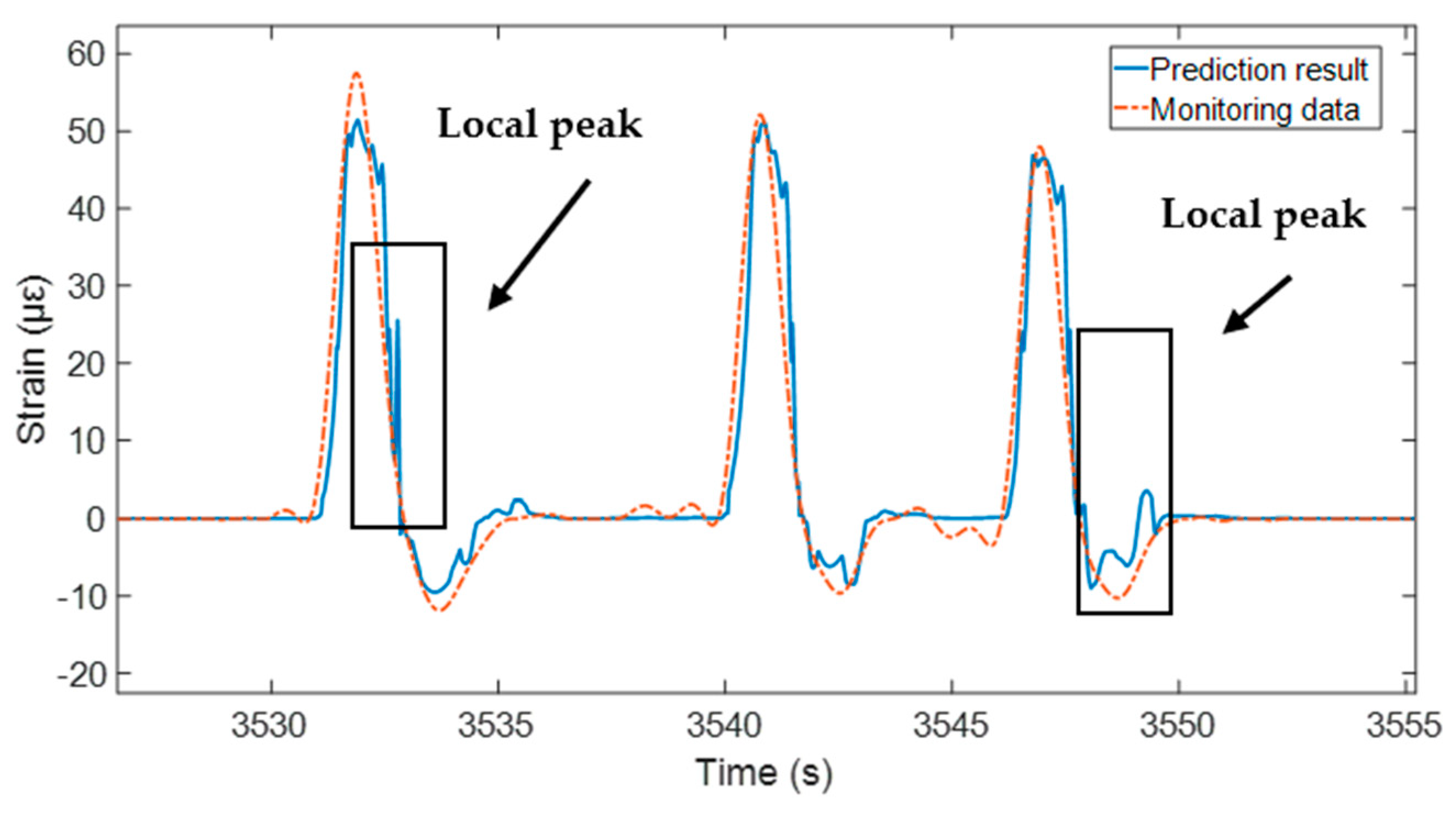
4.4. Result Discussion

Figure 18 illustrates the estimation of low-frequency bridge strain for the first case. It can be observed that, from 660 s to 700 s, there were multiple peaks in the time history of bridge strain, which indicates that multiple vehicles passed the target span in the monitoring period. The detailed conditions of these vehicles, including their number, mass, speed, and passing lanes, are unknown. However, as illustrated in Figure 18, the time instances corresponding to the peak amplitudes align closely between the estimated values and the actual monitoring data. Moreover, the highest estimated amplitudes correspond well with the periods when vehicles were passing, as observed in the monitoring data. This concurrence suggests that the proposed method effectively captured the relationship between the bridge’s strain and the vehicle interactions.

In certain time instances, the strain estimation could display a degree of imprecision, with the estimates exhibiting sudden peaks (indicated by rectangles in Figure 18) that were at odds with the more continuous curve observed in the monitoring data. This variance was thought to stem from the randomness inherent in batch processing and from measurement noise. Specifically, random batch processing does not ensure continuity in amplitudes between consecutive time points. Additionally, when the response amplitudes are relatively low, the method may not effectively separate the actual responses from noise, potentially leading to imperfect estimations. Nevertheless, these sudden peaks have a negligible effect on the estimated local peak values and the general shape of the time–history curve. It is conceivable that future modifications could be made to refine the model and yield a smoother estimation. However, such enhancements fall outside the scope of the current paper and will not be discussed further.

Additionally, the estimation results for the second case are depicted in Figure 19. Similar to Figure 18, the traffic conditions for the multiple passing vehicles in the second case are also known. Additionally, the temperatures for the training data set and the testing data set are different, which indicates a potential change in bridge-material stiffness. Figure 19 shows that the vehicle-passing periods, the highest amplitudes, and the time instances of these peaks, as observed in the monitoring data and the estimation results, match very well. It was inferred that temperature changes exert a negligible impact on the trained strain–vehicle interaction relationship. Furthermore, it is reasonable to assume that the primary mode shapes of the bridge remain stable over several months.

Another noteworthy aspect is the seven-month interval between the first and third monitoring days. The estimation results presented in Figure 19 indicate that the proposed method offers several advantages. Firstly, it eliminates the need to collect traffic condition or temperature data. Secondly, for long-term bridge health monitoring, it is practical to develop a long-term strain-interaction model using a minimal data set from a short monitoring period. This approach is especially beneficial for practical engineering applications, streamlining the process of bridge health assessment and reducing the resources required for data collection and analysis.

5. Conclusions

This paper introduces a physically guided machine learning approach to predicting low-frequency bridge responses at a particular cross-section, leveraging responses from other cross-sections under the influence of vehicle loading. The theoretical derivation of the physical characteristics of low-frequency bridge dynamics within a typical VBI system served as the foundation. Utilizing these physical insights, a time-independent BP-ANN was trained to estimate the time-series of low-frequency bridge responses. The proposed method was rigorously validated through a combination of numerical simulations and field experiments. The analysis led to the following key conclusions:

(1)

A theoretical analysis established that, for typical highway VBI systems, the commonly employed “quasi-static” approach to bridge responses closely approximates low-frequency responses, which are primarily dictated by the driving force modes. More significantly, the target strain–vehicle interaction relationship is time-independent. Specifically, the transfer matrix is solely dependent on the bridge’s mode shapes, and it remains constant across varying temperature and traffic conditions.

(2)

Finite element simulations were initially conducted to validate the physical characteristics of the transfer matrix. It was confirmed that the transfer matrix remains stable under fluctuating traffic conditions, including variations in vehicle mass, quantity, and speed. Furthermore, the robustness of the proposed method was demonstrated through tests involving artificially introduced noise in the simulation data.

(3)

In the field tests, the proposed method was validated across two scenarios. Despite varying and unknown traffic conditions and temperatures, the method exhibited excellent performance. The estimated low-frequency responses were found to align well with the monitoring data. Additionally, it was demonstrated that the proposed method has the potential to construct an effective estimation model for long-term monitoring, utilizing a small data set collected over a short monitoring period.

Compared to previous studies, this novel approach adeptly overcomes the challenges associated with extracting modal information from low-frequency responses. Moreover, it effectively circumvents the difficulties of obtaining comprehensive traffic and temperature data, which are essential for accurate structural health assessments. Consequently, we believe this method is poised to be highly applicable in real-world engineering scenarios.

It is important to note that the current study focuses solely on linear bridge structures. The applicability of this method to large-span bridges with significant nonlinear dynamics or bridges that have been potentially damaged and exhibit nonlinear behavior has yet to be determined. Specifically, traffic conditions and temperature may impact the modal characteristics of these nonlinear structures. Therefore, it is imperative to consider these factors in our analyses. These considerations are among the areas we intend to investigate more deeply in our future research.

References

1. Tian, Y.; Xu, Y.; Zhang, D.; Li, H. Relationship Modeling between Vehicle-Induced Girder Vertical Deflection and Cable Tension by BiLSTM Using Field Monitoring Data of a Cable-Stayed Bridge. Struct. Control Health Monit. 2021, 28, e2667. [Google Scholar] [CrossRef]
2. Oh, B.K.; Yoo, S.H.; Park, H.S. A Measured Data Correlation-Based Strain Estimation Technique for Building Structures Using Convolutional Neural Network. Integr. Comput. Aided Eng. 2023, 30, 395–412. [Google Scholar] [CrossRef]
3. Lu, L.-J.; Zhou, H.-F.; Ni, Y.-Q.; Dai, F. Output-Only Modal Analysis for Non-Synchronous Data Using Stochastic Sub-Space Identification. Eng. Struct. 2021, 230, 111702. [Google Scholar] [CrossRef]
4. Dosiek, L.; Zhou, N.; Pierre, J.W.; Huang, Z.; Trudnowski, D.J. Mode Shape Estimation Algorithms under Ambient Conditions: A Comparative Review. IEEE Trans. Power Syst. 2013, 28, 779–787. [Google Scholar] [CrossRef]
5. Poncelet, F.; Kerschen, G.; Golinval, J.-C.; Verhelst, D. Output-Only Modal Analysis Using Blind Source Separation Techniques. Mech. Syst. Signal Process 2007, 21, 2335–2358. [Google Scholar] [CrossRef]
6. Zhou, W.; Chelidze, D. Blind Source Separation Based Vibration Mode Identification. Mech. Syst. Signal Process 2007, 21, 3072–3087. [Google Scholar] [CrossRef]
7. Xiao, F.; Sun, H.; Mao, Y.; Chen, G.S. Damage Identification of Large-Scale Space Truss Structures Based on Stiffness Separation Method. Structures 2023, 53, 109–118. [Google Scholar] [CrossRef]
8. Xiao, F.; Yan, Y.; Meng, X.; Mao, Y.; Chen, G.S. Parameter Identification of Multispan Rigid Frames Using a Stiffness Separation Method. Sensors 2024, 24, 1884. [Google Scholar] [CrossRef]
9. Gulgec, N.S.; Takáč, M.; Pakzad, S.N. Structural Sensing with Deep Learning: Strain Estimation from Acceleration Data for Fatigue Assessment. Comput.-Aided Civ. Infrastruct. Eng. 2020, 35, 1349–1364. [Google Scholar] [CrossRef]
10. Xu, W.; Shi, X. Machine-Learning-Based Predictive Models for Punching Shear Strength of FRP-Reinforced Concrete Slabs: A Comparative Study. Buildings 2024, 14, 2492. [Google Scholar] [CrossRef]
11. Cheng, M.-C.; Bonopera, M.; Leu, L.-J. Applying Random Forest Algorithm for Highway Bridge-Type Prediction in Areas with a High Seismic Risk. J. Chin. Inst. Eng. 2024, 47, 597–610. [Google Scholar] [CrossRef]
12. Li, S.; Liang, Z.; Guo, P. A FBG Pull-Wire Vertical Displacement Sensor for Health Monitoring of Medium-Small Span Bridges. Measurement 2023, 211, 112613. [Google Scholar] [CrossRef]
13. Hidehiko, S.; Kosaku, K.; Chitoshi, M. Simplified Portable Bridge Weigh-in-Motion System Using Accelerometers. J. Bridge Eng. 2018, 23, 04017124. [Google Scholar] [CrossRef]
14. Breccolotti, M.; Natalicchi, M. Bridge Damage Detection through Combined Quasi-Static Influence Lines and Weigh-in-Motion Devices. Int. J. Civ. Eng. 2022, 20, 487–500. [Google Scholar] [CrossRef]
15. Zhao, H.; Uddin, N.; O’Brien, E.J.; Shao, X.; Zhu, P. Identification of Vehicular Axle Weights with a Bridge Weigh-in-Motion System Considering Transverse Distribution of Wheel Loads. J. Bridge Eng. 2014, 19, 04013008. [Google Scholar] [CrossRef]
16. Yu, E.; Wei, H.; Han, Y.; Hu, P.; Xu, G. Application of Time Series Prediction Techniques for Coastal Bridge Engineering. Adv. Bridge Eng. 2021, 2, 6. [Google Scholar] [CrossRef]
17. Hochreiter, S.; Jürgen, S. Long short-term memory. Neural Comput. 1997, 9, 1735–1780. [Google Scholar] [CrossRef]
18. Albawi, S.; Bayat, O.; Al-Azawi, S.; Ucan, O.N.; Lefevre, E. Social Touch Gesture Recognition Using Convolutional Neural Network. Intell. Neurosci. 2018, 2018, 6973103. [Google Scholar] [CrossRef]
19. Goodfellow, I.; Pouget-Abadie, J.; Mirza, M.; Xu, B.; Warde-Farley, D.; Ozair, S.; Courville, A.; Bengio, Y. Generative Adversarial Networks. Commun. ACM 2020, 63, 139–144. [Google Scholar] [CrossRef]
20. Zhao, H.; Ding, Y.; Li, A.; Sheng, W.; Geng, F. Digital Modeling on the Nonlinear Mapping between Multi-Source Monitoring Data of in-Service Bridges. Struct. Control Health Monit. 2020, 27, e2618. [Google Scholar] [CrossRef]
21. Xin, J.; Zhou, C.; Jiang, Y.; Tang, Q.; Yang, X.; Zhou, J. A Signal Recovery Method for Bridge Monitoring System Using TVFEMD and Encoder-Decoder Aided LSTM. Measurement 2023, 214, 112797. [Google Scholar] [CrossRef]
22. Wang, Z.; Wang, Y. Bridge Weigh-in-motion Through Bidirectional Recurrent Neural Network with Long Short-term Memory and Attention Mechanism. Smart Struct. Syst. 2021, 27, 241–256. [Google Scholar]
23. Li, Y.; Ni, P.; Sun, L.; Zhu, W. A Convolutional Neural Network-Based Full-Field Response Reconstruction Framework with Multitype Inputs and Outputs. Struct. Control Health Monit. 2022, 29, e2961. [Google Scholar] [CrossRef]
24. Pamuncak, A.P.; Salami, M.R.; Adha, A.; Budiono, B.; Laory, I. Estimation of Structural Response Using Convolutional Neural Network: Application to the Suramadu Bridge. Eng. Comput. 2021, 38, 4047–4065. [Google Scholar] [CrossRef]
25. Du, B.; Wu, L.; Sun, L.; Xu, F.; Li, L. Heterogeneous Structural Responses Recovery Based on Multi-Modal Deep Learning. Struct. Health Monit. 2023, 22, 799–813. [Google Scholar] [CrossRef]
26. Zhang, H.; Xu, C.; Jiang, J.; Shu, J.; Sun, L.; Zhang, Z. A Data-Driven Based Response Reconstruction Method of Plate Structure with Conditional Generative Adversarial Network. Sensors 2023, 23, 6750. [Google Scholar] [CrossRef]
27. Zhuang, Y.; Qin, J.; Chen, B.; Dong, C.; Xue, C.; Easa, S.M. Data Loss Reconstruction Method for a Bridge Weigh-in-Motion System Using Generative Adversarial Networks. Sensors 2022, 22, 858. [Google Scholar] [CrossRef]
28. Fan, G.; Li, J.; Hao, H.; Xin, Y. Data Driven Structural Dynamic Response Reconstruction Using Segment Based Generative Adversarial Networks. Eng. Struct. 2021, 234, 111970. [Google Scholar] [CrossRef]
29. Yang, Y.B.; Li, Y.C.; Chang, K.C. Constructing the Mode Shapes of a Bridge from a Passing Vehicle: A Theoretical Study. Smart Struct. Syst. 2014, 13, 797–819. [Google Scholar] [CrossRef]
30. Yang, Y.B.; Lin, C.W. Vehicle—Bridge Interaction Dynamics and Potential Applications. J. Sound Vib. 2005, 284, 205–226. [Google Scholar] [CrossRef]
31. Biggs, J.M. Introduction to Structural Dynamics; McGraw-Hill: New York, NY, USA, 1964. [Google Scholar]
32. Frýba, L. Vibration of Solids and Structures under Moving Loads; ICE Publishing: London, UK, 1999. [Google Scholar]
33. Huang, L.; Chen, J.; Tan, X. BP-ANN Based Bond Strength Prediction for FRP Reinforced Concrete at High Temperature. Eng. Struct. 2022, 257, 114026. [Google Scholar] [CrossRef]
34. Nurunnahar, S.; Talukdar, D.B.; Rasel, R.I.; Sultana, N. A Short Term Wind Speed Forcasting Using SVR and BP-ANN: A Comparative Analysis. In Proceedings of the 2017 20th International Conference of Computer and Information Technology (ICCIT), Dhaka, Bangladesh, 22–24 December 2017; pp. 1–6. [Google Scholar]
35. Huang, X.; You, Y.; Zeng, X.; Liu, Q.; Dong, H.; Qian, M.; Xiao, S.; Yu, L.; Hu, X. Back Propagation Artificial Neural Network (BP-ANN) for Prediction of the Quality of Gamma-Irradiated Smoked Bacon. Food Chem. 2024, 437, 137806. [Google Scholar] [CrossRef] [PubMed]
36. Al-Jarrah, R.; AL-Oqla, F.M. A Novel Integrated BPNN/SNN Artificial Neural Network for Predicting the Mechanical Performance of Green Fibers for Better Composite Manufacturing. Compos. Struct. 2022, 289, 115475. [Google Scholar] [CrossRef]
37. Yang, Y.-B.; Li, Y.C.; Chang, K.C. Effect of Road Surface Roughness on the Response of a Moving Vehicle for Identification of Bridge Frequencies. Interact. Multiscale Mech. 2012, 5, 347–368. [Google Scholar] [CrossRef]
38. Paultre, P.; Chaallal, O.; Proulx, J. Bridge Dynamics and Dynamic Amplification Factors—A Review of Analytical and Experimental Findings. Can. J. Civ. Eng. 1992, 19, 260–278. [Google Scholar] [CrossRef]
39. Dassault Systèmes. Abaqus 6.11 Analysis User’s Manual; Dassault Systemes Simulia Corporation: Providence, RI, USA, 2011. [Google Scholar]
40. Lu, X.; Kim, C.-W.; Chang, K.-C. Finite Element Analysis Framework for Dynamic Vehicle-Bridge Interaction System Based on ABAQUS. Int. J. Str. Stab. Dyn. 2020, 20, 2050034. [Google Scholar] [CrossRef]
41. Lei, X.; Sun, L.; Xia, Y. Lost Data Reconstruction for Structural Health Monitoring Using Deep Convolutional Generative Adversarial Networks. Struct. Health Monit. 2021, 20, 2069–2087. [Google Scholar] [CrossRef]
42. Xia, Y.; Lei, X.; Wang, P.; Liu, G.; Sun, L. Long-Term Performance Monitoring and Assessment of Concrete Beam Bridges Using Neutral Axis Indicator. Struct. Control Health Monit. 2020, 27, e2637. [Google Scholar] [CrossRef]
43. MATLAB. Signal Processing Toolbox (Version R2022a). MathWorks. Available online: https://www.mathworks.com/help/signal/ref/highpass.html#mw_dcf4bbd2-1e29-4f0f-819f-39d872f77a14_seealso (accessed on 30 August 2024).
Figure 1. A typical, simple VBI system.
Buildings 14 02995 g001
Figure 2. Responses corresponding to the first and second modes at three cross-sections. (a) First-mode responses; (b) second-mode responses; (c) summation of the first- and second-mode responses (left column: 1/4-beam responses; middle column: mid-beam responses; right column: 3/4-beam responses).
Buildings 14 02995 g002
Figure 3. Comparison between responses at three locations on the beam. (The “double arrow” denotes the observed time lag.)
Buildings 14 02995 g003
Figure 4. Artificial neuron unit [33].
Buildings 14 02995 g004
Figure 5. ANN structure for responses’ estimation (NS-1, …, and NS-m represent the input data from the m-th cross-sections).
Buildings 14 02995 g005
Figure 6. Finite element model for the simple VBI system built with ABAQUS 2020 (left and right edge nodes are marked in red).
Buildings 14 02995 g006
Figure 7. Comparison of mid-span displacement with different mesh densities.
Buildings 14 02995 g007
Figure 8. Cases for validation. (a) Reference; (b) high-speed; (c) light-mass; and (d) dual vehicles.
Buildings 14 02995 g008
Figure 9. Vertical displacement time history at three cross-sections in four cases. (Dashed line: the time instance when the largest displacement occurs on each curve. The left dashed line corresponds to the 1/4 beam. The middle dashed line corresponds to the 1/2 beam, and the right dashed line corresponds to the 3/4 beam). (a) Reference case; (b) high-speed case; (c) light-mass case; and (d) dual vehicles.
Buildings 14 02995 g009
Figure 10. Comparison of vertical displacement time history at 1/4 of the beam between the estimation and simulation results. (a) Reference case; (b) high-speed case; (c) light-mass case; and (d) double-vehicle case (solid curve: estimated displacement; dashed line curve: simulation results).
Buildings 14 02995 g010
Figure 11. Comparison between the estimation result with BP-ANN and the simulation result with white noise.
Buildings 14 02995 g011
Figure 12. Target Bridge and the SHM system. (a) Fuchang Bridge [41]; (b) SHM system [42].
Buildings 14 02995 g012
Figure 13. A piece of typical strain monitoring data. (Rectangle marked data in (a) is zoomed in on and illustrated as (b), and Rectangle marked data in (b) is zoomed in on and illustrated as (c)).
Buildings 14 02995 g013
Figure 14. Time-lag phenomenon in the strain time history between different cross-sections. (Triangle marks denote the highest amplitude for each strain time–history curve.)
Buildings 14 02995 g014
Figure 15. Strain time histories at three cross-sections with multiple passing vehicles.
Buildings 14 02995 g015
Figure 16. High-frequency bridge strain at 02-S01 under vehicular loading in August and October. (a) Monitoring data in August; (b) monitoring data in October. (Left column: strain time history; right column: frequency spectrum.)
Buildings 14 02995 g016
Figure 17. Training and testing data sets in the case study. (a) First case; (b) second case.
Buildings 14 02995 g017
Figure 18. Comparison for low-frequency strain at 02-S01 (First case).
Buildings 14 02995 g018
Figure 19. Comparison for low-frequency strain at 02-S01 (Second case).
Buildings 14 02995 g019