2. ECB and the Financial Crisis
Since the introduction of the Euro in 1999, the European Central Bank (ECB) has been responsible for the monetary policy in the European currency area. Article 127 of the Consolidated Treaty on the Functioning of the European Union defines the mandate of the ECB: “The primary objective of the European Systems of Central Banks … shall be to maintain price stability.” (see Conference of the Representatives of the Governments of the Member States [
1]). Therefore, the Governing Council of the ECB aims to keep inflation below, but close to 2%. Thus, the monetary policy of the ECB is only required to price stability. Contrary to this, the mandate of the Federal Reserve (Fed) for example is defined in a broader way. In addition to price stability the Fed is required to support the development of the labor market (see for example Pollard [
2] and Thorbecke [
3]). In relation to their mandate the members of the Governing Council of the ECB focus on stable inflation expectations to achieve price stability.
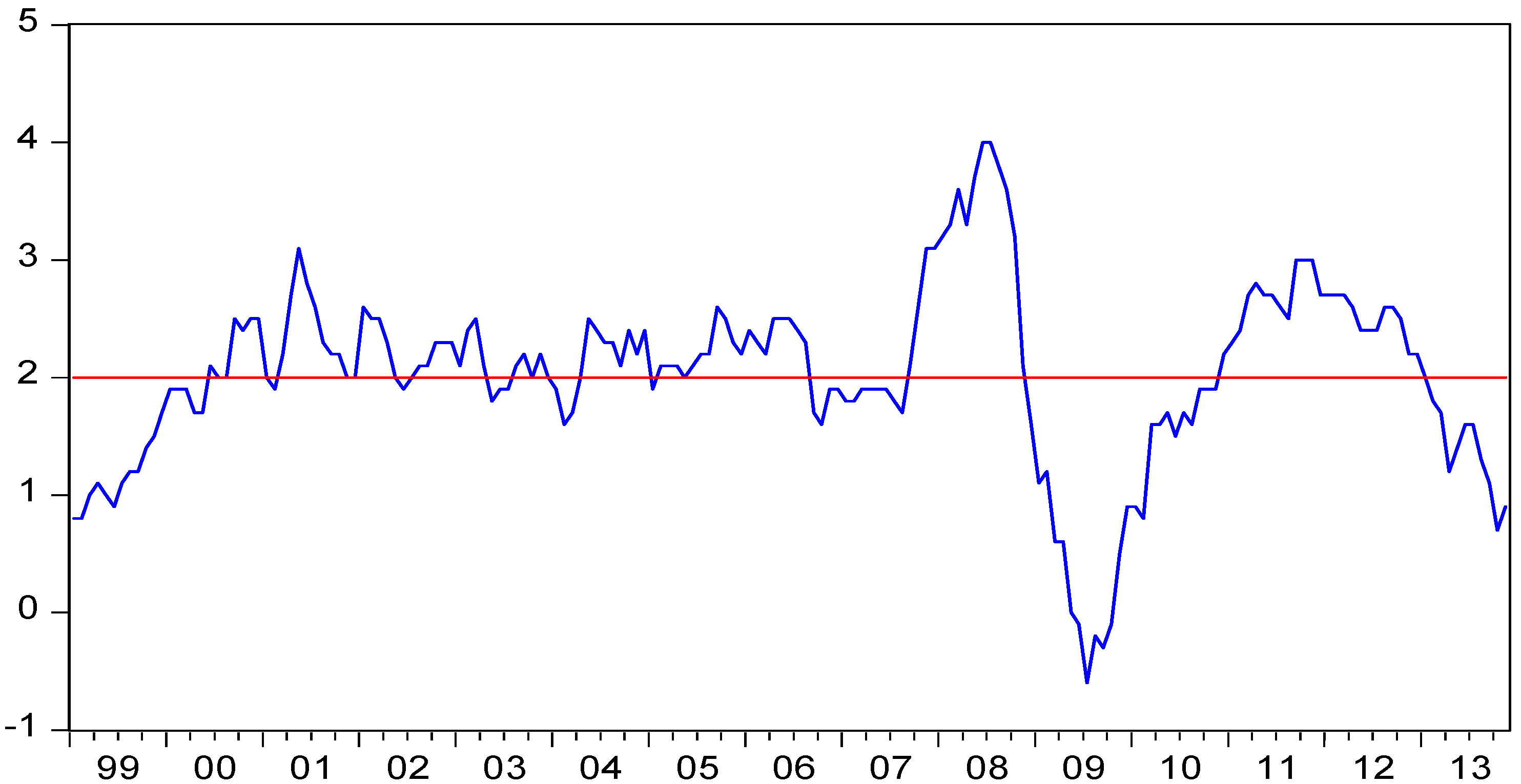
Since the start of the ECB in 1999 the inflation rate in the Eurozone, measured by the harmonized consumer price index, is roughly 2%. Therefore, it seems that—until now—the ECB has reached its aim of stable prices, even if the increase of the harmonized consumer price index has been higher than 2% in some times (see
Figure 1).
The development of inflation can be influenced by the interest rate level. Short-term interest rates are directly controlled by the monetary policy rates. Higher rates typically go hand in hand with higher market interest rates and vice versa. This is especially true for the short end of the yield curve. Ellingsen and Söderström [
4] deliver a very comprehensive analysis dealing with this phenomenon. Moreover, this connection affects inflation expectations and inflation rates in an indirect way. To summarize it with a short rule: In times of high inflation rates the Central Bank has to increase their interest rates, which results in higher short-term interest rates and puts a brake on the economic development. This typically leads to lower price pressure. If the inflation rates are low or even too low, the central bank has to reduce their interest rates, which lowers the short-term interest rates and therefore can fuel the economic situation and leads to increasing inflation rates in the near future. Putting it the other way round, there does exist a relationship between economic variables as well as monetary policy rates. In times of economic as well as financial crisis this might make central bankers’ interest rate moves more predictable. This could especially be true if one assumes that the central banks’ decision makers follow a certain rule.
Figure 1.
European inflation rate January 1999–November 2013 vs. 2% inflation target in %; Source: EUROSTAT.
Figure 1.
European inflation rate January 1999–November 2013 vs. 2% inflation target in %; Source: EUROSTAT.
In this context one can refer to the well-known policy rule by Taylor [
5]:
In Equation (1)
r represents the federal funds rate whereas the rate of inflation for over the previous four quarters is expressed by
p. Finally
y represents the percent deviation of real GDP from a predetermined target. A lot of effort has been spent by various academic researchers as well as practitioners to understand and forecast the monetary policy makers’ decision with the help of relevant economic variables. See for example Clarida
et al. [
6], Clarida
et al. [
7] and Ullrich [
8]. For a discussion whether the ECB’s central bankers rely on the Taylor rule during the current crisis see Belke and Klose [
9] as well as Gerdesmeier and Roffia [
10].
Due to the fact that the monetary policy rates influence short-term interest rates and therefore have direct and indirect connection to future economic development, including growth and prices but also asset price development, the action of central banks is of high interest to the market participants. Therefore the forecast of future monetary policy action and especially the forecast of future development of short-term interest rates are of high importance, too.
Since the financial crisis the ECB has to think about this connection more serious. The financial crisis lead to deep recessions in most of the member states of the Eurozone. Following Eurostat data in 2009 real GDP shrank by −4.4% in the currency area. In Germany, the biggest economy of the Eurozone, the GDP reduction was even harder with about −5.1%. In France and Italy real GDP shrank by −3.1% and −5.5%. Therefore the Central Bank had to react and lowered their interest rates efficiently and drastically. While the main refinancing rate was at 4.25% in July 2008 the Governing Council lowered this rate down to 1.00% in mid-2009. Even if the harmonized consumer price index increased by 4.0% in July 2008, the economic crisis in the Eurozone indicated lower price pressure for the months to come. In early 2009, the inflation rate in the currency area measured by the harmonized consumer price index fell down to 1.1%.
To bring more transparency into the decision of the Governing Council the ECB currently discusses the publication of minutes, like other Central Banks already do. Proponents argue that the publication of minutes would improve the understanding of the monetary policy decisions. Maybe it would improve the quality of short-term interest rates forecasts, due to better hints regarding the future monetary policy. Opponents argue that minutes would reduce the independence of the ECB and its monetary policy. Belke [
11], for example, raised the question whether central bankers could face more political pressure if their votes become public. To improve the level of transparency the ECB already implemented a “Forward Guidance” in July 2013. As ECB president Mario Draghi mentioned in the corresponding press conference “… the Governing Council expects the key ECB interest rates to remain at present or lower levels for an extended period of time” (see Draghi [
12]). A current discussion on central bankers’ transparency as well as forward guidance is delivered by El-Erian [
13] as well as Fawley and Neely [
14]).
The motives and reactions of the central bankers to the current financial crisis raise the question whether it has become more difficult or even easier to predict their interest moves and hence the market reactions respectively the short end of the yield curve. Because of this we will evaluate professional forecasters’ performance in predicting the three-month EURIBOR later in this paper. Before that, in
Section 3 we will deliver a short review of the literature relevant to financial market forecasts.
3. Literature Review
For decades, the quality of financial market forecasts has been in the focus of interest both of the finance industry and academics. The uncertainty of the future developments of short- and long-term interest rates, FX and equity markets leads to a major source of risks for market participants but may also lead to substantial revenues if anticipated correctly. Not surprisingly, financial market professionals put a lot of effort into their predictions, which are also demanded by a large proportion of the financial industry’s customers. Not surprisingly, the precision respectively usefulness of financial market forecasts has to be assessed constantly.
Today we are able to look back to almost a century of research dealing with the evaluation of financial market forecasts. One ground breaking work of Theil [
15] can be dated back almost 60 years, for example. Since then, researchers have evaluated professional forecasters’ performance in a broad spectrum of financial market times series ranging from equity markets (see for example Guedj and Bouchaud [
16] as well as Spiwoks and Hein [
17] and Bessler and Stanzel [
18]), foreign exchange markets (see for example Lai [
19] and more recently Della Corte
et al. [
20]) as well as interest rate forecasts (see for example Friedman [
21], Belongia [
22] and more recently Gubaydullina, Hein and Spiwoks [
23]).
The evaluation of interest forecasts for the German government bond market as well as the European short term interest rate is of high relevance for the focus of this paper. The usefulness of interest rate forecasts dealing with European and German government bond markets has been, for example, investigated by Chortareas, Jitmaneeroj and Wood [
24] as well as Schwarzbach
et al. [
25]. Spiwoks, Bedke and Hein [
26] did assess the accuracy of professional forecasts for the Swiss Bond market. Kunze, Kramer and Rudschuck [
27] investigated the performance of professional analysts forecasting the three-month EURIBOR and checked for dispersion within the survey forecasts due to financial crisis related uncertainty and therefore this work is of high relevance for the focus of this paper. Within their study the authors did focus on the possibility to use the dispersion within the individual forecasts as a financial crisis indicator whereas within this paper we focus on crisis related quality changes of professional forecasts. For the literature of empirical assessments of interest rate forecasts especially for the three-month interest rate in Germany the work of Spiwoks, Bedke and Hein [
28] is of high relevance. Bedke, Spiwoks and Hein [
29] additionally did focus on US interest rates.
Besides the evaluation of interest rate forecasts, analyzing the structural breaks in the long run relationship between interest rates triggered by financial crisis is extremely important in this context. See for example Basse, Friedrich and Kleffner [
30] as well as Gruppe and Lange [
31] and Basse [
32] for a detailed investigation of the impacts on long run relationships caused by the European sovereign debt crisis. As Brand, Buncic and Turunen [
33] as well as Kunze, Kramer and Rudschuck [
27] have mentioned the ECB’s monetary policy and the communication thereof do both influence the term structure of interest rates. This is especially true for the short term interest rates like the three-month EURIBOR, which we investigate in this paper. To put it somewhat differently, the European central bankers’ reactions to the financial market turbulences as well as the European sovereign debt crisis must have a substantial impact on the three-month EURIBOR. This raises the question which we want to answer within our empirical section: Did the European Debt Crisis make it harder or probably even easier do predict the three-month EURIBOR?
4. Data and Methodology
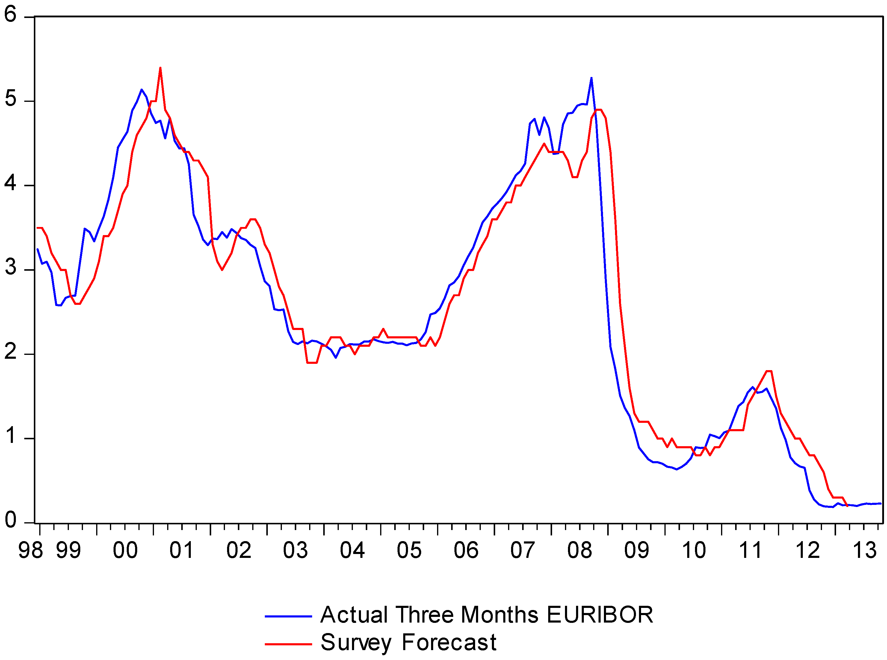
To find evidence for crisis related changes in the performance of forecasting the three-month EURIBOR by professional financial analysts we evaluate the survey mean of the three months ahead forecast published monthly by Consensus Economics Inc. To be more precise, the three months forecast in fact rather is a four months prediction. This is true because Consensus Economics asks for forecast contribution by the professional analysts at the beginning of the reporting month. To avoid any confusion we refer to the forecast time series as “survey forecast”. Our data sample of the survey forecasts as well as the three-month EURIBOR ranges from December 1998 until March 2013 and because of that incorporates a significant part of the Global Financial as well as European Currency Crisis. The underlying time series can be seen in
Figure 2. It seems to be more than obvious that both time series are non-stationary.
Because of that and to avoid any spurious results we start our empirical analysis by testing the three-month EURIBOR as well as the survey forecast for unit roots using the widely known PP-Test. The test results are presented in
Table 1 and
Table 2.
Figure 2.
Actual three-month EURIBOR vs. survey forecastsin %; Source: EUROSTAT/consensus economics.
Figure 2.
Actual three-month EURIBOR vs. survey forecastsin %; Source: EUROSTAT/consensus economics.
Table 1.
PP-test three-month EURIBOR.
Table 1.
PP-test three-month EURIBOR.
| Null Hypothesis: Three-Month EURIBOR has a unit root | |
| Exogenous: Constant | | |
| Bandwidth: 8 (Newey-West automatic) using Bartlett kernel |
| | | | Adj. t-Stat | Prob.* |
| Phillips-Perron test statistic | −1.205573 | 0.6718 |
| Test critical values: | 1% level | | −3.467205 | |
| | 5% level | | −2.877636 | |
| | 10% level | | −2.575430 | |
Table 2.
PP-Test Survey Forecast.
Table 2.
PP-Test Survey Forecast.
| Null Hypothesis: Survey Forecast has a unit root |
| Exogenous: Constant | | |
| Bandwidth: 8 (Newey-West automatic) using Bartlett kernel |
| | | | | |
| | | | Adj. t-Stat | Prob.* |
| Phillips-Perron test statistic | −1.197263 | 0.6753 |
| Test critical values: | 1% level | | −3.468749 | |
| | 5% level | | −2.878311 | |
| | 10% level | | −2.575791 | |
Both for the three-month EURIBOR and the survey forecast, the null hypothesis may not be rejected. Performing the PP-Test for the first differences of both time series leads to the rejection of a unit root and hence shows that both time series are integrated of order one (the test results will not be resulted here in order to preserve space).
To further assess the effect of financial crisis events on forecast performance of financial market professionals we first introduce simple but widely acknowledged forecast accuracy measure, the Theil’s U statistic introduced by Theil (see Theil [
15] and [
34]). See also Hynmdan [
35] for the application of the Theil’s U as a measure for forecast evaluation. The statistic can be defined as follows:
where
it is the actual value of the three-month EURIBOR at time t. T is the number of data points, h is the forecast horizon (
h = 4 months) and
ît is the value of the survey forecast at
t. Finally
it−h is the naïve forecast (
i.e., the value of i
t four months ago).
To analyze the relative forecast performance we additionally follow the representation of Andres and Spiwoks [
36] and use the following version of the Theil index defined below.
where
Ft is the relative forecasted change of the interest rate and
At is the relative actual change of the interest rate. To avoid any confusion we will refer to this measure as
Ur.
The interpretation of both statistics is straightforward. U’s lower boundary is zero. A value of U < 1 indicates that a forecast is better than a naïve forecast. U > 1 signals that forecast do not perform better than a naïve forecast.
To be able to quantify changes in the forecast performance we test for structural breaks within the relationship between the EURIBOR and the survey forecasts using the Quandt-Andrews-Test. First of all we estimate the simple following simple linear regression model using the actual interest
it as the dependent and the forecast
ît and the one-month lag of
it as the independent variable. Because we are dealing with non-stationary variables we estimate the model on first differences. α, β
1 and β
2 are the relevant estimated coefficients and
ut is the error term:
After estimating this simple linear regression model we test this relationship for structural breaks and their timing using the breakpoint testing procedure proposed by Quandt-Andrews (see for example Andrews [
37]). The attractiveness of the test in the context of this paper comes from the fact that no assumptions for possible break point dates have to be made in advance.
Finally—with the results from the Quandt-Andrews test (see Andrews [
37])—we will compare the forecasting performance of the survey forecast before and after the break point using the Theil-statistics outlined above.
5. Empirical Results
As outlined in the previous section we start our analysis with the estimation of a simple linear regression using the first differences if the actual interest rate (
it), the survey forecast (
ît) as well as the actual interest rate lagged by one month (
it−1). Our results are presented in the regression equation below. The
t-statistics for the estimated coefficients are reported in brackets.
Searching for structural breaks with unknown timing leads to the following results (
Table 3).
Table 3.
Quandt-Andrews breakpoint test.
Table 3.
Quandt-Andrews breakpoint test.
| Quandt-Andrews unknown breakpoint test |
| Null Hypothesis: No breakpoints within 15% trimmed data |
| Varying regressors: All equation variables |
| Equation Sample: 1999M02 2013M03 |
| Test Sample: 2001M04 2011M02 |
| Number of breaks compared: 119 |
| Statistic | Value | Prob. |
| Maximum LR F-statistic (2008M11) | 9.462575 | 0.0001 |
| Maximum Wald F-statistic (2008M11) | 28.38772 | 0.0001 |
| Exp LR F-statistic | 1.329651 | 0.0647 |
| Exp Wald F-statistic | 9.437692 | 0.0010 |
| Ave LR F-statistic | 1.626766 | 0.1190 |
| Ave Wald F-statistic | 4.880299 | 0.1190 |
We used the critical values calculated by Hansen [
38]. The interpretation of this test result is straightforward. There is strong evidence for a breakpoint within the relationship between the survey forecast and the actual interest rate. The timing of the breakpoint in November 2008 does not come as a surprise at all. Displaying the forecast errors (
i.e.,
ît–
it) in
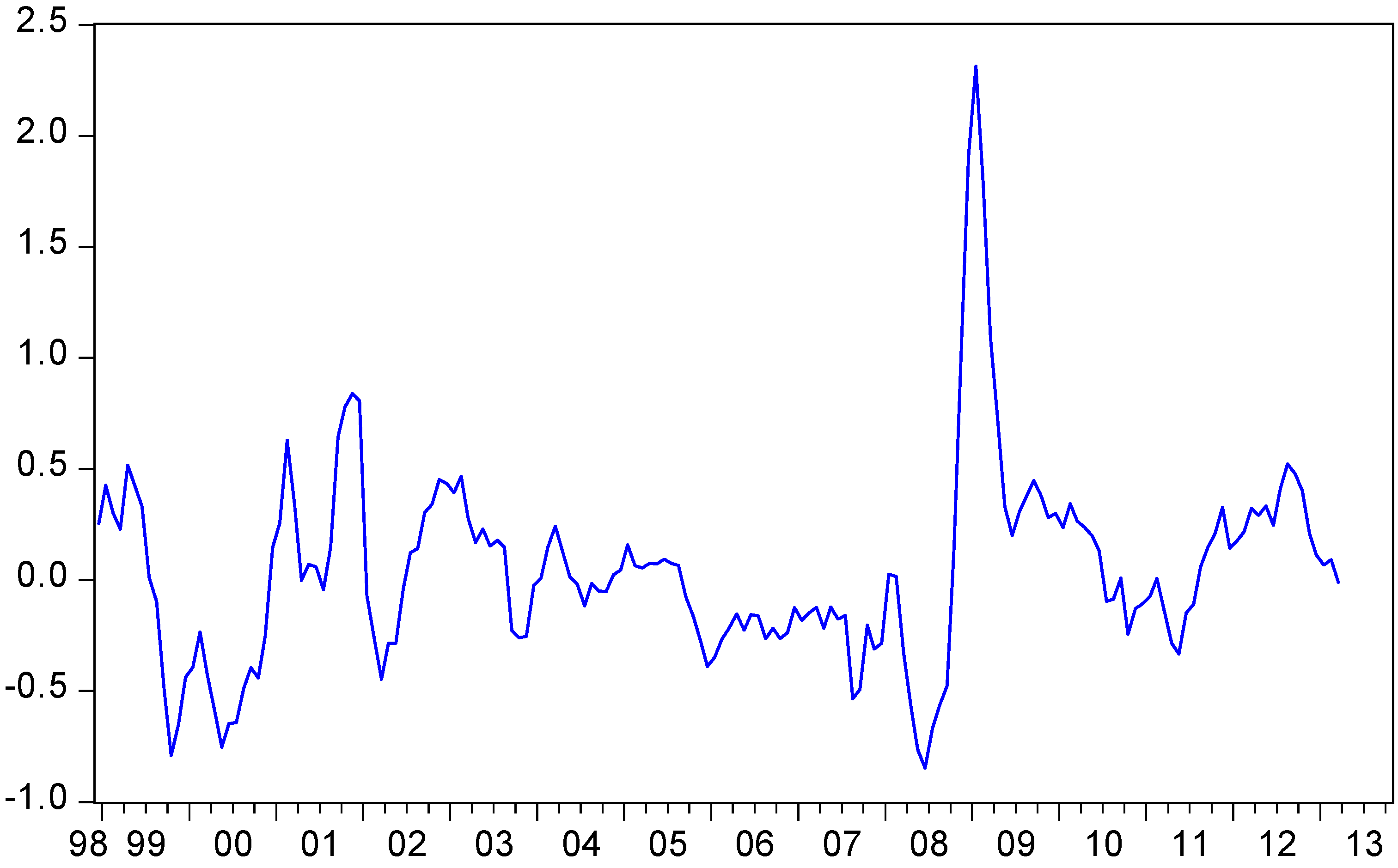
Figure 3 leads to a similar interpretation. Especially in 2008 the professional forecasters seem to have had difficulties anticipating the direction of the interest rate changes correctly. Examining
Figure 3 this is true for the rising EURIBOR preceding the sharp rise in late 2008, respectively early 2009. In 2008, professional forecasters failed to predict the surprising rate hike in July. As a consequence of rising oil prices and therefore temporarily higher inflation rates in the Eurozone the Central Bankers raised the interest rates by 25 basis points, which came as a surprise to most market participants. As a matter of fact, during that time the economic consequences of the financial crisis have already been quite obvious, which made the interest step even more surprising. With the banking and financial crisis having a much stronger than anticipated impact on the real economy in the Eurozone the ECB drastically lowered the benchmark interest rates in the remaining months of 2008 and the first quarter of 2009. These moves in turn have not been predicted by the professional analysts contributing to the Consensus Economics survey forecast either.
Figure 3.
Forecast Errors Three-Month EURIBOR Interest Rates in percentage points.
Figure 3.
Forecast Errors Three-Month EURIBOR Interest Rates in percentage points.
To further evaluate the potential changes in the analysts forecast accuracy we will finally focus on three time horizons: April 1999 until March 2013, April 1999 until November 2008 as well as December 2008 until March 2013. After applying the concepts given in the formulas (2) and (3) above we get the following results (
Table 4).
Table 4.
Result from Theil’s U and Theil’s Ur Analysis.
Table 4.
Result from Theil’s U and Theil’s Ur Analysis.
| Measure | 1999/04–2013/03 | 1999/04–2008/11 | 2008/12–2013/03 |
|---|
| Theil’s U | 0.7454545 | 0.8460556 | 0.6893854 |
| Theil’s Ur | 0.8711607 | 0.8262579 | 0.8834104 |
The findings are really interesting. The results from formula (2) indicate that after the breakpoint in November 2008 the professional analysts forecast performance may have improved. However, this interpretation might be dangerous because the lower value of 0.6893854 after the breakpoint stems more from an underperforming of the naïve forecast than from an improvement of the survey forecasts. This can also be seen from the error components before and after breakpoint. Up until November 2008 the sum of the squared error terms of the naïve respectively survey forecasts have been 0.1338553 respectively 0.1869983. After the break both error terms rose heavily (naïve forecast: 0.7194602, survey forecast: 0.3419251). Focusing on the relative forecast performance Ur leads us to a different conclusion with respect to crisis forecast performance. After the breakpoint the survey forecast’s Theil’s Ur presented in Equation (3) is slightly higher than before the structural break. However, we do not see that as evidence for a worsening of forecast performance. Summing up these results, it has to be stated that there does exist no evidence for neither a crisis related improvement nor a crisis related worsening of the forecast performance of professional forecasters. The stronger Theil’s U derived from the absolute errors reported in the table above stems rather from the weakness of the naïve forecast than from the strength of the survey forecast.


