1. Introduction
A landslide is a complex natural phenomenon [
1]. It is influenced by many geological environmental factors, such as topography, landform, geology, land use, and vegetation [
2]. A landslide is one of the most familiar and disastrous geological hazards with great destructiveness, which always poses a serious threat to human life, property, and living environment, and restricts human progress and development, especially when geological environments are increasingly affected by human engineering activities [
3]. Therefore, landslide prediction is of great significance for landslide prevention and control [
4,
5]. One of the greatest tasks of landslide disaster and risk mitigation is to prepare landslide susceptibility maps [
6].
With the development and progress of the geographic information system (GIS), its application in spatial analysis of landslides is becoming more and more popular. With proper use of GIS, most of the landslide susceptibility mapping methods can realize the automation of evaluation and standardization of data management technology, and enable us to build more efficient and accurate maps [
7,
8]. This is because these technologies can obtain, query, store, analyze, manipulate, and display a set of spatial and non-spatial data about landslide conditioning factors [
8,
9,
10]. Landslide susceptibility zoning mapping technology includes a variety of statistical techniques and statistical methods, including Dempster–Shafer [
11,
12,
13], entropy [
14,
15,
16], logistic regression [
17,
18,
19], certainty factors [
20,
21,
22], statistical index [
23,
24], analytic hierarchy process [
25,
26,
27], frequency ratio [
20,
28], weight of evidence [
29,
30,
31,
32], index of entropy [
20,
33], multivariate adaptive regression spline [
34,
35,
36], and evidential belief function [
37,
38,
39].
Landslide susceptibility mapping is a typical complex nonlinear problem in a large area of a landslide research area [
5]. Thus, the results obtained by statistical techniques and statistical methods may not be able to achieve satisfactory accuracy [
5,
40]. Later, many researchers proposed a large number of machine learning techniques for evaluating the susceptibility of landslides, which usually have high prediction accuracy and better performance in data-driven models, such as naive Bayes [
41,
42,
43], random forests [
2,
44,
45,
46], artificial neural networks [
47,
48,
49,
50], kernel logistic regression [
51,
52], support vector machine [
53,
54], and decision trees [
55,
56]. However, the performance of machine learning methods is generally influenced by the quality and quantity of training data, and the dependence on modeling parameters is very high [
5,
57]. So far, it is not clear which method is most suitable for landslide susceptibility mapping [
5].
In recent years, hybrid technology is considered to be more effective than single technology [
58]. In order to explore more reasonable and perfect research results, a variety of integrated algorithms have been developed for landslide susceptibility modeling [
6], such as adaptive neuro-fuzzy inference system [
59,
60], artificial neural networks-Bayes analysis [
61], and Evidential Belief Function-fuzzy logic [
62]. The important capability of the integrated model is that the method is more accurate in identification and greatly improves the prediction ability compared with the single machine learning model [
6].
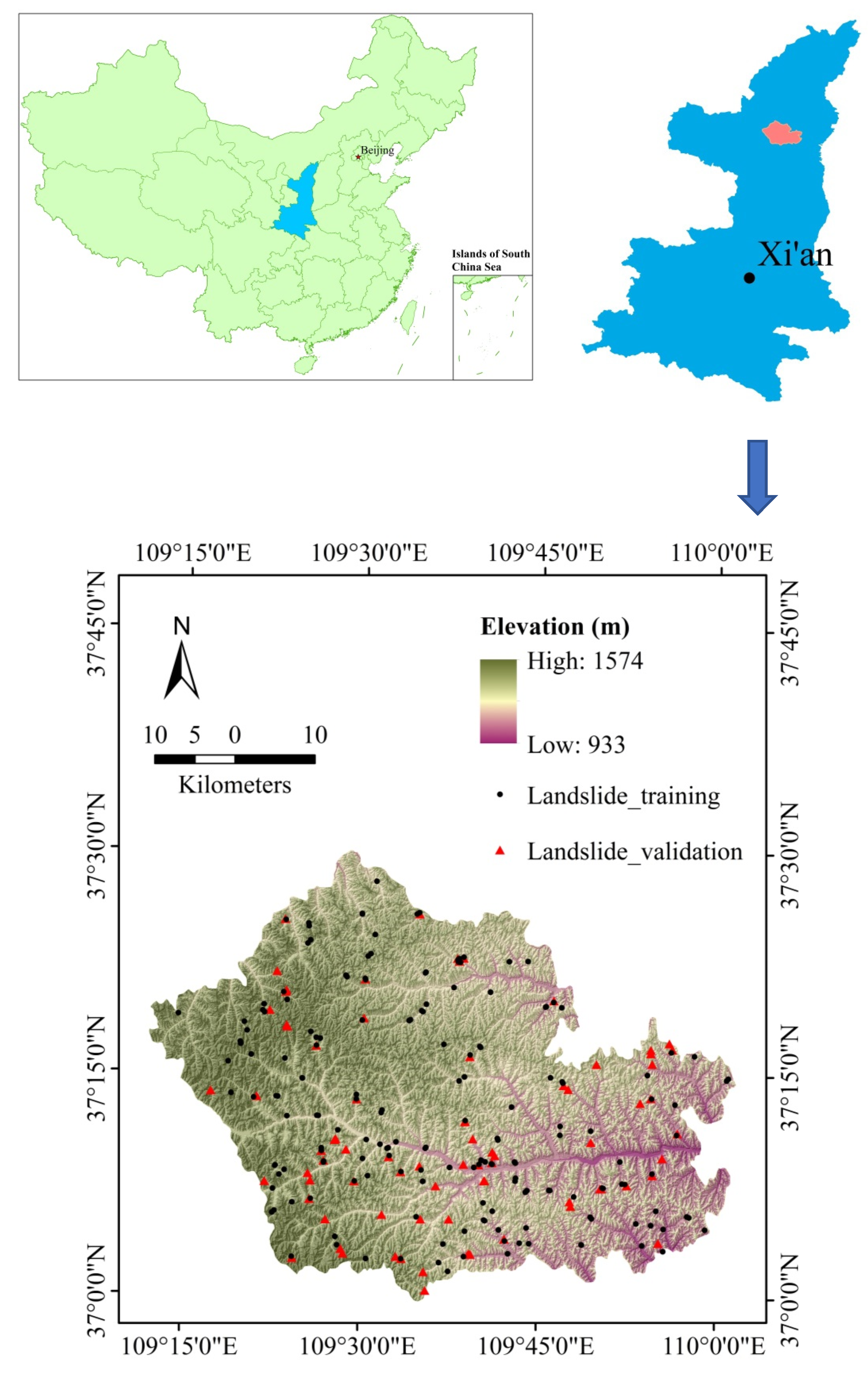
The purpose of this study is to propose and validate the ability and effect of ensemble techniques in landslide susceptibility modeling, and functional trees are selected as the base classifier to ensemble with bagging, rotation forest, and dagging models in Zichang County (China). Receiver operating characteristics (ROCs) and statistical parameters were used to evaluate and compare the overall performance of the four models.
3. Modeling Approach
The chapter included the illumination of five models, namely certainty factors, functional trees, bagging, rotation forest and dagging. The certainty factors model was used to express the correlation between landslide and conditioning factors, the functional trees model was used as a base classifier, the bagging, rotation forest, and dagging were used as ensemble algorithms.
3.1. Certainty Factors
The certainty factor (CF) belongs to a probability function, which was first proposed in 1990 [
66] and modified subsequently [
67]. The certainty factor can be expressed as [
68]:
where,
PPa is the conditional probability of landslide in class
a in study area A,
PPs is the prior probability of the total number of landslides in study area A.
The range of
CF is −1 to 1, the positive value indicates that the degree of certainty of landslide occurrence increases, while the negative value indicates that the degree of certainty of landslide occurrence decreases [
69,
70,
71].
3.2. Functional Trees
Functional trees (FT) are a combination of a discriminant function and multivariable decision tree through constructive induction [
72]. Functional trees use logistic regression functions to calculate the splitting of internal nodes (called oblique splitting) and estimation of leaves [
73,
74,
75]. FT learns the classification tree based on the attributes of leaf nodes, decision nodes or nodes and leaves [
38,
76]. The decision nodes are built while the trees are growing, while the functional leaves construct when the trees are pruning [
76]. Functional trees have the following three usage types: (1) the full functional tree using a regression model for internal nodes and leaves; (2) function tree internal-only uses the regression model for internal nodes; (3) functional tree leaves only use the regression model for leaves [
75,
76].
In the leaf logic regression function, the logic enhancement (iteration are weighted) of the least-squares function is determined for each output consisting of two classes [
77]. Among them, training datasets of D and
n samples (
,
) with
,
[
76].
is the input vector containing all landslide condition factors [
75,
76]; whereas
P(
A) is the probability prediction value of landslide occurrence;
is the coefficient of the
i component of the input vector
. The posterior probability
of the left ventricle is calculated as follows [
78]:
3.3. Bagging
Bagging is based on the concepts of bootstrapping and aggregating, which is used to obtain a more robust and accurate landslide model. Bagging is one of the most popular integration algorithms [
79]. The process of a bagging algorithm includes:
Firstly, the bootstrap samples
are randomly resampled from a training set (
,
), forming a set of training subsets, where,
,
(landslide, non-landslide) [
80]. Then, several models based on a classifier are constructed according to each subset,
is a classifier constructed from each guiding sample. All models based on classifier (
) are aggregated to generate the final model (
), where,
generates a combined classifier (
).
predicts the class label of a given instance
by calculating the votes using the following equation [
81]:
3.4. Rotation Forest
Rotation forest (RF) is a popular aggregation technique proposed by Rodriguez et al. [
82]. RF is an effective technique for improving weak classifiers [
83]. It uses principal component analysis (PCA), a multivariate technique used for analyzing large multivariate datasets, to reduce its dimensions [
84]. In this method, features are extracted from the learning (training) dataset and a base classifier is used to generate learning sub training dataset [
82].
For the use of RF: randomly divide the training dataset into D subsets, where D is the parameter of the algorithm, and construct the rotated sparse matrix by performing feature extraction for each subset. The classifier is based on the feature of a repeated matrix projection, and the result is obtained by combining the output of multiple classifiers [
84]. RF can be used with any basic classifier, and the feature extraction of each classifier retains all the features that promote variability [
84].
In the RF algorithm,
is the training sample set, and Y is the corresponding class label, that is used to consider landslides and non-landslides;
are the classifier in the set frame; and P is the set of landslide condition factors. The coefficients of the rotation matrix
are obtained by transformation and base classifier. Obtain
by rearranging
matrix [
84]:
For each sub training dataset extracted by the rotation matrix
, average grouping method is adopted to obtain the coefficients of each class in a given test sample [
85]:
where
is the maximum confidence specified on the class, classifier probability allocation
, and the
regression
[
85].
3.5. Dagging
Dagging is a well-known resampling integration technique originally proposed by Ting and Witten to generate many disjoint hierarchical folds from a dataset, and each data partition can be sent separately to the basic classifier [
86]. The final forecast is based on a majority vote [
86]. The main principle is to use a majority vote to combine multiple classifiers to improve the prediction accuracy of the basic classifier [
86].
For a given training dataset, which has
n samples, the dagging algorithm constructs M datasets (M is a free parameter) from the original training dataset [
87]. Each dataset contains
n samples [
87], and no two datasets have the same sample. A basic classifier is trained for each dataset to build a classification model [
87]. Therefore, the M dataset can be summarized into M classification models [
86,
87].
4. Results
This section consists of the detailed description of the results of the present study, which includes the following four sections: (1) the correlation between landslide and conditioning factors, and then the CF values are used as input to weight the classes of conditioning factors; (2) selection of landslide conditioning factors that are positive to the modeling process; (3) application of four hybrid models and generate landslide susceptibility maps; and (4) validation and comparison of models using ROC and Chi-squared methods.
4.1. Correlation Analysis of Landslide and Conditioning Factors Using the CF Method
The landslide density at each class was calculated by combining each thematic map and landslide inventory map. Meanwhile, this paper summarizes the spatial relationship between the landslides and conditioning factors using the CF method (
Table 2). According to the calculation results in
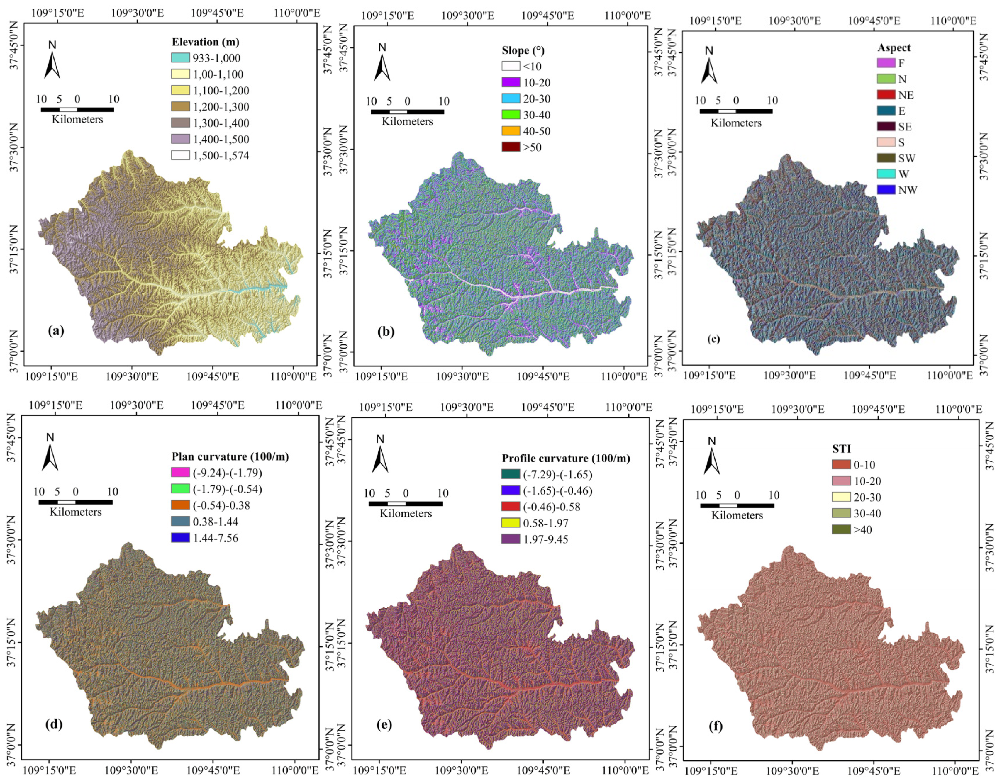
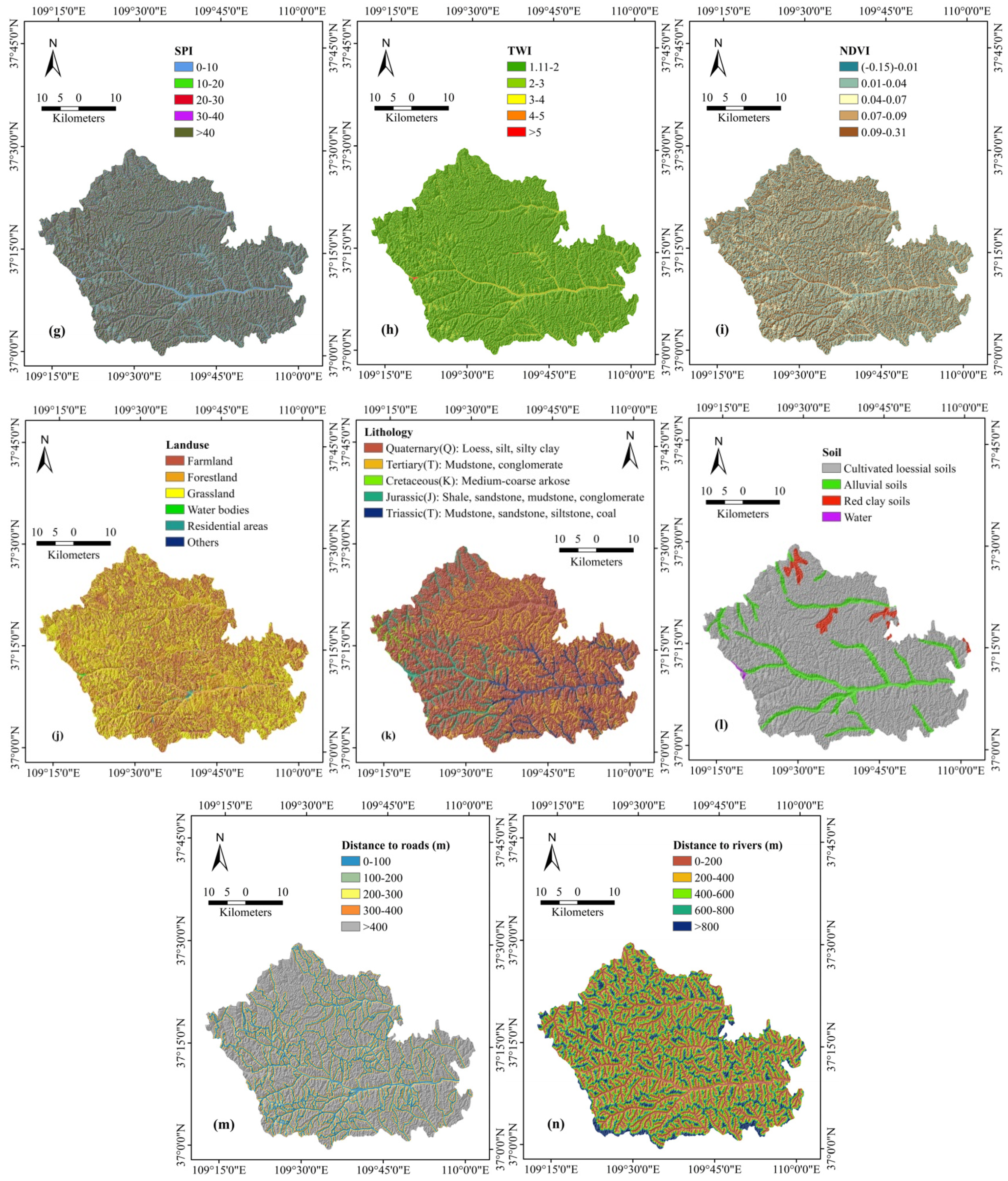
Table 2, the highest CF value (0.661) is found in the elevation category of 1500–1574 m, which indicates that the probability of landslide is the highest. Among the six classes classified by the slope, 40°–50° (0.324) is the highest CF value of the six categories. As far as aspect is concerned, the CF values of slopes facing south (0.309) and southwest (0.242) are the largest. Among the five classes classified by plan curvature, the classes of (−9.24)–(−1.79) have the lowest CF value (−0.495), and the classes of 1.44–7.56 have the highest CF value (0.244). Among the five classes classified by profile curvature, the classes of (−1.65)–(−0.46) have the lowest CF value (−0.346), and the classes of 0.58–1.97 have the highest CF value (0.277). For STI, the frequency of landslide occurrence is the most relevant in 20–30 categories, with the largest CF value (0.220). In TWI, the CF value is the largest in the classes of 2–3 (0.164) and the smallest in the classes of >5 (−1). For NDVI, the lowest CF value (−0.326) was found in the classes of 0.01–0.04, and the highest CF value was found in the categories of 0.07–0.09 (0.223). In terms of land use, landslides mostly occur in residential areas (0.465). Among the five types of lithology, the groups 2 and 4 were relatively more sensitive to landslide occurrence, with CF values of 0.430 and 0.465, respectively. For soil, the majority of landslides occurred in red clay soils with a CF value of 0.712. It can be seen from a distance to roads that the closer the distance is, the more sensitive the landslide. CF value is the largest in the categories of 0–100 m (0.452). For distance to rivers, CF value is the largest in the categories of 0–200 m (0.585).
4.2. Selection of Landslide Conditioning Factors
In order to ensure the accuracy of landslide prediction results, it is necessary to remove unimportant or unrelated factors [
88,
89]. In this study, the Pearson correlation method [
90,
91] with 10-fold cross-validation was used as an effective feature selection method for evaluating the predictive ability of conditioning factors. The distance to rivers, slope, and lithology has the highest predictive abilities (
Table 3). Since a no conditioning factor has a null predictive value, all are included in this analysis.
4.3. Application of Landslide Susceptibility Models
In this study, the training data and CF values were used to construct four models, namely the functional trees (FT) model, bagging-functional trees (BFT) model, rotation forest-functional trees (RFFT) model, and dagging-functional trees (DFT) model, respectively. To get the best performance of the model, the iteration times of the FT model and the minimum number of instances considering the separation of nodes from the training dataset are optimized to 15 and 36, respectively. When building the BFT, RFFT, and DFT models, the two parameters mentioned above were fixed firstly. After completing the above work, the optimized models were applied to the whole research area to create landslide susceptibility maps. The calculated landslide sensitivity index (LSI) values can be interpreted as the probability in the range of 0 and 1, and all LSI values can be converted to ArcGIS to generate the final landslide susceptibility map.
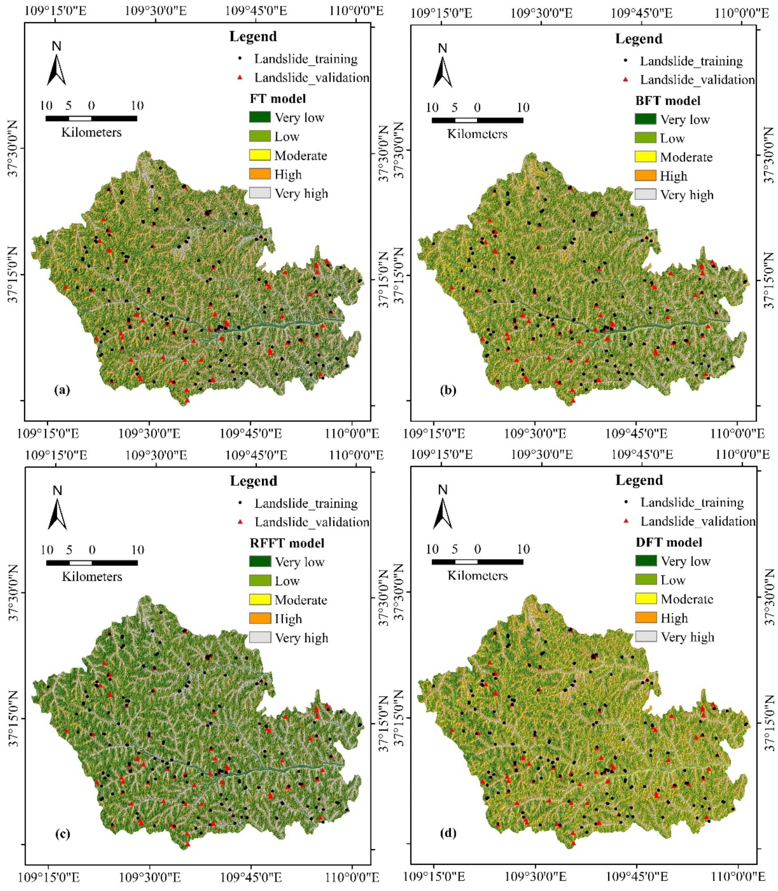
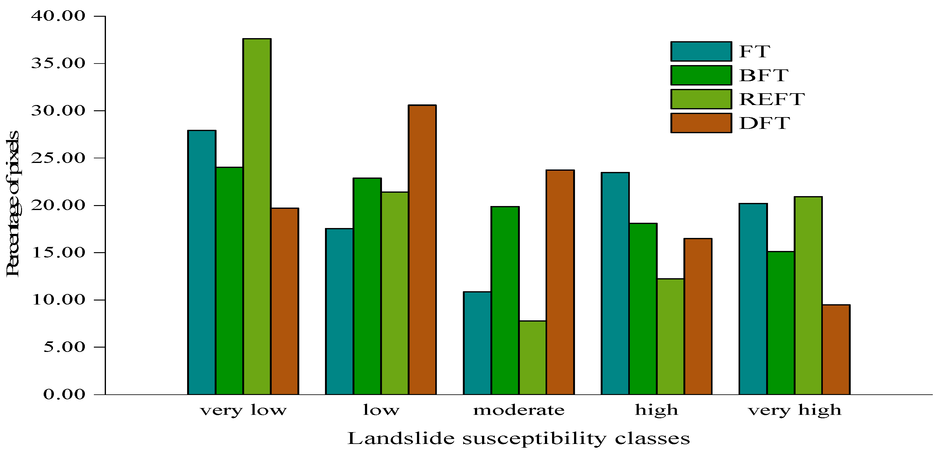
Four landslide susceptibility maps generated by FT, BFT, RFFT, and DFT models are shown in
Figure 3a–d respectively. The landslide susceptibility maps were reclassified into five classes, namely very low, low, moderate, high, and very high using the natural break method [
92]. The comparison of area sizes for each category of the four models is shown in
Figure 4. For the FT model, the largest area is the very low class (27.92%), followed by high class (23.47%), very high class (20.21%), low class (17.55%), and the smallest area is the moderate class (10.86%). For the BFT model, the percentages of very low, low, moderate, high, and very high classes are 24.02%, 22.87%, 19.88%, 18.10%, and 15.12%, respectively. The results of landslide susceptibility zoning using the RFFT model show that these percentages are 37.62% (very low), 21.41% (low), 7.79% (moderate), 12.25% (high), and 20.93% (very high), respectively. For the DFT model, the percentages of very low, low, moderate, high, and very high classes are 19.70%, 30.59%, 23.72%, 16.50%, and 9.49%, respectively.
4.4. Model Performances and Comparisons
In this study, the landslide susceptibility models were evaluated by using the areas under the ROC curves (AUC), standard error, 95% confidence interval, and significance level
p-value. The ROC curve can be used as a useful tool to indicate the quality of deterministic and probabilistic prediction system [
93,
94,
95]. The sensitivity (true positive rate) is shown as y-axis and 1-specificity (false positive rate) as x-axis [
94,
96]. The AUC values are in the range of 0.5 to 1 [
97], and the excellent attributes of the model increase with the AUC values [
98].
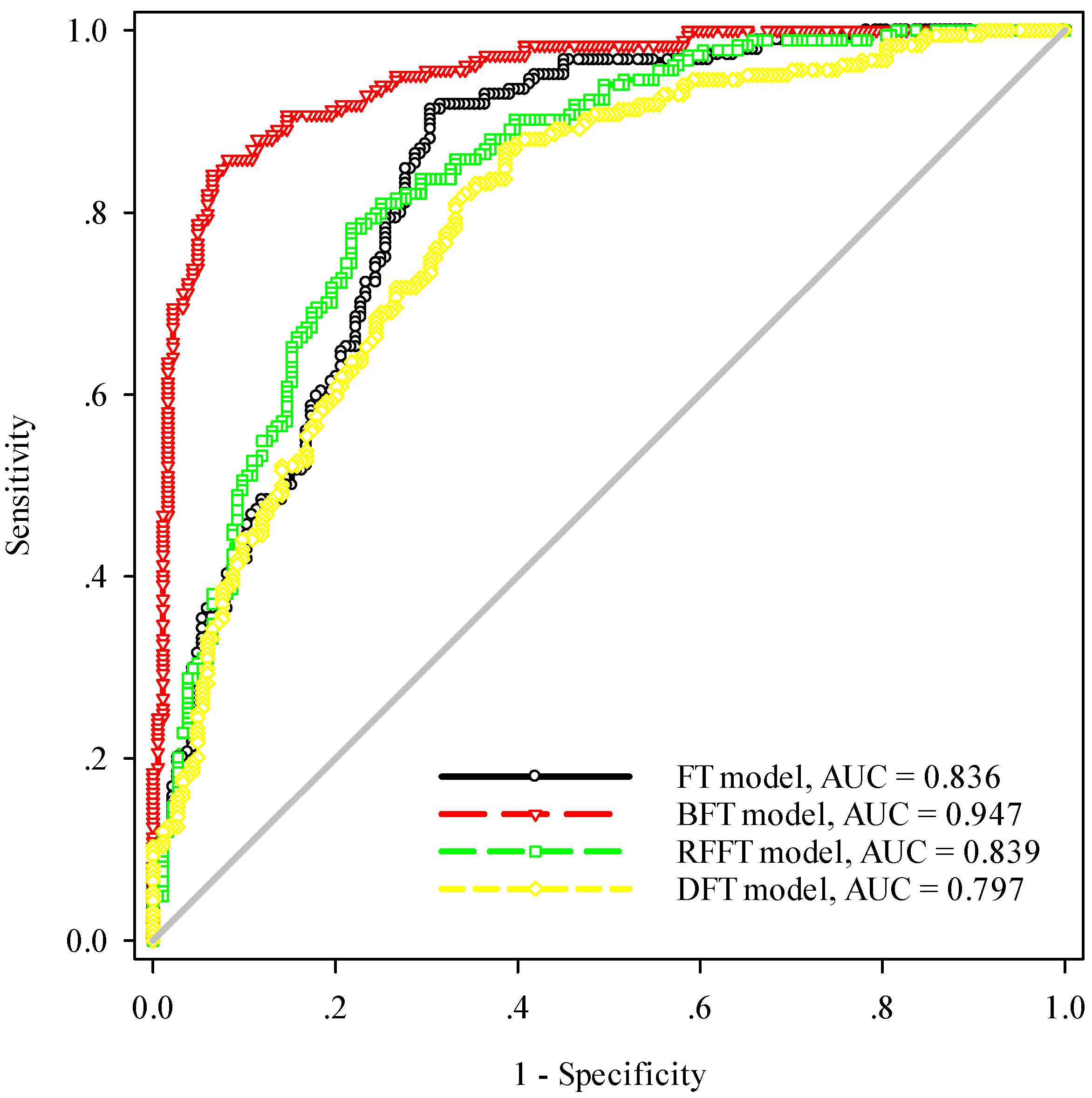
Using the training dataset, the performance of the landslide susceptibility models was evaluated (
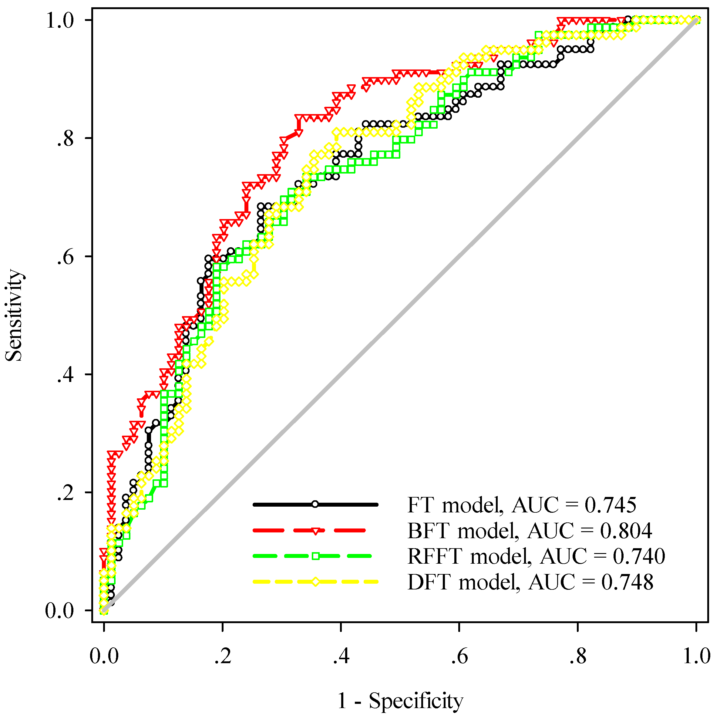
Table 4). The BFT model has the highest AUC value (0.947), the lowest standard error (0.011), and the narrowest 95% confidence interval (0.925–0.969). It is followed by the RFFT model, the FT model, and the DFT model. For the validation data, the calculation results are shown in
Table 5. The BFT model has the highest AUC value (0.804), the lowest standard error (0.035), and the narrowest 95% confidence interval (0.736–0.871). It comes before the DFT model, the FT model, and the RFFT model. These results show that all performance in the validation dataset is slightly worse than those of the training data. These results show that the BFT model is the best model among the four models, and the ensemble model is not necessarily superior to the single model.
A Chi-squared test was used to analyze the significance of the four models (
Table 6). It can be seen that only the comparison of FT and RFFT exhibits lower Chi-squared value (0.044) and higher
p-value (0.834), which indicate no significant difference between the two models. The other five groups all present larger Chi-squared values and lower
p-values. The significant differences between the models indicate that the differences between the models are good, which is more conducive to the modeling work and enables this study to obtain the susceptibility results smoothly.
5. Discussions
In this current study, the correlation analysis between conditioning factors and landslides was carried out by the CF method. The probability of landslide occurrence is in inverse correlation with elevation. This may be related to local rainfall and loess and may be related to human engineering activities. With the increase of slope angle, the degree of certainty of landslide occurrence decreases. This may be due to the larger slope angle, the less loose material or more weatherproof material. At the same time, it can be observed that most landslides occur on slopes facing south and southwest with the highest probability. This is mainly because more rain and sunshine are available to the south and landslides are prone to occur. The curvature of plan and profile shows anomalous results. The curvature of the plan (near zero) and convex plan (positive value) are highly sensitive. This anomaly may be related to the overweight effect [
28,
99,
100]. In terms of land use, the probability of landslides in residential areas is the largest, which can explain the impact of human engineering activities on landslides. For the lithology, the second group (Tertiary (T): mudstone, conglomerate) and the fourth group (Triassic (T): mudstone, sandstone, songlomerate) are more sensitive to landslide occurrence. There is groundwater flow in the relatively fractured saturated sandstone and fractured conglomerates, resulting in additional load on the mudstone, resulting in landslides [
28,
101]. The linear characteristics of the road and river buffers are inversely correlated with landslide susceptibility in the distance. Such an important result has been repeated in many kinds of literature [
6,
102,
103,
104]. However, the remaining five variables make little contributions to the occurrence of landslides.
According to ROC curve analysis (
Figure 5 and
Figure 6) and statistical index analysis (
Table 4 and
Table 5), it can be concluded that the four machine learning methods selected in the training and testing data assemble a very small
p-value and significant high performance in the 95% confidence interval. The BFT model has the highest AUC value (0.947), the lowest standard deviation (0.011), 95% confidence interval (0.925–0.969), and
p-value (<0.0001). However, the DFT model has the worst results in this study area. The DFT model has the lowest AUC value (0.797), the highest standard deviation (0.023), 95% confidence interval (0.752–0.842), and
p-value (<0.0001). There is no doubt that most ensemble models are superior to single models. However, there is still a phenomenon that the performance of hybrid machine learning methods is not always better than a single model. In order to find more optimal solutions, much more different set models should be applied to the research field.
According to the paired comparison of the performance of the models (
Table 6), the Chi-squared test shows that the Chi-squared values are relatively large. Among them, the Chi-squared value of the FT and RFFT models is smaller, the
p-value is larger, and the difference between these two models is not significant. The good results obtained from the other three groups can serve as a powerful basis for modeling in this study. At the same time, the BFT model is compared with the other three models in pairs, and the difference is significant. According to the evaluation results of various evaluation criteria, the performance of the BFT model is better than that of the RFFT model, FT model, and DFT model. As a final recommendation, the obtained results can be useful for policy planning and decision-making in areas prone to landslides. The proposed BFT model, based on performance and prediction accuracy, is suggested in the study area and other regions over the world where they have similar geo-environmental conditions with a logical caution.
6. Conclusions
This study applied functional tree-based ensemble techniques (FT model, BFT model, RFFT model, DFT model) for landslide susceptibility spatial modeling in Zichang County, China. Fourteen conditioning factors and the occurrence of landslides were used to analyze the correlation. Meanwhile, the ROC curve and statistical parameters were used to evaluate and compare the accuracy of the model results. The results showed that the prediction rate of the BFT model is the highest. Therefore, the BFT model is the best optimization ensemble model in this study, and it can be used as an advantageous and promising method for landslide susceptibility modeling. Finally, the landslide susceptibility map generated by this study can be used as an effective tool for future land planning and monitoring by government officials or research experts and scholars.


