2.1. Wastewater Treatment Plant Typical Processes
The representative processes that usually take place inside a wastewater treatment plant (WWTP) are summarized in
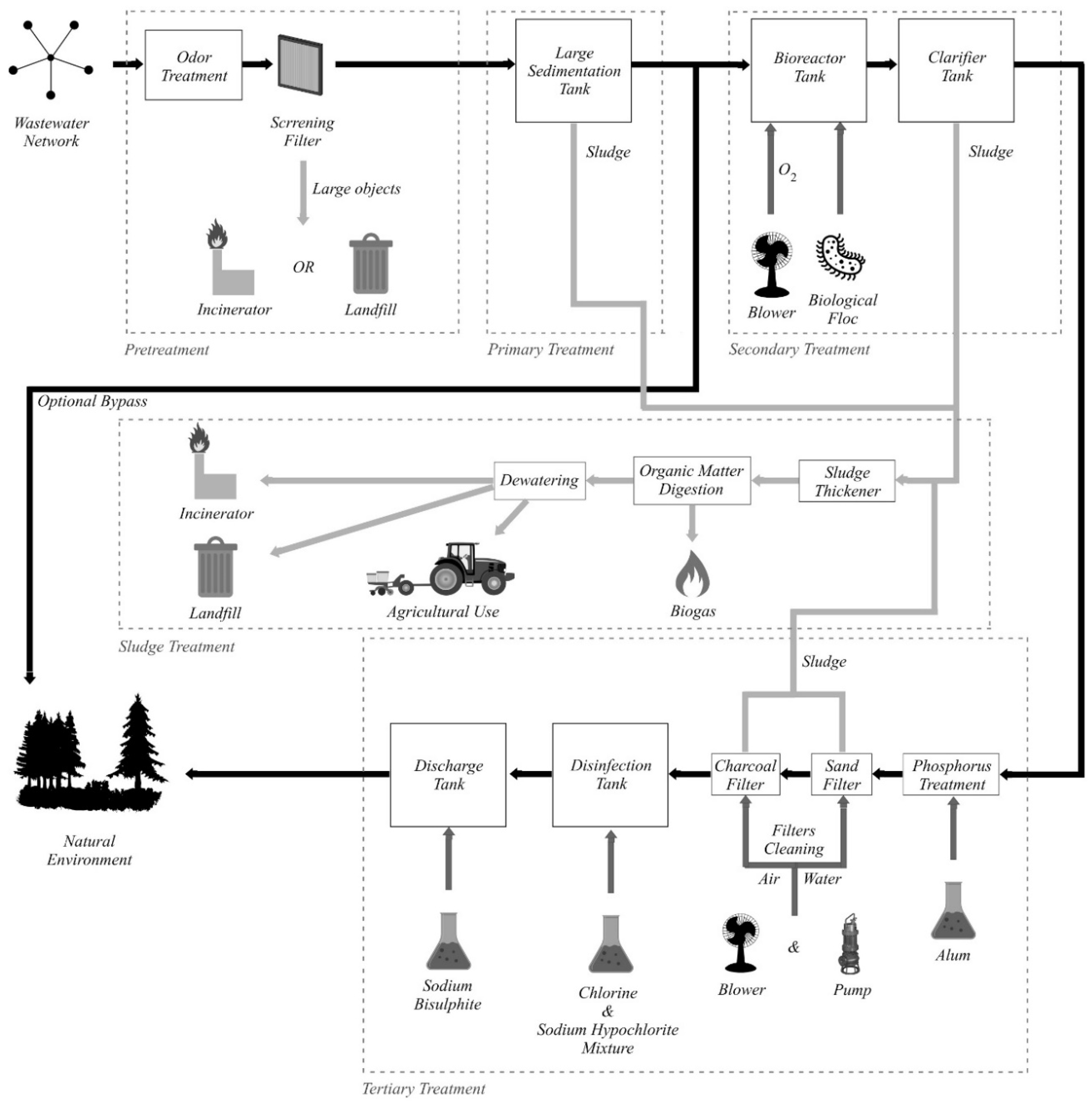
Figure 1, and further detailed in this section. The treatment process is divided, from a logical standpoint, into multiple stages: Pretreatment, primary treatment, secondary treatment, tertiary treatment, and sludge treatment.
The wastewater enters the treatment plant from the wastewater network, where the source of the water is residential, institutional, commercial, industrial, rain, or a mix of the aforementioned. After the water enters the treatment plant, the pretreatment processes are initiated. Firstly, odor treatment can be applied so that the plant surrounding areas are protected from the foul smell that naturally accompanies wastewater. The odor treatment process may not be necessary at some plants. There are two distinct methods of odor treatment: Air treatment and liquid treatment. If the air treatment method is applied, the wastewater is contained in large tanks, which are hermetically covered with specially designed odor control covers. The air trapped under the cover, inside the tanks, is extracted by a ventilation system and undergoes treatment before it is released to the environment. Regarding the liquid treatment method, different chemicals that neutralize the foul smell-producing elements are introduced in the wastewater. The second process that takes place during pretreatment is screening, where the wastewater is passed through filters in order to remove both grit and large objects such as bottles, plastics, tree branches, sanitary items, and cotton buds. It is very important to remove such objects early in the process because they can damage the plant equipment if present in future steps of the treatment process. The removed objects are either incinerated or disposed in landfills.
After the pretreatment is completed, the wastewater enters the primary treatment stage, where the remaining solid matter is separated from the wastewater. In this stage, large sedimentation tanks are used, in which the wastewater clarifies. The sludge settles at the bottom of the tank, while grease and oil rise to the surface. The sludge is removed and directed to the sludge treatment process, while the grease and oil can be used for soap making.
After the primary treatment, an optional bypass exists so that the treated water can be sent directly to the natural environment without entering the secondary and tertiary treatment stages. This bypass is used during heavy rainfall by plants that receive wastewater from a combined sewer system. In this case, the secondary and tertiary treatment stages are bypassed in order to protect them from hydraulic overloading, the mixture of sewage and rainwater receiving only primary treatment before being sent back to the natural environment. In some plants, the bypass is implemented directly at the inlet, so the wastewater is not even screened. In addition, for larger plants without a complete gravitational bypass, high-energy consumer pumps are used to transfer the untreated water directly into the emissary when the large amounts of wastewater exceed the capacity of the plant.
The secondary treatment stage objective is to remove the biological matter from the wastewater, by using a bioreactor tank where both oxygen (introduced with blowers) and a biological floc (bacteria and microorganisms that consume the remaining organic matter) are inserted into the wastewater. Before exiting the secondary treatment, wastewater is sent into a clarifier tank, where large particles settle down at the bottom (sludge) and are extracted for the sludge treatment process. In order to maintain the optimal process parameters during the biological treatment, a pH adjustment must take place, involving different chemicals (Ca(OH)2, CaCO3, Na2CO3, NaOH, etc.).
The last stage is the tertiary treatment, which is similar to the drinking water treatment process, the resulting water quality being close to drinking water quality. Firstly, a chemical compound (usually alum, Al2(SO4)3, but polyaluminum chloride or ferric chloride, FeCl3, can also be used) is injected into the wastewater in order to remove the phosphorus. In some plants, the phosphorus removal can be implemented during different stages, such as the large sedimentation tank, during biological treatment, or later, in the clarifier tank. If the phosphorus is removed by the biological treatment, the chemical treatment becomes an auxiliary method. Then, the water passes through a sand filter and a charcoal filter before entering a disinfection tank, where a mixture of chlorine and sodium hypochlorite is added. Lastly, the water is sent into the discharge tank where sodium bisulfite is used in order to chemically dechlorinate the water because residual chlorine is toxic to aquatic species. The water exiting the tertiary treatment is released into the natural environment in rivers, lakes, or other local waterways. Another important periodic process that takes place during tertiary treatment is the filters cleaning, in which the sand and charcoal filters are washed with air and water, the resulting sludge being sent to the sludge treatment process.
Each of the primary, secondary, and tertiary treatment stages produce sludge, which is also processed inside the WWTP, during the sludge treatment process. Firstly, the sludge enters the thickening procedure, which is conducted inside a sludge thickener, an equipment resembling a clarifier tank with an added stirring mechanism. Then, the sludge goes through the organic matter digestion process, which reduces the amount of organic matter in the sludge. Three different digestion options can be used: Aerobic digestion, anaerobic digestion, and composting. The digestion process can produce biogas (a mixture of CO2 and methane), which can be used at the plant for powering equipment. The last sludge treatment process is dewatering, in which the sludge is commonly placed in drying beds. The dried sludge is either burned in incinerators, sent to landfills or used as fertilizer in agriculture.
2.2. Wastewater Treatment Plant Defining Problems and Weather Dependency
Some of the defining problems that can be identified in a WWTP are:
Overloading of the plant: This can cause overheating of the blowers, which, in turn, causes a low-oxygen level in the bioreactor tank, thus reducing the efficiency of the secondary treatment stage. Plant overloading can also lead to sludge leakage from the settling tank.
High substances consumption: For instance, the odor treatment process requires continuous adjustment of the used substances, depending on the input wastewater concentration and content. The wastewater content is highly dependent on the weather conditions.
High energy costs: Around 30% of the annual WWTP operation costs is represented by the electricity consumption. Considering a developed country, an estimate of about 2–3% of the entire nation’s electrical power is consumed for wastewater treatment. This can be significantly improved by optimizing the biological treatment processes.
Equipment and/or algorithmic faults that can lead to various problems.
Undersized treatment plants: Most plants were developed 10–20 years ago, becoming undersized for the current loads since then, leading to the choice of increasing the load and costs in order to maintain a thorough cleaning process or discharging the partially treated wastewater to the environment and keeping the costs lower.
A WWTP’s operation is influenced by the weather conditions, the most significant being the precipitation amount. In case of very heavy rainfall, the WWTP may use the bypass channel, thus resulting in a high increase in operational costs (electricity and substances usage) or pollution. Even if the rain amount does not produce wastewater that can be legally sent to the environment after just primary treatment, the amount of rain highly influences the content and concentration of the wastewater present in the WWTP, which, in turn, influences the biological treatment that is applied in the secondary treatment stage and the chemical addition amounts and concentrations in the tertiary treatment. Besides rain, the temperature can also influence the WWTP, primarily from the odor treatment process standpoint, but also from the biological treatment in the secondary stage and sludge dewatering (when outdoor drying beds are used) processes standpoints. In addition, a storm or strong winds, particularly in the autumn, can generate large quantities of tree branches and leaves that can clog the screening filter during pretreatment.
Considering the typical processes that take place inside a WWTP, the defining problems and the usual weather influence on WWTPs that were previously presented, the conclusion emerges that a WWTP represents the perfect environment that can benefit from a solution capable of identifying the exact dependencies and relations that exist between the measured characteristics of a WWTP and meteorological characteristics. Furthermore, using those relations and dependencies for predicting the future evolution of the plant characteristics can provide a valuable foundation for optimizing the WWTP in order to reduce costs, lower energy consumption, decrease substance consumption, and improve maintenance. Due to these considerations, although the implemented solution presented in the following section represents a generic approach, it was deployed for testing and validating purposes in a WWTP environment, where the potential to make an impact is considerable.
2.3. The Implemented Solution
As previously mentioned, the solution that was implemented in this paper is based on the state of the research that was achieved in [
26], making use of the already-implemented both Historian application and the first level of the proactive Historian reference architecture. This already-available technological state was tested and validated in the water industry as well (results from the already-implemented first-level algorithms were used in [
27] to successfully achieve energy consumption reduction in a drinking water treatment plant, by 9% for short-term tests and by 30% for long-term tests using only part of the proposed algorithm), so it represents a reliable platform on which to build and develop, following the ultimate goal of accomplishing a fully functional proactive Historian application.
In order to merge the implementation of the second level of the reference architecture into the constantly developing application, several improvements and changes were required to the solution already implemented in [
26].
First, after long-term tests, a small improvement was made to the first-level algorithm accuracy, which, in some cases, resulted in impacting differences. The computations were adjusted in order to achieve more accuracy (in the form of decimals) in relating identified data dependencies.
Another change was made regarding the choice of the reference tag. In [
26], the implemented algorithm required the user to choose a reference from the available tags, and the remaining tags were analyzed regarding the chosen tag. In order to materialize a broader understanding of all the relations and dependencies that exist inside the monitored system, the implementation presented in this paper removed the need for choosing a reference tag. Instead of this approach, each of the monitored tags are set as a reference, one at a time, and the relations identifying algorithm developed in [
26] is run once for each reference.
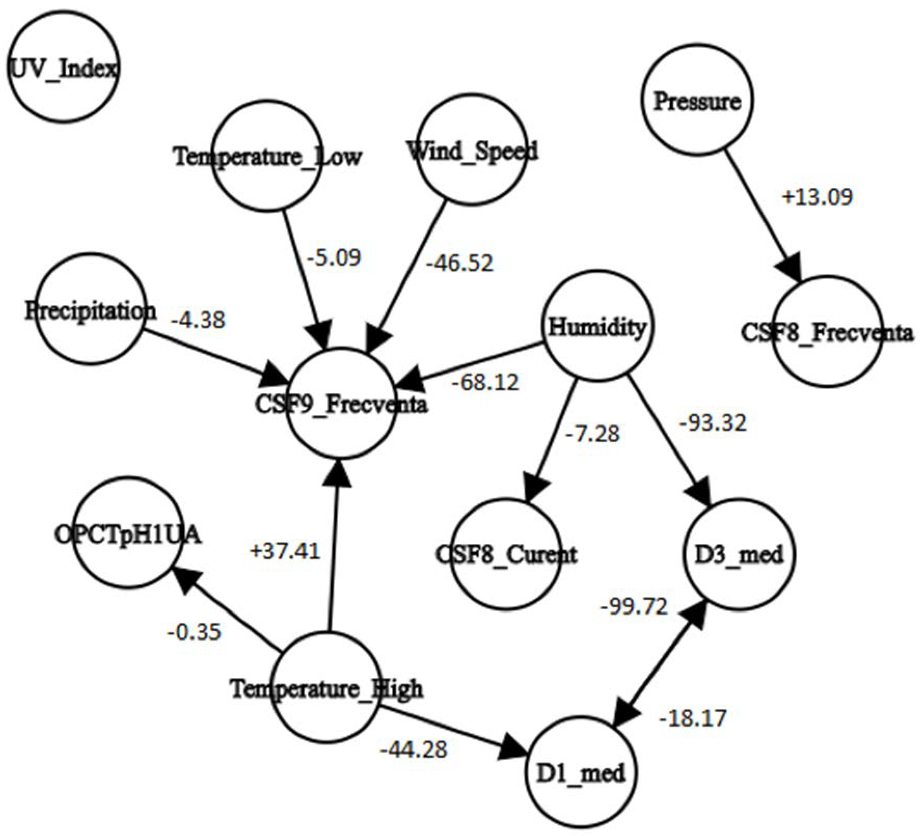
By adopting the aforementioned change related to the reference choice, new data structures are required for storing the results generated by the first-level algorithm. The relations identifying algorithm was adjusted in order to build an oriented graph of dependencies, where the results of the algorithm execution are stored. The built graph is oriented, weighted, and can contain cycles. The results are modeled using the following convention:
An arc from node i to node j with weight -N signifies when node i was set as the reference,
A dependency of node j on node i was identified,
The measured values of node j evolving inversely proportional (minus sign) to the node i values, in a quantitative proportion of N% (this percent represents the quantitative result identified by the analysis; more details regarding this percent is available in [
26]).
In the current implementation, the dependencies graph is stored using the adjacency matrix. Inside the matrix, line i contains the dependency values (please refer to [
26] for details) of all nodes j on the columns when node i is used as a reference. The dependencies graph represents essential input for the second level of the reference architecture.
The last improvement that was brought to the solution developed in [
26] consists of the possibility to involve the meteorological characteristics in the relations analysis. Historical weather data can be used in the relations and dependencies identification algorithm (at the first level of the reference architecture) at user demand. The historical weather data source is the DarkSky online service [
28]. If the user chooses to use historical weather data, the values of the relevant weather characteristics for the water industry (maximum temperature, minimum temperature, precipitation amount, humidity, atmospheric pressure, wind speed, and ultraviolet (UV) index) are obtained from [
28] for each of the days in which tags values that are involved in the analysis exist. As a requirement for obtaining the weather data, the geographical location of the monitored technical system must be provided by the user. The longitude and latitude of the location that are required for calling the weather application programming interface (API) are obtained from the user-provided address, using [
29]. After having at disposal the values of each of the 7 meteorological characteristics considered of interest, each of them is used as a reference, one at a time, in the relations identifying algorithm, which computes only the dependency of the technical system tags on the weather features. The weather features dependency on the technical system tags does not make sense, so it is not computed. As a consequence, if the user chooses to include historical weather data into the first-level algorithm analysis, the adjacency matrix of the dependencies graph will be deformed, containing i + o lines and i columns (where i signifies the number of tags from inside the monitored system and o signifies the number of tags from outside the system, essentially the number of meteorological features), meaning that the graph will not contain any arcs from a technical system-monitored tag to a weather feature.
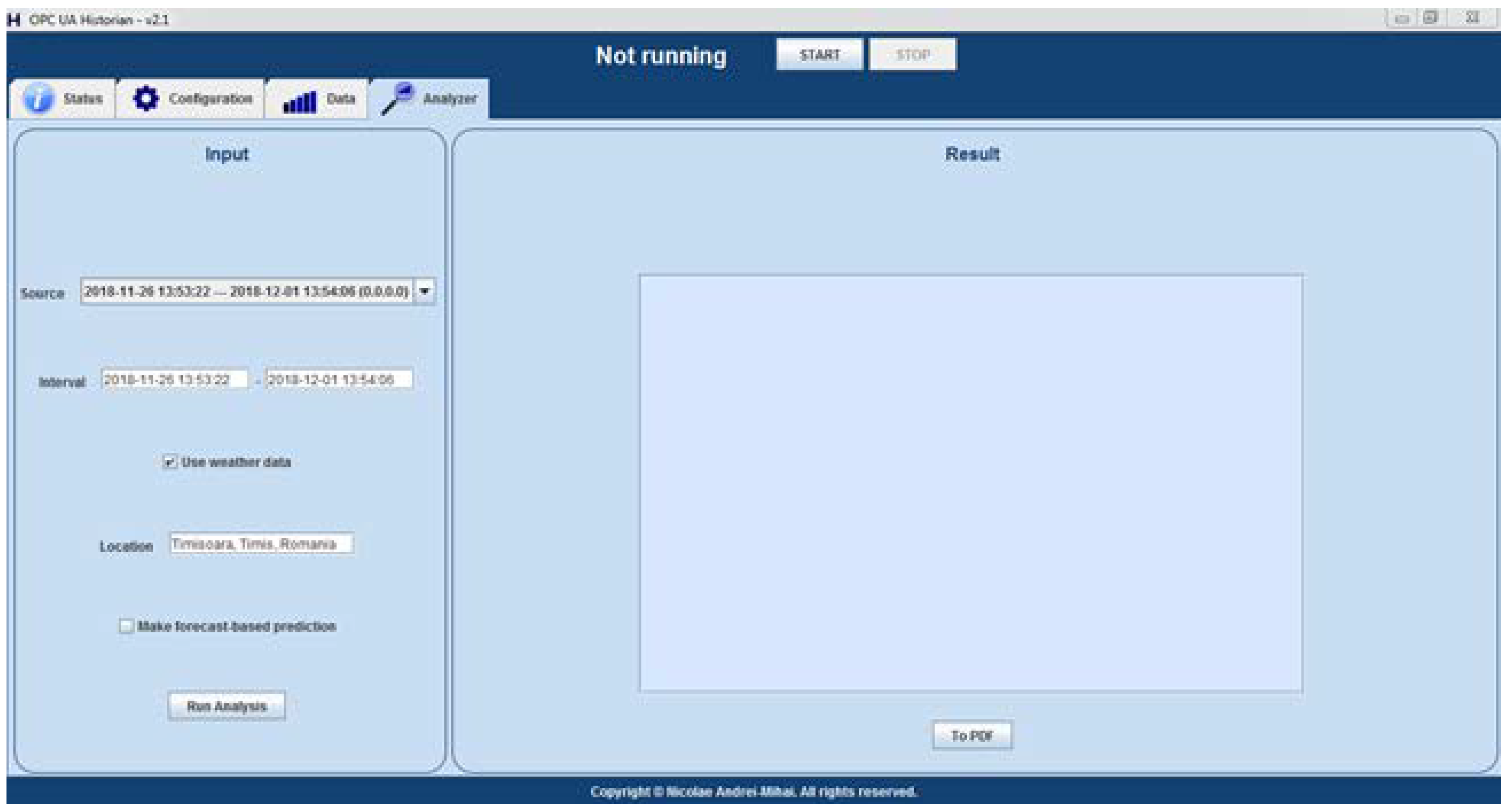
The improvements described above have led to the modification of the Historian application graphical user interface (GUI), where the new interface elements are presented in
Figure 2. The user may enable the Historian to be augmented with the predictive algorithm from the second layer of the reference architecture. This action is only allowed if the historical weather data are used in the relations and dependencies identification algorithm, at the first level.
Improvements in the developed solution from [
26] were necessary for the second level of the reference architecture. The section follows with the predictive algorithm development, placed at the second level in the reference architecture. The algorithm predicts the future evolution of the monitored technical system, based on the weather forecast and the relations and dependencies identified by the first-level algorithms.
The execution of the developed prediction algorithm is conditioned by the following prerequisites:
the dependencies graph generated by the first-level algorithms must be available;
weather forecast data must be obtained from [
28];
the most recent values of the monitored tags (which are used as initial values in the prediction process) must be extracted from the database (it is not necessary that they represent the current values; if the current values are not available, then the most recent ones are used);
Considering the valid prerequisites, the prediction algorithm is launched in execution, and
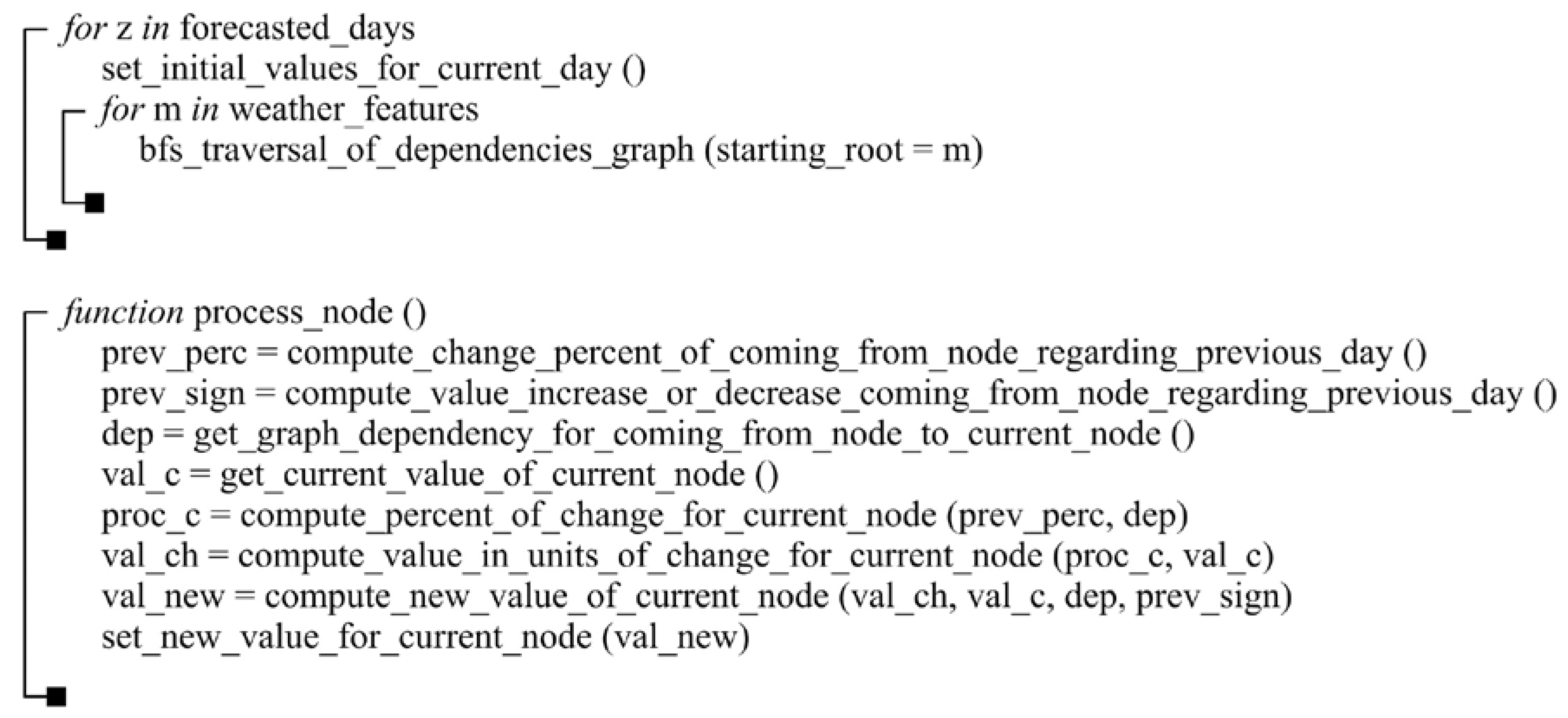
Figure 3 below summarizes an overview of the implemented algorithm.
When the predictive algorithm starts predicting values for a new day, it first initializes the monitored tag values from the technical system. For the first day of prediction, the initial values for the system tags are the most recent values from the database. For the remaining predicted days, the initial values are the same as those computed/predicted by the algorithm for the previous day.
The forecast weather data can be obtained from [
28] for a maximum of 7 days (d) ahead, thus leading to a breadth-first traversal of the dependencies graph for each of the chosen weather features in each of the 7 d ahead. The standard breadth-first traversal algorithm was adjusted in order to remember the node from which the traversal arrived at the current node, information required by the function that processes the current node (
process_node function is presented in
Figure 3). The root node of the breadth-first traversals is always a weather feature, meaning that, starting from the weather features-predicted evolution, the algorithm can predict the evolution of the technical system tags, based on the identified dependency between the weather features and the system characteristics that were identified by the first-level algorithm. By executing the breadth-first traversal, all the existing relations between the technical system tags are considered in a global manner. For instance, if technical system characteristic A is directly influenced by temperature and technical system characteristic B is inversely influenced by A, the weather forecast indicating an increase in temperature for the following day, only computing characteristic A’s new value based on the temperature increase, does not offer an accurate prediction of the system’s overall evolution, because the increase in A causes a decrease in B as well. These kinds of cases are fully covered by the implemented algorithm, thus seeking to obtain a realistic prediction.
The development of the process_node function is based on:
computing the percent of change in the previous node (the node from which the arc leading to the current node starts), by comparing the previous node’s current value and the node’s previous day value.
computing the sign of change (if the previous node’s value increased or decreased from the previous day).
using the percent of change in the previous node and the dependency from the graph, the predictive algorithm computes the percent of change for the current node (more details regarding the value of dependency in the graph can be found in [
26]).
the percent of change for the current node is further used alongside the current value of the current node in order to identify the value of change (in units) for the current node. The value of change is onwards used together with the current value of the current node, the corresponding dependency from the graph, and the sign of change for the previous node, in order to compute the new value of the current node.
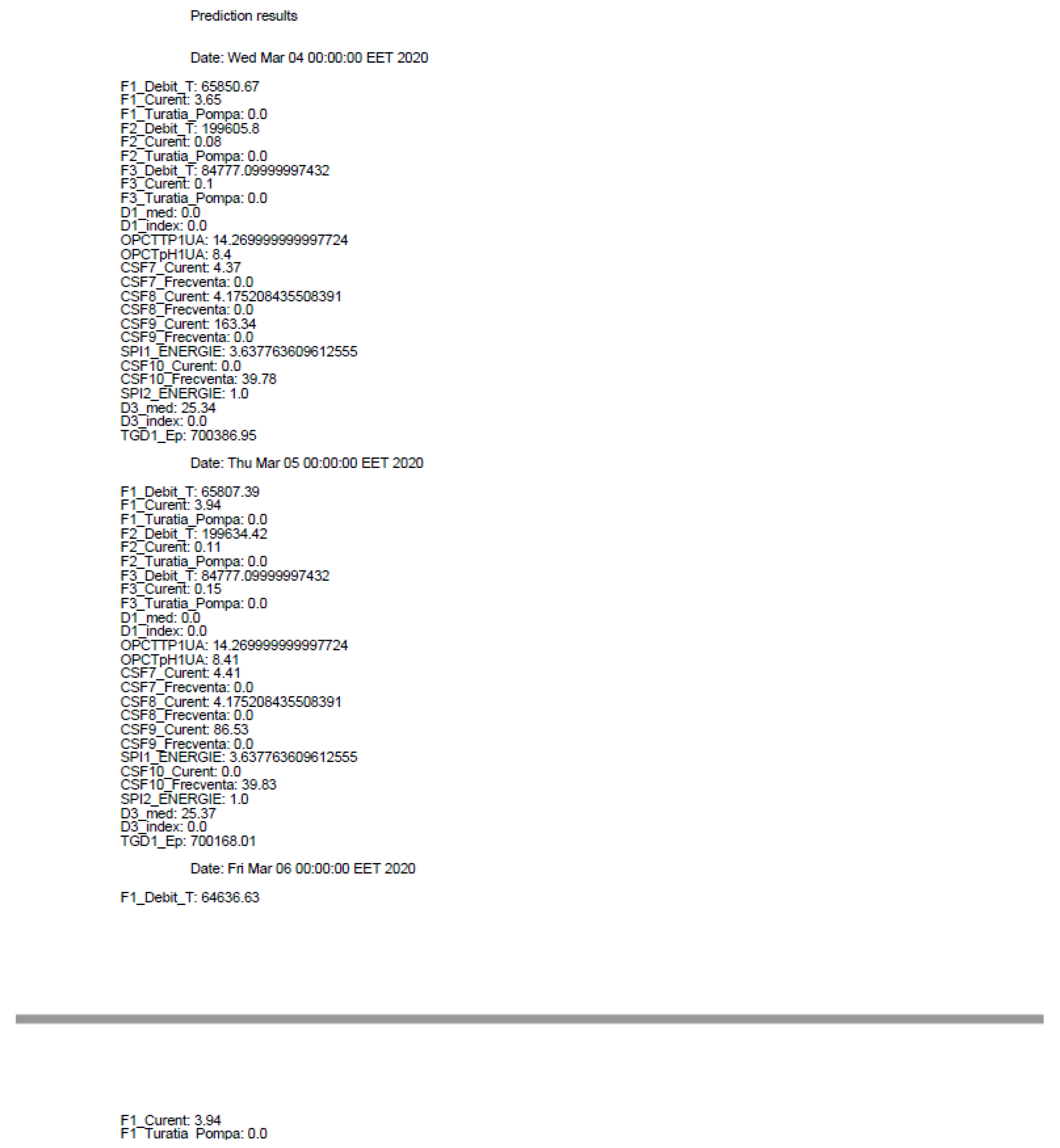
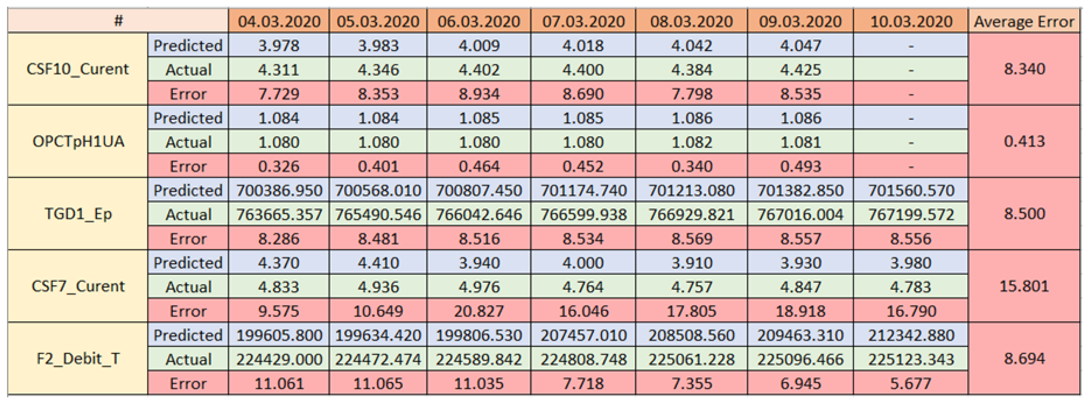
The output of the implemented algorithm represents the predicted values for the monitored tags from the technical system for 7 d of the prediction.
Thus far, the presented research implementation of the second layer follows a generic approach and can extend the water domain to any industry that relates to weather data. However, in order to apply and test the algorithm, a specific process is absolutely necessary.
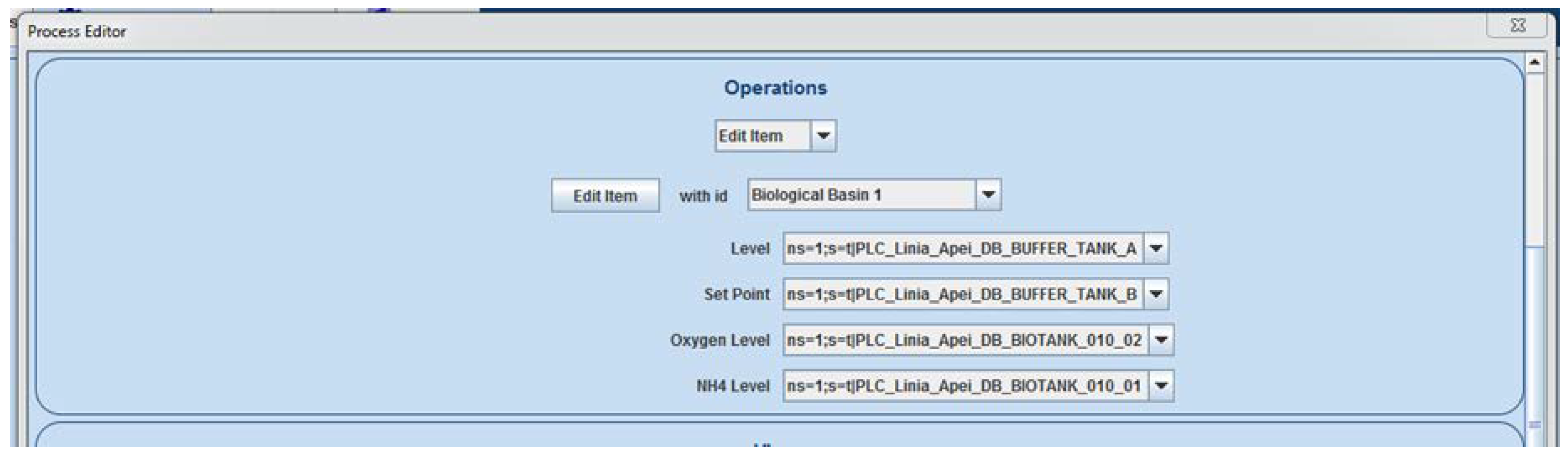
After implementing the second layer of the reference architecture, it became obvious that the relations and dependencies identification algorithm and the predictive algorithm could both receive a significant accuracy improvement by capitalizing on different process-specific information, which can be used during algorithm execution (e.g., knowing that a specific Open Platform Communications Unified Architecture (OPC UA) tag signifies the ‘fault’ code for a pump can be used during analysis in order to avoid false-positives identification for dependencies between the pump energy consumption and other values; knowing that from a process point of view, the aeration process requires a blower that implicitly consumes energy; knowing process flow of the specific process; etc.). The process-aware Historian concept is essential for correct predictions, recipes, relevant data dependency analysis, and constraint and objective function interpretation. To be able to gather and use those process-specific information, the Historian application received a newly developed software module (Process Editor), which allows the creation of a model of a monitored process, inside the Historian application. Multiple processes can be defined, from which only one can be set as the currently used one, thus facilitating an easy switch between different monitored processes. Therefore, the process-aware Historian will request essential data mapping from the user according to the predefined process components characteristics. A defined process inside the Process Editor contains steps, which, in turn, contains items. There are multiple predefined item types from which the user can choose (water source, air blower, pump, flowmeter, water tank, etc.), each item having its own predefined characteristics (example for a biological basin: Level, set point, oxygen level, NH
4 level). For each characteristic, the user can set an OPC UA tag from the server list, thus assigning a meaning to each monitored OPC UA tag.
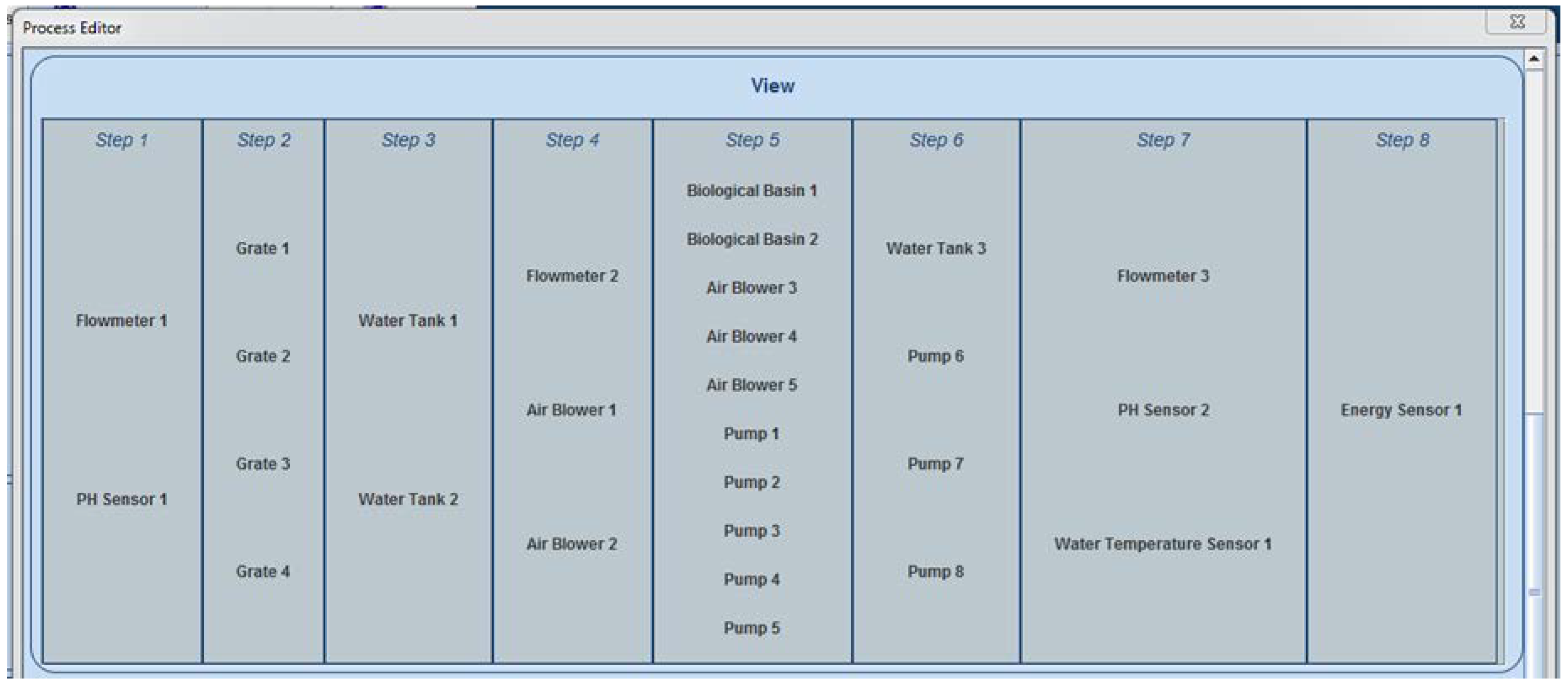
Figure 4 presents the editing of an item from the Process Editor, while
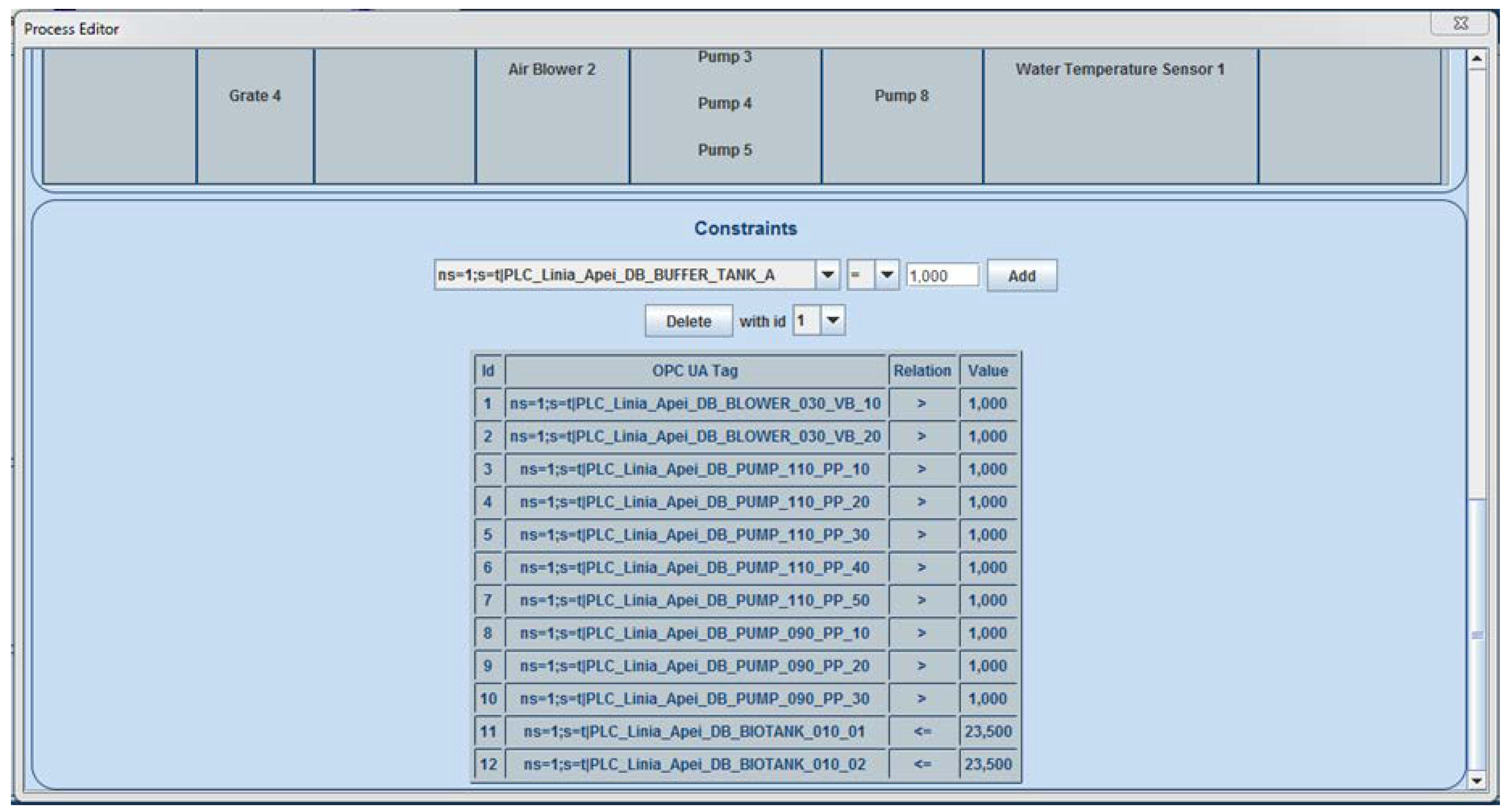
Figure 5 presents a process of a WWTP, as defined in the Historian Process Editor. Furthermore, the possibility of adding different constraints to the process was also implemented and is illustrated in
Figure 6.
Considering the generic approach of the Historian application, which is intended at not restricting it only to the water industry, even though predefined item types and characteristics are offered, the implementation created a generic framework, which makes use of two Java String arrays (containing all the predefined elements), for both building the required GUI elements and interacting with the Extensible Markup Language (XML) structure used for storing the process definition. This approach implies that adding and/or removing items or item characteristics requires just a small change in an array of Strings (no additional changes are required at GUI elements building or XML interaction), thus keeping the application suitable for easy expansion toward other industries.


