1. Introduction
Magnetoencephalography (MEG) is a technique employing sensitive sensors to detect the weak magnetic field signal generated by the neurons of the brain without invasion or damage [
1,
2,
3]. The detected data can be used to analyze the vital information of the brain. Currently, MEG is not only applied in advanced brain function research, such as auditory, vision, sensation, and even recognition [
4,
5,
6,
7,
8,
9], but is also widely used in epilepsy surgery and the diagnoses of Parkinson’s disease, psychosis, and other brain function diseases [
10,
11,
12,
13,
14].
Since the magnetic signal emitted from brain activities is feeble, the magnetic shielding room (MSR) is needed during the MEG recordings. In addition, other methods are also applied to stabilize the magnetic field with different types of sensors [
15,
16,
17,
18,
19,
20]. Nevertheless, if the original detected signal is directly observed, little information can be obtained owing to the existence of various types of noise [
2,
21]. Among all kinds of noise, the biological signals, such as blinks, eye movements, and heartbeats, are unique and the most disturbing for the MEG [
22]. Interferences caused by these biological signals are called artifacts, among which the blink artifacts are the most significant and must be removed. In order to remove blink artifacts and observe the weak signal triggered by the brain activities more precisely [
23,
24], the original data need to be processed. Signal space projection (SSP) [
25,
26,
27,
28] and independent component analysis (ICA) [
29,
30] are widely used to remove the blinks and other artifacts in the MEG. However, these two methods may need extra electrodes to measure the blink signals in the electrooculogram (EOG) and decide the occurrence time of the blink artifacts in the MEG for practical use. A professional staff is also needed to identify the blink artifacts. To make up for the shortcomings of these two algorithms, some decent automatic processes for artifacts rejection based on statistics have been proposed by many research groups [
31,
32,
33,
34,
35]. Machine learning algorithms are also introduced into the MEG data processing [
36,
37].
Some algorithms [
38,
39] have been proposed to classify different artifacts in the MEG and EEG (electroencephalography) based on machine learning. Most of these algorithms require data preprocessing, such as ICA, to extract the feature vectors of the artifacts. The preprocessing essentially reduces the dimension of the original detected MEG signal and then recombines these signals. The dimension reduction distorts the spatial dimension of the detected signal, which not only results in the loss of information of the original signal, but also adds some redundant messages into the MEG signal segments that are not influenced by the blink artifacts. In this work, we use the artificial neural network (ANN) to analyze the blink artifacts from the original detected MEG signal, and make full use of the information of their spatial distribution features, so as to realize its automatic identification.
With the development of computer science and information theory, the ANN is proposed as a powerful computing tool [
40,
41,
42]. The ANN is a model built from the human brain neural network and can form different structures according to different connection methods, aiming to solve classification problems. It is a persuasive tool to extract data characteristics and eliminate noise, which plays a major role in various fields, such as automatic speech recognition (ASR) [
43,
44], computer image processing [
45], and biomedical imaging [
46,
47].
The objective of the present study is to identify blink artifacts from the original detected MEG data. To address the aim, the original detected MEG data are color-coded into 2D images to display the spatial distribution of the blink artifacts, which are characteristic. These 2D images are taken as the input of the GoogLeNet [
48] to automatically identify the blink artifacts. GoogLeNet is a convolutional neural network (CNN), which is a typical ANN and can recognize image features, indicating that no extra electrodes and professional confirmation are needed for artifacts identification and providing a novel perspective for the analysis of artifacts in the MEG. The total solution is shown to have the potential to assist the SSP and the ICA algorithm to realize the automatic and on-the-fly rejection for artifacts.
2. Materials and Methods
Data processing for the original detected MEG signal aims to remove noise, including line frequency noise, blink artifacts, eye movement artifacts, cardiac artifacts, etc. Blink artifacts are the noise that has the greatest influence on the original detected MEG signal. In order to remove the blink artifacts with the SSP and the ICA algorithm, the occurrence time of the blink artifacts should firstly be decided from the blink signals in the EOG. In this work, an ANN is utilized to recognize the spatial distribution characteristics of the blink artifacts, providing a new solution to automatically identify the blink artifacts from the original detected MEG data in real time. The process includes three sequential steps: obtaining the data, training the network, and testing the network.
2.1. Data Collection
The eight data sets used in this work come from Brainstorm website [
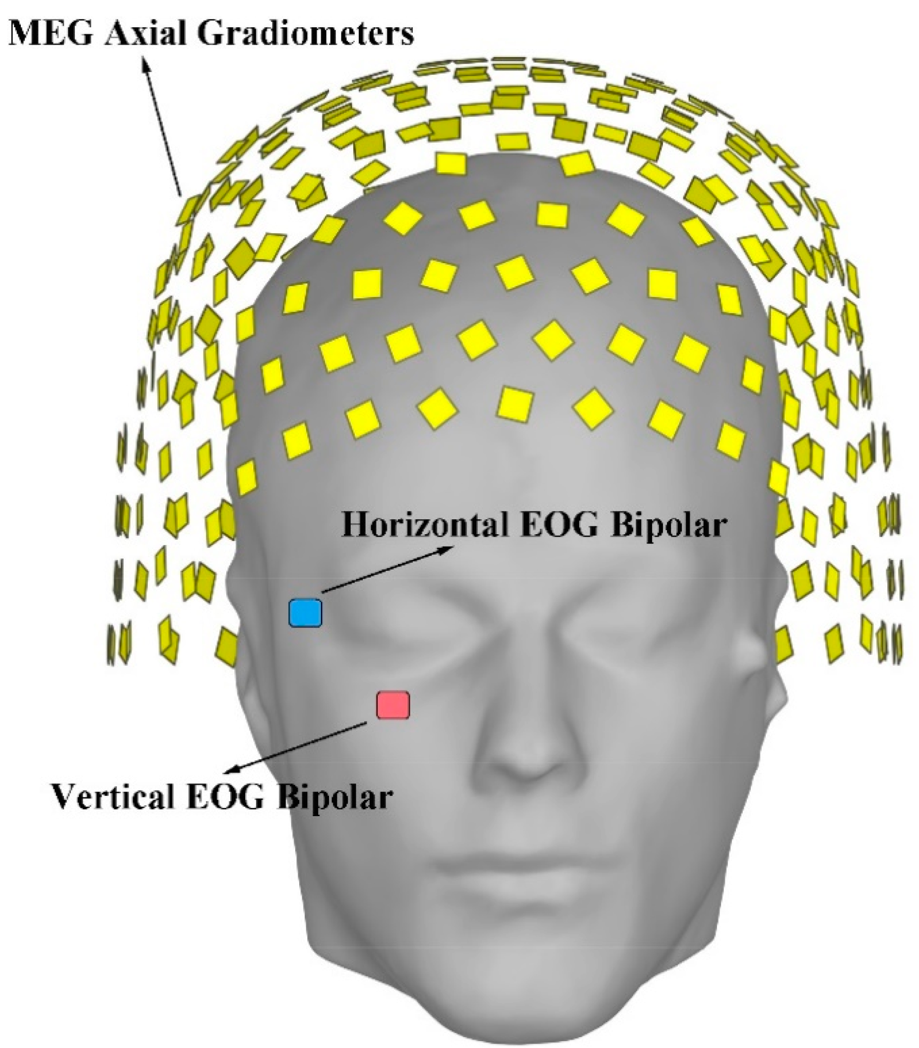
49]. Four data sets are used to train the ANN, and all data sets are used to test the trained ANN. These data are recorded with a SQUID (superconducting quantum interference device) MEG system, which includes 274 sensors. The device is produced by the CTF corporation, Canada. The distribution of its sensors is shown in
Figure 1 and the sensors involved in the data recording are given in
Table 1.
Eight MEG signal data sets are recorded by 274 magnetic field sensors. The 1st and 2nd data sets have a time duration of 360 s, the remaining six data sets have a time duration of 300 s, and all data sets have a sampling rate of 600 Hz. These data sets are collected from 4 different subjects and every two data sets are collected from the same subject, as is shown in
Table 2. In total, 701 blink artifacts are contained in these data sets. It is a large enough data set for the artificial neural network (ANN) to extract spatial distribution characteristics.
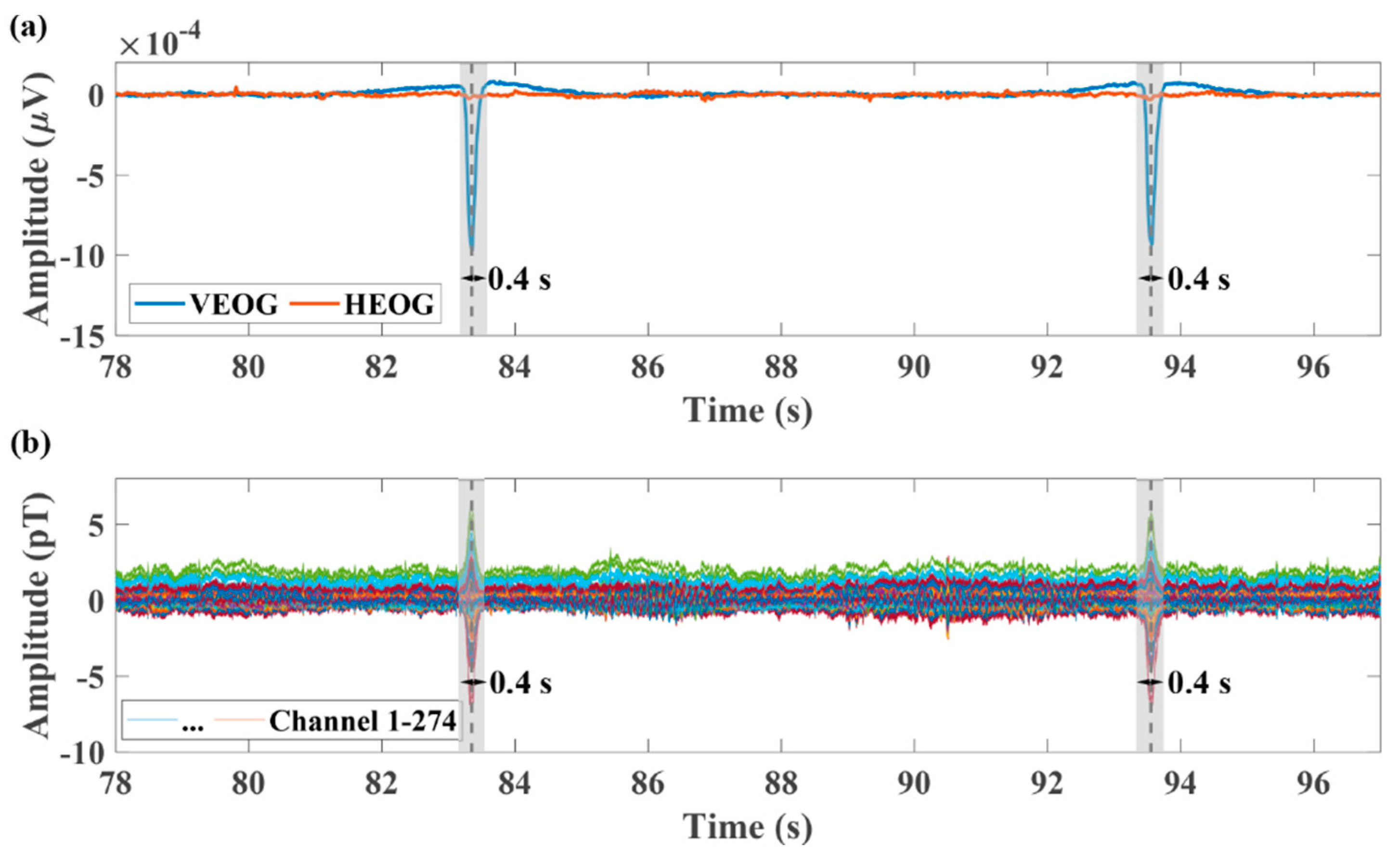
Filters are used to preprocess the original detected MEG signal data. A second-order infinite impulse response (IIR) notch filter with 3 dB bandwidth of 2 Hz is used to clear line frequency noise of 60, 120, and 180 Hz. An even-order linear phase finite impulse response (FIR) low-pass 200 Hz filter with 60 dB stopband attenuation is performed on the signal to remove other noise and leave the MEG signal. In addition, the blink signal in the EOG is employed to mark the blink artifacts in the MEG. In
Figure 2a, according to the obvious blink signals provided by the vertical eye movement signal (VEOG), we can mark the time point of the emergence of the blink artifacts in the MEG signal, as is shown in
Figure 2b. These time points allow us to accurately intercept the blink artifacts in the MEG as training data. In addition, when the ANN is used to identify the blink artifacts, we can also use these time points to compare the identification results. This step is often referred to as data calibration in machine learning. It should be noted that in Brainstorm, the blink signals in the EOG are used to determine the blink artifacts in the MEG. The specific algorithm is used to detect the rising edge of the blink signals to get its occurrence time. The detection algorithm needs to set fixed parameters including threshold, duration, frequency, etc. Nevertheless, because the blink signals are not always the same, coupled with the interference of other sources of noise, this method is not always effective. The new identification method can determine whether the sampled data are the blink artifact from the original detected MEG data. The center of all sampling time points identified as the blink artifacts is considered to be the time when each blink artifact appears, as is shown in the shadow of
Figure 2.
2.2. Training Data Set
In order to directly identify the blink artifacts from the original detected MEG data, we need to train the ANN with the calibrated MEG signal first. In this work, the GoogLeNet is utilized to recognize the spatial distribution characteristics of the blink artifacts, which are highlighted by drawing 2D images. These 2D images are our training data.
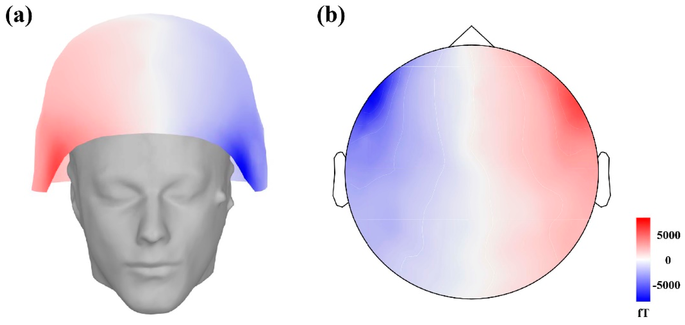
Since each sampling data point is recorded by 274 sensors located at different locations on the head surface, it comprises a matrix with dimensions of 274 × 1. Each sampling data point can be used to draw a 3D image of the signal strength at different locations on the head surface, as is shown in
Figure 3a. One second of MEG data can be used to draw 600 images. However, 3D images are difficult for the GoogLeNet to recognize. The locations of the sensors distributed on a 3D surface can be topographically mapped onto a 2D plane. The signal amplitude measured with each sensor is subsequently color-coded as 2D images, as is shown in
Figure 3b. These 2D images can be the input of the GoogLeNet. According to the calibrated MEG signal, a total of 66,780 2D images can be obtained with 8 data sets for training and testing of the ANN. The 1st, 3rd, 5th, and 7th data sets are employed to draw the training and validation 2D images. All data sets are employed to draw the testing 2D images.
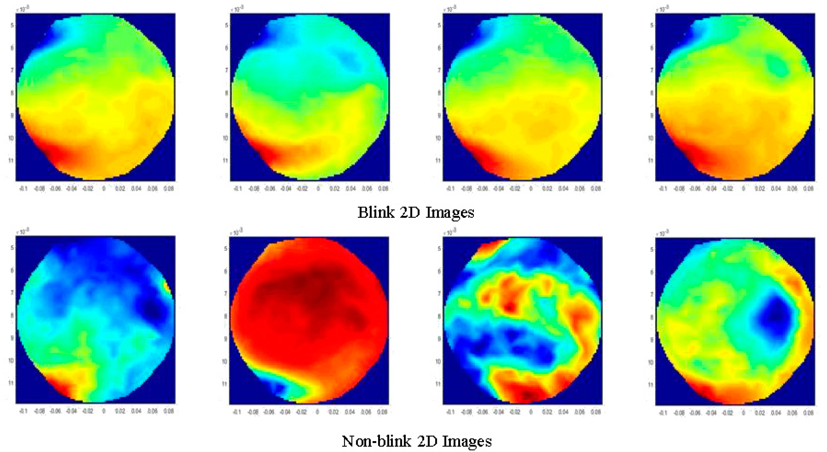
The 1st data set contains 20 blink artifacts, each of which lasts for approximately 0.4 s. In order to obtain the spatial information of the blink artifacts and expand the training data set, we capture a 0.1 s signal segment of the center of the blink artifacts and label these data as blink data, which means that we have a length of 0.1 (seconds) × 20 (blinks) × 600 (sampling rate) blink data. Since it is recorded with 274 sensors, the training data has the form of a matrix with dimensions of 274 × 1200. For signal segments with no artifacts, we randomly select 2000 sampled data for training and label them as non-blink data. Thus, we get a data matrix with dimensions of 274 × 3200, which can be used to draw 3200 2D images to train the ANN. Four 2D images of blink data and four 2D images of non-blink data are randomly selected from 3200 2D images, as is shown in
Figure 4. Similarly, the 3rd, 5th, and 7th data sets include 71, 65, and 211 blink artifacts, respectively. We can get 2820, 3900, and 12,660 blink 2D images from these 3 data sets, respectively. At the same time, 3000, 4000, and 12,000 non-blink 2D images can be randomly selected from these data sets, respectively. These 2D images are then employed to train the ANN. The training data set is shown in
Table 2.
2.3. Artificial Neural Network
After obtaining the training data, the pre-trained network GoogLeNet is adopted to recognize the blink artifacts. It is a 144-layer CNN. Each layer of the network architecture can be regarded as a filter. The initial layer is primarily used to identify common features of the image, such as blobs, edges, and colors. The subsequent layers focus on more specific features to classify categories. GoogLeNet is pre-trained to classify images into 1000 object categories. According to the experiments of EEG data processing using the ANN [
50], we need to readjust and retrain GoogLeNet for blink artifacts recognition, and specific adjustment of its 3 layers is made. We use MATLAB [
51] to carry out the data processing.
To prevent over-fitting, a dropout layer is used in the original net. The dropout layer randomly sets input elements to zero with a given probability, and the default value is 0.5. Because we have fewer categories, in order to prevent overfitting, we replace the final dropout layer in the network with a new dropout layer with the probability of 0.6. Convolutional layers of the network extract image features. These features are employed to classify the input image by the last connected layer and classification layer. These two layers of the original GoogLeNet contain information on how to combine these features into class probabilities, a loss value, and predicted labels. To classify the blink and non-blink images, we replace these two layers with new layers adapted to the data. The last connected layer is replaced by a new fully-connected layer with the number of filters equal to the number of classes (blink and non-blink). The classification layer is replaced by a new one without class labels, and it is automatically set as the output class during the network training.
Finally, we set the initial learning rate as 0.0001, the epoch as 10, and set a random seed as the default value in MATLAB [
52]. The learning rate determines the variation range of parameters in the ANN and is a decreasing function of the epoch. The epoch represents the number of times the ANN is trained with the same set of training data. We use 80% of the images in training data for training and the remainder for validation. The training data comes from the first data set, which is also adopted to evaluate the recognition efficiency. The results are described in the section Results.
2.4. Testing
All 8 data sets are used to verify the efficiency of the method for blink artifacts identification. These data sets are taken as the testing data source. During 360 s (300 s) of data collection, 60 sampling data can be obtained every 0.1 s. Only one piece of sampling data is randomly selected and made into 2D images for identification. We can obtain 3600 2D images from the 1st and 2nd data sets and 3000 2D images from the remaining 6 data sets to be the testing data, as is shown in
Table 2. The 2D image of the testing data set is then input into the trained ANN to identify whether it is a blink artifact. The identification results can be plotted in time for comparison with the MEG and the EOG signal. Detailed identification results are described in the
Supplementary Materials.
In addition, in order to evaluate the identification results, we perform statistical calculation on the final identification results. The detection accuracy of each data set is obtained. The accuracy can be calculated as follows:
False alarm represents that there are no blink artifacts in the original MEG signal data, but it is identified as blink artifacts by ANN. Missing alarm represents that the blink artifacts exist in the original MEG signal data, but they are not identified by ANN.
3. Results
In the first data set, there are practically 20 blinks [
49]. The ANN identifies 20 blinks in total, with an accuracy of 100%. For the second data set, that contains 20 blinks, the ANN identifies 23 blinks. There are three false alarms at 124.7, 149.3, and 300.6 s. Compared with the 100% accuracy for the first data set, it can be thought that the false alarms are caused by insufficient training data. On the one hand, the fact that it can identify all blinks implies that the method is effective. On the other hand, the false alarms indicate that it does not learn enough data features. The false alarms mainly result from the MEG signal which has similar characteristics to the blink artifacts. The non-blink 2D images we randomly selected may not be enough to cover all the MEG signal features, making it difficult for ANN to distinguish the MEG signals that similar to the blink artifacts. For the third and fourth data sets, that include 47 and 80 blink artifacts, there are one and five false alarms, respectively, and zero missing alarms. The fifth and sixth data sets contain 65 and 78 blink artifacts, respectively. The identification results show there are zero and three false alarms, respectively, and one missing alarm in each. At last, 211 and 180 blink artifacts are included in the seventh and eighth data sets, respectively. The ANN has 18 and 30 false detections and 4 and 11 missing detections, respectively, for these two data sets. The identification results for the eight data sets are summarized in
Table 3.
In addition, test accuracies of the first, third, fifth, and seventh data sets tend to be 100%, because the testing data from these data sets are similar to the training data set. For the other four data sets, we get accuracies of 86.96%, 94.12%, 95.06%, and 80.48% for the second, fourth, sixth, and eighth data sets, respectively. The eighth data set has distinctly worse results than other data sets, because the eighth MEG signal data set, measured from the fourth subject, contains more environmental noise (please see
Supplementary Materials for more details). Since we only filter the original MEG signal data, different measurement environments will have a great impact on the identification results.
4. Discussion
In this work, blink artifacts identification is achieved by the ANN. Eight data sets collected from four different subjects are used to verify the recognition effect of the ANN. The first, third, fifth, and seventh data sets are employed to train the ANN. All eight data sets are used to test the ANN. The accuracy of the identification results shows the method can recognize the blink artifacts in the MEG signal. Nevertheless, the false alarms and the missing alarms appear. The missing alarms mainly result from insufficient training data. The MEG signals are signals with high inter-individual variability. Different subjects may produce different MEG signals. If we used the MEG data from one subject to train the network, and then used the trained network to identify the blink artifacts measured from another subject, the accuracy would drop dramatically. Considering that, using the ANN to recognize the blink artifacts generated by different subjects still needs further research. In addition, due to the different states of the subject during the experiment and the different measuring environment, the blink signals produced by the same subject may vary. The false alarms may be bound to the characteristics of the MEG signals and not to the characteristics of the blink artifacts. Some MEG signals may exhibit similar characteristics to the blink artifacts, resulting in misjudgment by the ANN. If various training data sets could be used to train the network, the recognition accuracy might be further improved, which needs to be proved by further experiments.
When recognizing spatial distribution characteristics of blink artifacts using the ANN, the identification algorithm does not introduce additional electrodes, and it can be implemented automatically and simultaneously with data measurement. These advantages endow the method with the ability, when combined with the SSP and the ICA algorithm, to realize the automatic and on-the-fly rejection for blink artifacts. Nevertheless, volumes of calibrated data are required to train the ANN to improve its accuracy. In this work, 66,780 2D images generated from eight MEG signal data sets are used for training and testing GoogLeNet. If we want to apply this method to practical problems, various types of artifacts are needed to train the ANN, which are missing in this experiment and need to be further supplemented.
In addition, if other artifacts data, such as eye movement artifacts and cardiac artifacts, are collected and employed for feature extraction, the ANN has the potential to classify and identify these artifacts in the MEG. The eye movement and cardiac artifacts are regarded as noise in the MEG and need to be removed, but for some other typical applications, such as the research on relationships between the eye movements and human brain activities, our method provides thoughts to extract the information from these artifacts. In addition, the machine learning algorithm has the potential to be migrated and applied to signal source estimation in the future. In magnetic source imaging (MSI), a more suitable network could be employed to classify the signals emitted from different parts of the brain, to establish the map between the location of the signal sources and the detected signal. Furthermore, the ANN should be capable of making a preliminary diagnosis by identifying the characteristics of the MSI. If such work can be realized through machine learning, it would hopefully reduce the burden of doctors and improve the efficiency of diagnosis and treatment.
5. Conclusions
In this work, a method based on the ANN for the identification of the blink artifacts is proposed, and 66,780 2D images generated from eight MEG signal data sets are used to train and test the convolutional artificial neural network, in which GoogLeNet is used as a pre-trained input. The identification based on the ANN enables us to identify the blink artifacts directly from the original detected MEG signal, rather than the EOG detected by electrodes. This method has the potential to be combined with the traditional SSP and ICA algorithm to realize the automatic rejection for blink artifacts.
The spatial distribution characteristics of blink artifacts can be recognized by ANN in this method. MEG signals with similar characteristics, such as cardiac artifacts, auditory evoked magnetic fields and visual evoked magnetic fields, can also be identified by this method in the future. In addition, ANN is expected to be used in magnetic source imaging to establish the map between the signal space and the source space. These methods are still to be explored in the future.
Author Contributions
Conceptualization, Y.F.; methodology, Y.F.; software, Y.F.; validation, Y.F., T.W., J.Z., and J.X.; formal analysis, Y.F.; investigation, Y.F.; resources, Y.F., and W.X.; data curation, Y.F.; writing—original draft preparation, Y.F.; writing—review and editing, Y.F., T.W., J.Z., and J.X.; visualization, Y.F.; supervision, Y.F., T.W., and J.Z.; project administration, T.W. and H.G.; funding acquisition, H.G. All authors have read and agreed to the published version of the manuscript.
Funding
This research was funded by the National Natural Science Foundation of China, grant numbers are 61571018, 61531003 and 91436210, and the National Key Research and Development Program.
Institutional Review Board Statement
Not applicable.
Informed Consent Statement
Not applicable.
Data Availability Statement
The eight MEG signal data sets used in this paper are obtained from the open database of Brainstorm software, and its website is:
http://neuroimage.usc.edu/brainstorm (accessed on 17 February 2021).
Acknowledgments
This project is supported by the National Natural Science Foundation of China (61571018, 61531003 and 91436210) and the National Key Research and Development Program. We are also grateful for the open data source in Brainstorm software and its website is:
http://neuroimage.usc.edu/brainstorm (accessed on 17 February 2021).
Conflicts of Interest
The authors declare no conflict of interest.
References
- Babiloni, C.; Pizzella, V.; Del Gratta, C.; Ferretti, A.; Romani, G.L. Fundamentals of Electroencefalography, Magnetoencefalography, and Functional Magnetic Resonance Imaging. Int. Rev. Neurobiol. 2009, 86, 67–80. [Google Scholar] [CrossRef] [PubMed]
- Hämäläinen, M.; Hari, R.; Ilmoniemi, R.J.; Knuutila, J.; Lounasmaa, O.V. Magnetoencephalography—Theory, instrumentation, and applications to noninvasive studies of the working human brain. Rev. Mod. Phys. 1993, 65, 413–497. [Google Scholar] [CrossRef] [Green Version]
- Hari, R.; Salmelin, R. Magnetoencephalography: From SQUIDs to neuroscience. Neuroimage 2012, 61, 386–396. [Google Scholar] [CrossRef]
- Almubarak, S.; Alexopoulos, A.; Von-Podewils, F.; Wang, Z.I.; Kakisaka, Y.; Mosher, J.C.; Bulacio, J.; Gonzalez-Martinez, J.; Bingaman, W.; Burgess, R.C. The correlation of magnetoencephalography to intracranial EEG in localizing the epileptogenic zone: A study of the surgical resection outcome. Epilepsy Res. 2014, 108, 1581–1590. [Google Scholar] [CrossRef] [PubMed]
- Wennberg, R. Magnetic source imaging versus intracranial electroencephalogram: Neocortical versus temporolimbic epilepsy surgery. Ann. Neurol. 2006, 60, 271. [Google Scholar] [CrossRef] [PubMed]
- Stefan, H.; Hummel, C.; Scheler, G.; Genow, A.; Druschky, K.; Tilz, C.; Kaltenhäuser, M.; Hopfengärtner, R.; Buchfelder, M.; Romstöck, J. Magnetic brain source imaging of focal epileptic activity: A synopsis of 455 cases. Brain 2003, 126, 2396–2405. [Google Scholar] [CrossRef] [Green Version]
- De Tiège, X.; Lundqvist, D.D.; Beniczky, S.S.; Seri, S.S.; Paetau, R.R. Current clinical magnetoencephalography practice across Europe: Are we closer to use MEG as an established clinical tool? Seizure 2017, 50, 53–59. [Google Scholar] [CrossRef] [Green Version]
- Jmail, N.; Gavaret, M.; Bartolomei, F.; Chauvel, P.; Badier, J.-M.; Bénar, C.-G. Comparison of Brain Networks During Interictal Oscillations and Spikes on Magnetoencephalography and Intracerebral EEG. Brain Topogr. 2016, 29, 752–765. [Google Scholar] [CrossRef] [PubMed]
- Jayabal, V.; Pillai, A.; Sinha, S.; Mariyappa, N.; Satishchandra, P.; Gopinath, S.; Radhakrishnan, K. Role of magnetoencephalography and stereo-electroencephalography in the presurgical evaluation in patients with drug-resistant epilepsy. Neurology 2017, 65, 34. [Google Scholar] [CrossRef]
- Maestú, F.; Peña, J.-M.; Garcés, P.; Gonzalez, S.F.; Bajo, R.; Bagic, A.I.; Cuesta, P.; Funke, M.; Mäkelä, J.P.; Menasalvas, E.; et al. A multicenter study of the early detection of synaptic dysfunction in Mild Cognitive Impairment using Magnetoencephalography-derived functional connectivity. Neuroimage Clin. 2015, 9, 103–109. [Google Scholar] [CrossRef]
- Engels, M.M.A.; Hillebrand, A.; Van Der Flier, W.M.; Stam, C.J.; Scheltens, P.; Van Straaten, E.C.W. Slowing of Hippocampal Activity Correlates with Cognitive Decline in Early Onset Alzheimer’s Disease. An MEG Study with Virtual Electrodes. Front. Hum. Neurosci. 2016, 10, 238. [Google Scholar] [CrossRef] [PubMed]
- López-Sanz, D.; Bruña, R.; Garcés, P.; Camara, C.; Serrano, N.; Rodríguez-Rojo, I.C.; Delgado, M.L.; Montenegro, M.; López-Higes, R.; Yus, M.; et al. Alpha band disruption in the AD-continuum starts in the Subjective Cognitive Decline stage: A MEG study. Sci. Rep. 2016, 6, 37685. [Google Scholar] [CrossRef] [PubMed]
- Fernández, A.; Turrero, A.; Zuluaga, P.; Gil-Gregorio, P.; Del Pozo, F.; Maestu, F.; Moratti, S. MEG Delta Mapping Along the Healthy Aging-Alzheimer’s Disease Continuum: Diagnostic Implications. J. Alzheimer’s Dis. 2013, 35, 495–507. [Google Scholar] [CrossRef] [PubMed]
- Boon, L.I.; Hillebrand, A.; Dubbelink, K.T.O.; Stam, C.J.; Berendse, H.W. Changes in resting-state directed connectivity in cortico-subcortical networks correlate with cognitive function in Parkinson’s disease. Clin. Neurophysiol. 2017, 128, 1319–1326. [Google Scholar] [CrossRef] [PubMed]
- Cohen, D. Magnetoencephalography: Detection of the Brain’s Electrical Activity with a Superconducting Magnetometer. Science 1972, 175, 664–666. [Google Scholar] [CrossRef] [PubMed]
- Sander, T.H.; Preusser, J.; Mhaskar, R.; Kitching, J.; Trahms, L.; Knappe, S. Magnetoencephalography with a chip-scale atomic magnetometer. Biomed. Opt. Express 2012, 3, 981–990. [Google Scholar] [CrossRef] [PubMed]
- Kim, K.; Begus, S.; Xia, H.; Lee, S.-K.; Jazbinsek, V.; Trontelj, Z.; Romalis, M.V. Multi-channel atomic magnetometer for magnetoencephalography: A configuration study. Neuroimage 2014, 89, 143–151. [Google Scholar] [CrossRef]
- Kamada, K.; Sato, D.; Ito, Y.; Natsukawa, H.; Okano, K.; Mizutani, N.; Kobayashi, T. Human magnetoencephalogram measurements using newly developed compact module of high-sensitivity atomic magnetometer. Jpn. J. Appl. Phys. 2015, 54, 26601. [Google Scholar] [CrossRef]
- Boto, E.; Meyer, S.S.; Shah, V.; Alem, O.; Knappe, S.; Kruger, P.; Fromhold, T.M.; Lim, M.; Glover, P.M.; Morris, P.G.; et al. A new generation of magnetoencephalography: Room temperature measurements using optically-pumped magnetometers. Neuroimage 2017, 149, 404–414. [Google Scholar] [CrossRef]
- Boto, E.; Holmes, N.; Leggett, J.; Roberts, G.; Shah, V.; Meyer, S.S.; Muñoz, L.D.; Mullinger, K.J.; Tierney, T.M.; Bestmann, S.; et al. Moving magnetoencephalography towards real-world applications with a wearable system. Nat. Cell Biol. 2018, 555, 657–661. [Google Scholar] [CrossRef]
- Carl, C.; Açık, A.; König, P.; Engel, A.K.; Hipp, J.F. The saccadic spike artifact in MEG. Neuroimage 2012, 59, 1657–1667. [Google Scholar] [CrossRef]
- Murdick, R.; Roth, B.J. Magneto-encephalogram artifacts caused by electro-encephalogram electrodes. Med. Biol. Eng. Comput. 2003, 41, 203–205. [Google Scholar] [CrossRef]
- Gonzalez-Moreno, A.; Aurtenetxe, S.; Lopez-Garcia, M.-E.; Del Pozo, F.; Maestú, F.; Nevado, A. Signal-to-noise ratio of the MEG signal after preprocessing. J. Neurosci. Methods 2014, 222, 56–61. [Google Scholar] [CrossRef] [Green Version]
- Vrba, J.; Robinson, S.E. Signal Processing in Magnetoencephalography. Methods 2001, 25, 249–271. [Google Scholar] [CrossRef] [Green Version]
- Ilmoniemi, R.J.; Williamson, S.J.; Hostetler, W.E. New Method for the Study of Spontaneous Brain Activity.; Defense Technical Information Center (DTIC): Fort Belvoir, VI, USA, 1988. [Google Scholar]
- Taulu, S.; Hari, R. Removal of magnetoencephalographic artifacts with temporal signal-space separation: Demonstration with single-trial auditory-evoked responses. Hum. Brain Mapp. 2009, 30, 1524–1534. [Google Scholar] [CrossRef]
- Berg, P.; Scherg, M. A multiple source approach to the correction of eye artifacts. Electroencephalogr. Clin. Neurophysiol. 1994, 90, 229–241. [Google Scholar] [CrossRef]
- Jousmäki, V.; Hari, R. Cardiac Artifacts in Magnetoencephalogram. J. Clin. Neurophysiol. 1996, 13, 172–176. [Google Scholar] [CrossRef] [PubMed]
- Vigario, R.; Sarela, J.; Jousmiki, V.; Hamalainen, M.; Oja, E. Independent component approach to the analysis of EEG and MEG recordings. IEEE Trans. Biomed. Eng. 2000, 47, 589–593. [Google Scholar] [CrossRef] [Green Version]
- Ziehe, A.; Nolte, G.; Sander, T.; Müller, K.-R.; Curio, G.; Nenonen, J. A comparison of ICA-based artifact reduction methods for MEG. In Proceedings of the 12th International conference on Biomagnetism, Espoo, Finland, 13–17 August 2001; pp. 895–898. [Google Scholar]
- Mutanen, T.P.; Metsomaa, J.; Liljander, S.; Ilmoniemi, R.J. Automatic and robust noise suppression in EEG and MEG: The SOUND algorithm. Neuroimage 2018, 166, 135–151. [Google Scholar] [CrossRef] [PubMed] [Green Version]
- Jas, M.; Engemann, D.A.; Bekhti, Y.; Raimondo, F.; Gramfort, A. Autoreject: Automated artifact rejection for MEG and EEG data. Neuroimage 2017, 159, 417–429. [Google Scholar] [CrossRef] [PubMed] [Green Version]
- Joyce, C.A.; Gorodnitsky, I.F.; Kutas, M. Automatic removal of eye movement and blink artifacts from EEG data using blind component separation. Psychophysiology 2004, 41, 313–325. [Google Scholar] [CrossRef] [Green Version]
- Rong, F.; Contreras-Vidal, J.L. Magnetoencephalographic artifact identification and automatic removal based on independent component analysis and categorization approaches. J. Neurosci. Methods 2006, 157, 337–354. [Google Scholar] [CrossRef]
- Rodriguez-Gonzalez, V.; Poza, J.; Nunez, P.; Gomez, C.; Garcia, M.; Shigihara, Y.; Hoshi, H.; Santamaria-Vazquez, E.; Hornero, R. Towards Automatic Artifact Rejection in Resting-State MEG Recordings: Evaluating the Performance of the SOUND Algorithm. In Proceedings of the 2019 41st Annual International Conference of the IEEE Engineering in Medicine and Biology Society (EMBC), Berlin, Germany, 23–27 July 2019; pp. 4807–4810. [Google Scholar]
- Hasasneh, A.; Kampel, N.; Sripad, P.; Shah, N.J.; Dammers, J. Deep Learning Approach for Automatic Classification of Ocular and Cardiac Artifacts in MEG Data. J. Eng. 2018, 2018, 1–10. [Google Scholar] [CrossRef] [Green Version]
- Caliskan, A.; Yuksel, M.E.; Badem, H.; Basturk, A. A Deep Neural Network Classifier for Decoding Human Brain Activity Based on Magnetoencephalography. Elektron. Elektrotechnika 2017, 23, 63–67. [Google Scholar] [CrossRef] [Green Version]
- Radüntz, T.; Scouten, J.; Hochmuth, O.; Meffert, B. EEG artifact elimination by extraction of ICA-component features using image processing algorithms. J. Neurosci. Methods 2015, 243, 84–93. [Google Scholar] [CrossRef] [Green Version]
- Garg, P.; Davenport, E.; Murugesan, G.; Wagner, B.; Whitlow, C.; Maldjian, J.; Montillo, A. Automatic 1D convolutional neural network-based detection of artifacts in MEG acquired without electrooculography or electrocardiography. In 2017 International Workshop on Pattern Recognition in Neuroimaging, June, 2017; IEEE: Toronto, ON, Canada; pp. 1–4. [CrossRef]
- Brockherde, F.; Vogt, L.; Li, L.; Tuckerman, M.E.; Burke, K.; Müller, K.-R. Bypassing the Kohn-Sham equations with machine learning. Nat. Commun. 2017, 8, 1–10. [Google Scholar] [CrossRef] [PubMed] [Green Version]
- Silver, D.; Schrittwieser, J.; Simonyan, K.; Antonoglou, I.; Huang, A.; Guez, A.; Hubert, T.; Baker, L.; Lai, M.; Bolton, A.; et al. Mastering the game of Go without human knowledge. Nat. Cell Biol. 2017, 550, 354–359. [Google Scholar] [CrossRef]
- Smirnov, E.A.; Timoshenko, D.M.; Andrianov, S.N. Comparison of Regularization Methods for ImageNet Classification with Deep Convolutional Neural Networks. AASRI Procedia 2014, 6, 89–94. [Google Scholar] [CrossRef]
- Abdel-Hamid, O.; Mohamed, A.-R.; Jiang, H.; Penn, G. Applying Convolutional Neural Networks concepts to hybrid NN-HMM model for speech recognition. In Proceedings of the 2012 IEEE International Conference on Acoustics, Speech and Signal Processing (ICASSP); Institute of Electrical and Electronics Engineers (IEEE), Kyoto, Japan, 25–30 March 2012; pp. 4277–4280. [Google Scholar]
- Xiong, W.; Wu, L.; Alleva, F.; Droppo, J.; Huang, X.; Stolcke, A. The Microsoft 2017 Conversational Speech Recognition System. In Proceedings of the 2018 IEEE International Conference on Acoustics, Speech and Signal Processing (ICASSP), Institute of Electrical and Electronics Engineers (IEEE), Calgary, AB, Canada, 15–20 April 2018; pp. 5934–5938. [Google Scholar]
- Shin, H.-C.; Roth, H.R.; Gao, M.; Lu, L.; Xu, Z.; Nogues, I.; Yao, J.; Mollura, D.; Summers, R.M. Deep Convolutional Neural Networks for Computer-Aided Detection: CNN Architectures, Dataset Characteristics and Transfer Learning. IEEE Trans. Med Imaging 2016, 35, 1285–1298. [Google Scholar] [CrossRef] [Green Version]
- Pereira, S.; Pinto, A.; Alves, V.; Silva, C.A. Brain Tumor Segmentation Using Convolutional Neural Networks in MRI Images. IEEE Trans. Med Imaging 2016, 35, 1240–1251. [Google Scholar] [CrossRef]
- Chen, H.; Zhang, Y.; Chen, Y.; Zhang, J.; Zhang, W.; Sun, H.; Lv, Y.; Liao, P.; Zhou, J.; Wang, G. LEARN: Learned Experts’ Assessment-Based Reconstruction Network for Sparse-Data CT. IEEE Trans. Med. Imaging 2018, 37, 1333–1347. [Google Scholar] [CrossRef] [PubMed]
- Szegedy, C.; Liu, W.; Jia, Y.; Sermanet, P.; Reed, S.; Anguelov, D.; Erhan, D.; Vanhoucke, V.; Rabinovich, A. Going deeper with convolutions. In Proceedings of the Conference on Computer Vision and Pattern Recognition, Columbus, OH, USA, 23–28 June 2014. [Google Scholar]
- Tadel, F.; Baillet, S.; Mosher, J.C.; Pantazis, D.; Leahy, R.M. Brainstorm: A User-Friendly Application for MEG/EEG Analysis. Comput. Intell. Neurosci. 2011, 2011, 1–13. [Google Scholar] [CrossRef] [PubMed]
- Engin, M. ECG beat classification using neuro-fuzzy network. Pattern Recognit. Lett. 2004, 25, 1715–1722. [Google Scholar] [CrossRef]
- Math Works. Available online: https://ww2.mathworks.cn/products/matlab.html (accessed on 17 February 2021).
- Zhao, Q.; Zhang, L. ECG Feature Extraction and Classification Using Wavelet Transform and Support Vector Machines. In Proceedings of the 2005 International Conference on Neural Networks and Brain, Beijing, China, 13–15 October 2006; pp. 1089–1092. [Google Scholar]
| Publisher’s Note: MDPI stays neutral with regard to jurisdictional claims in published maps and institutional affiliations. |
© 2021 by the authors. Licensee MDPI, Basel, Switzerland. This article is an open access article distributed under the terms and conditions of the Creative Commons Attribution (CC BY) license (http://creativecommons.org/licenses/by/4.0/).


