
Enhancing the Iterative Smoothed Particle Hydrodynamics Method


Department of Engineering, University of Palermo, 90133 Palermo, Italy
Appl. Sci. 2021, 11(6), 2628; https://doi.org/10.3390/app11062628
Submission received: 1 March 2021
/
Revised: 8 March 2021
/
Accepted: 11 March 2021
/
Published: 16 March 2021
(This article belongs to the Section Computing and Artificial Intelligence)
Abstract
:Motivated by recent research on the iterative approach proposed for the smoothed particle hydrodynamics (ISPH) method, some ideas to improve the process are introduced. The standard procedure is enhanced iterating on the residuals preserving the matrix-free nature of the process. The method is appealing providing reasonable results with disordered data distribution too and no kernel variations are needed in the approximation. This work moves forward with a novel formulation requiring a lower number of iterations to reach a desired accuracy. The computational procedure is described and some results are introduced to appreciate the proposed formulation.
1. Introduction
Mesh-free methods are promising approaches emerging in recent years as valid computational alternatives to grid-based ones. Grid-based methods adopt a computational frame which is made up of nodes, where the field variables are evaluated, related to each other through a predefined nodal connectivity. Mesh-free methods are independent of a mesh and are well suited for problems with complex geometries or problems which require highly adaptive discretizations maintaining a suitable computational effort [1,2,3]. Smoothed Particle Hydrodynamics is a popular kernel based approach introduced in astrophysics [4,5,6,7,8,9] and it is being increasingly used [3,10,11,12,13,14]. The method provides a spatial approximation via a discrete kernel convolution. In [15] the standard procedure has been improved by means of an iterative approach refining the residuals. An approximant is generated by employing strictly definite positive kernel functions and the method, in convergence, improves the results without requiring evenly spaced data distribution. If the linear approximation order is ensured [16,17], the iterative procedure performs better. In a recent paper [18] some results on this improved approach have been presented, however, the algorithm can become prohibitive for the number of iterations. In this work, starting with the linear approximation order, a formulation which guarantees accuracy with a lower number of iterations is proposed and discussed. The paper is organized as follows. In Section 2 the main ideas of the method are presented. In Section 3 the iterative process and the fast formulation are described. In Section 4 numerical validations are reported choosing the linear approximation order as starting iteration estimate. In Section 5, remarks and ideas on future work are outlined.
2. The Standard Approximation
The method approximates a function f at , for , by means of the kernel approximation
where and ) is the . The spatial kernel influence is localized by the smoothing length h. The continuum is decomposed into a set of arbitrarily distributed data sites , where are the corresponding measurements and the is introduced as
where is the measure of the subdomain associated with the data .
Particle approximation often loses its accuracy, especially on the boundary and with non uniform data locations [19]. Making use of the Taylor series expansion, by retaining p terms, multiplying for the kernel function and integrating over [16,17,19] improvements can be gained. For p = 1 it means
with and the corresponding discrete formulation is
with .
By increasing p, the order of accuracy increases, requiring the solution of linear systems for each evaluation point [16,17]. In [15] an iterative matrix-free approach (ISPH) is introduced to improve the standard method. In [18] it is adopted refining the normalized approach (4) as starting values for the iterations. In the following section an enhanced iterative formulation (E-ISPH) is proposed. For the sake of clarity, a brief overview on the standard iterative formulation is at first described.
3. The Iterative Approximation
3.1. The Iterative Formulation (ISPH)
Let f be the vector collecting the function values at the data in , the vector with the kernel values at referring to the evaluation point , the diagonal matrix with the significant entries equal to the measures , the SPH approximant (2) can be expressed as
By assuming
the sequence is provided by iterating on the residuals.
Let A a matrix with entries , and
for , the term of the succession is obtained as
and
3.2. The Enhanced Iterative Formulation (E-ISPH)
In order to speed-up the process, the computation is revisited focusing on
For each n, the summation of terms is taken into account. Let , i.e.,
Consequently, the subsequent recursive formula can be written
Now, the (12) is employed in the overall computation, giving rise to the new succession {}. The described enhanced formulation is comparable in accuracy to ISPH, requiring a reduced number of iterations. In the next section, the behavior of the fast procedure E-ISPH is reported and compared with the standard SPH and ISPH formulations.
4. Numerical Results
The Franke’s function (13) with d = 2 depicted in Figure 1, taken from the scattered data literature [23,24], is referred to as test function
Two sets of data sites are considered: the gridded , composed of regular distribution points, and the Halton [25] which consists of unevenly distribution points. The function of MATLAB© is used to generate . The accuracy of the estimates is measured with
by fixing M = 1600 as the number of evaluation points and , t = 1,2,.., as the number of data sites increasing in the unit domain. The kernel function is the Gaussian one.
Some results on the accuracy and on the convergence are illustrated. The improvements in the linear approximation are evident in Table 1, where the RMSEs for the standard and the formulation with p = 1 are included, referring to the and data distributions. In Table 2 and Table 3, the error behavior adopting the iterative process ISPH, assuming with p = 1, is shown for and respectively. A significant reduction, for the two data sequences, can be appreciated by increasing N and the number of the iterations. In Table 4 and Table 5, the RMSEs refer to the enhanced iterative approach E-ISPH for and showing an accuracy comparable to ISPH requiring a reduced number of iterations. In Figure 2, Figure 3 and Figure 4 the RMSEs behavior is reported in a loglog plot comparing the SPH, ISPH and E-ISPH approaches. In Figure 5, the time (s), required by the ISPH and E-ISPH to reach a comparable accuracy in the approximation, is exhibited in a loglog plot too. All simulations have been executed with a processor 2.3 GHz Intel Core i9 8 core.
5. Conclusions
The iterative procedure adopted via residual iterations gives interesting results into SPH approximation avoiding matrix generation and without changes on the kernel function. A normalized version which guarantees the linear order of approximation is a valid strategy coupled in this paper with a faster approach requiring less number of iterations to achieve the desired accuracy. Work in extending the procedure to differential operators is in progress, so allowing one to adopt the method for a large variety of problems in the applied sciences.
Funding
This research was funded by Project SRS Cod. 87711000344, CUP G29J18000710007 RNA-COR 1447997.
Acknowledgments
The author acknowledges support by the INdAM-GNCS Project 2020 “Multivariate approximation and functional equations for numerical modeling”.
Conflicts of Interest
The author declares no conflict of interest. The funders had no role in the design of the study; in the collection, analyses, or interpretation of data; in the writing of the manuscript, or in the decision to publish the results.
References
- Ala, G.; Fasshauer, G.E.; Francomano, E.; Ganci, S.; McCourt, M. An augmented MFS approach for brain activity reconstruction. Math. Comput. Simul. 2017, 141, 3–15. [Google Scholar] [CrossRef]
- Francomano, E.; Hilker, F.M.; Paliaga, M.; Venturino, E. An efficient method to reconstruct invariant manifolds of saddle points. Dolomites Res. Notes Approx. 2017, 10, 25–30. [Google Scholar]
- Liu, M.B.; Liu, G.R. Smoothed particle hydrodynamics (SPH): An overview and recent developments. Arch. Comput. Methods Eng. 2010, 17, 25–76. [Google Scholar] [CrossRef] [Green Version]
- Gingold, R.A.; Monaghan, J.J. Smoothed particle hydrodynamics: Theory and application on spherical stars. Monthly Notices R. Astronom. Soc. 1977, 181, 375–389. [Google Scholar] [CrossRef]
- Gingold, R.A.; Monaghan, J.J. Kernel estimates as a basis for general particle method in hydrodynamics. J. Comput. Phys. 1982, 46, 429–453. [Google Scholar] [CrossRef]
- Lucy, L.B. A numerical approach to the testing of fusion process. Astron J. 1977, 82, 1013–1024. [Google Scholar] [CrossRef]
- Monaghan, J.J.; Lattanzio, J.C. A refined particle method for astrophysical problems. Astron Astrophys. 1985, 149, 135–143. [Google Scholar]
- Monaghan, J.J. An introduction to SPH. Comput. Phys. Commun. 1988, 48, 89–96. [Google Scholar] [CrossRef]
- Monaghan, J.J. Smoothed particle hydrodynamics. Ann. Rev. Astron. Astrophys. 1992, 30, 543–574. [Google Scholar] [CrossRef]
- Ala, G.; Francomano, E.; Millunzi, M.; Paliaga, M. An advanced numerical treatment of EM absorption in human tissue. In Proceedings of the 20th IEEE Mediterranean Electrotechnical Conference, MELECON 2020, Palermo, Italy, 16–18 June 2020; Volume 9140687, pp. 439–442. [Google Scholar]
- Ala, G.; Francomano, E. A multi-sphere particle numerical model for non-invasive investigations of neuronal human brain activity. Prog. Electromagn. Res. Lett. 2012, 25, 428–440. [Google Scholar] [CrossRef] [Green Version]
- Daropoulos, V.; Augustin, M.; Weickertm, J. Sparse Inpainting with Smoothed Particle Hydrodynamics. arXiv 2020, arXiv:2011.11289v1. [Google Scholar]
- Di Blasi, G.; Francomano, E.; Tortorici, A.; Toscano, E. A Smoothed Particle Image Reconstruction method. Calcolo 2011, 48, 61–74. [Google Scholar] [CrossRef]
- Ulrich, C.; Leonardi, M.; Rung, T. Multi-physics SPH simulation of complex marine-engineering hydrodynamic problems. Ocean Eng. 2013, 64, 109–121. [Google Scholar] [CrossRef]
- Francomano, E.; Paliaga, M. The smoothed particle hydrodynamics method via residual iteration. Comput. Methods Appl. Mech. Eng. 2019, 352, 237–255. [Google Scholar] [CrossRef]
- Francomano, E.; Paliaga, M. Highlighting numerical insights of an efficient SPH method. Appl. Math. Comput. 2018, 339, 899–915. [Google Scholar] [CrossRef]
- Liu, M.B.; Xie, W.P.; Liu, G.R. Restoring particle inconsistency in smoothed particle hydrodynamics. Appl. Numer. Math. 2016, 56, 19–36. [Google Scholar] [CrossRef]
- Francomano, E.; Paliaga, M. A normalized iterative Smoothed Particle Hydrodynamics method. Math. Comput. Simul. 2020, 176, 171–180. [Google Scholar] [CrossRef]
- Liu, G.R.; Liu, M.B. Smoothed Particle Hydrodynamics—A Mesh-Free Particle Method; World Scientific Publishing: Singapore, 2003. [Google Scholar]
- Golub, G.H.; Van Loan, C.F. Matrix Computations, 4th ed.; Johns Hopkins, University Press: Baltimore, MD, USA, 2012. [Google Scholar]
- Buhmann, M.D. Radial Basis Functions: Theory and Implementations; Cambridge Monogr. Appl. Comput. Math.; Cambridge University Press: Cambridge, UK, 2003. [Google Scholar]
- Fasshauer, G.E.; Zhang, J.G. Iterated approximate moving least square appoximation. Comput. Methods Adv. Meshfree Tech. 2007, 5, 221–239. [Google Scholar]
- Franke, R. A Critical Comparison of Some Methods for Interpolation of Scattered Data; NPS-53-79-003; Naval Postgraduate School Tech. Rep.: Monterey, CA, USA, 1979. [Google Scholar]
- Renka, R.J.; Brown, R. Algorithm 792: Accuracy test of ACM algorithms for interpolation of scattered data in the plane. ACM Trans. Math. Soft. 1999, 25, 78–94. [Google Scholar] [CrossRef]
- Halton, J.H. On the efficiency of certain quasi-random sequences of points in evaluating multi-dimensional integrals. Num. Math. 1960, 2, 84–90. [Google Scholar] [CrossRef]
Figure 1.
Test function in Equation (13).
Figure 1.
Test function in Equation (13).
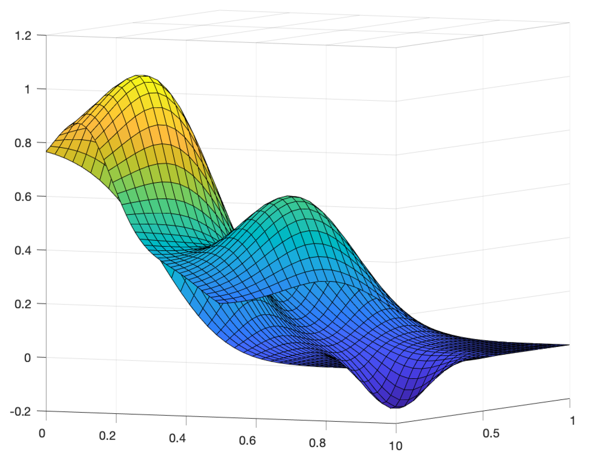
Figure 2.
RMSEs versus number of data sites (). (a) Comparison between SPH and ISPH; (b) comparison between SPH and E-ISPH. All the computations are with starting normalized values and .
Figure 2.
RMSEs versus number of data sites (). (a) Comparison between SPH and ISPH; (b) comparison between SPH and E-ISPH. All the computations are with starting normalized values and .


Figure 3.
RMSEs versus number of data sites (). (a) Comparison between SPH and ISPH; (b) comparison between SPH and E-ISPH. All the computations are with starting normalized values and .
Figure 3.
RMSEs versus number of data sites (). (a) Comparison between SPH and ISPH; (b) comparison between SPH and E-ISPH. All the computations are with starting normalized values and .

Figure 4.
RMSEs versus number of data sites. Comparison between ISPH and E-ISPH. (a) ; (b) . Full line is for ISPH and dashed line is for E-ISPH. All the computations are with starting normalized values and .
Figure 4.
RMSEs versus number of data sites. Comparison between ISPH and E-ISPH. (a) ; (b) . Full line is for ISPH and dashed line is for E-ISPH. All the computations are with starting normalized values and .

Figure 5.
Comparison between ISPH and E-ISPH. (a) Time (s) versus number of data sites; (b) RMSEs versus number of data sites. All the computations are with starting normalized values, as data sites, n = 1000 for ISPH and n = 10 for E-ISPH.
Figure 5.
Comparison between ISPH and E-ISPH. (a) Time (s) versus number of data sites; (b) RMSEs versus number of data sites. All the computations are with starting normalized values, as data sites, n = 1000 for ISPH and n = 10 for E-ISPH.


Table 1.
RMSEs for SPH (standard formulation) and with p = 1. Data sites and .
| N | SPH | = 1 | SPH | = 1 |
| 9 | 0.3487 | 0.2656 | 0.3376 | 0.2624 |
| 25 | 0.3136 | 0.1234 | 0.2885 | 0.2206 |
| 81 | 0.2456 | 0.1617 | 0.2024 | 0.1244 |
| 289 | 0.1540 | 0.0880 | 0.1215 | 0.0693 |
| 1089 | 0.0867 | 0.0403 | 0.0720 | 0.0266 |
| 4225 | 0.0621 | 0.0149 | 0.0605 | 0.0137 |
| 16641 | 0.0545 | 0.0054 | 0.0541 | 0.0046 |
| 66049 | 0.0537 | 0.0023 | 0.0540 | 0.0018 |
Table 2.
RMSEs for ISPH, with p = 1. Data sites .
| N | ||||
|---|---|---|---|---|
| 9 | 0.2656 | 0.1657 | 0.1455 | 0.1834 |
| 25 | 0.1234 | 0.1355 | 0.1156 | 0.0905 |
| 81 | 0.1617 | 0.0919 | 0.0525 | 0.0396 |
| 289 | 0.0880 | 0.0255 | 0.0081 | 0.0042 |
| 1089 | 0.0403 | 0.0030 | 2.91 | 5.51 |
| 4225 | 0.0149 | 9.94 | 1.16 | 1.29 |
Table 3.
RMSEs for the ISPH, with p = 1. Data sites .
| N | ||||
|---|---|---|---|---|
| 9 | 0.2624 | 0.1626 | 0.1427 | 0.1280 |
| 25 | 0.2206 | 0.1331 | 0.1023 | 0.0839 |
| 81 | 0.1244 | 0.0603 | 0.0269 | 0.0167 |
| 289 | 0.0693 | 0.0133 | 0.0042 | 0.0021 |
| 1089 | 0.0266 | 0.0017 | 2.35 | 4.60 |
| 4225 | 0.0137 | 9.15 | 1.27 | 1.71 |
Table 4.
RMSEs for the E-ISPH, with p = 1. Data sites .
| N | |||||
|---|---|---|---|---|---|
| 9 | 0.2656 | 0.1684 | 0.2239 | 0.2247 | 0.2247 |
| 25 | 0.1234 | 0.0963 | 0.1365 | 0.1245 | 0.1375 |
| 81 | 0.1617 | 0.0406 | 0.0241 | 0.0439 | 0.0503 |
| 289 | 0.0880 | 0.0052 | 0.0019 | 0.0022 | 0.0062 |
| 1089 | 0.0403 | 7.87 | 4.18 | 9.56 | 3.19 |
| 4225 | 0.0149 | 2.45 | 3.84 | 5.89 | 3.99 |
Table 5.
RMSEs for the E-ISPH, with p = 1. Data sites .
| N | |||||
|---|---|---|---|---|---|
| 9 | 0.2624 | 0.1312 | 0.3210 | 0.3210 | 0.3210 |
| 25 | 0.2206 | 0.0861 | 0.2719 | 0.3173 | 0.3173 |
| 81 | 0.1244 | 0.0172 | 0.0545 | 0.0435 | 0.0446 |
| 289 | 0.0693 | 0.0023 | 0.0011 | 0.0009 | 0.0013 |
| 1089 | 0.0266 | 6.95 | 2.64 | 9.78 | 7.43 |
| 4225 | 0.0137 | 3.13 | 1.74 | 1.31 | 3.17 |
Publisher’s Note: MDPI stays neutral with regard to jurisdictional claims in published maps and institutional affiliations. |
© 2021 by the author. Licensee MDPI, Basel, Switzerland. This article is an open access article distributed under the terms and conditions of the Creative Commons Attribution (CC BY) license (http://creativecommons.org/licenses/by/4.0/).
Share and Cite
MDPI and ACS Style
Francomano, E. Enhancing the Iterative Smoothed Particle Hydrodynamics Method. Appl. Sci. 2021, 11, 2628. https://doi.org/10.3390/app11062628
AMA Style
Francomano E. Enhancing the Iterative Smoothed Particle Hydrodynamics Method. Applied Sciences. 2021; 11(6):2628. https://doi.org/10.3390/app11062628
Chicago/Turabian StyleFrancomano, Elisa. 2021. "Enhancing the Iterative Smoothed Particle Hydrodynamics Method" Applied Sciences 11, no. 6: 2628. https://doi.org/10.3390/app11062628
Note that from the first issue of 2016, this journal uses article numbers instead of page numbers. See further details here.