
Instability Study of Magnetic Journal Bearing under S-CO2 Condition


Abstract
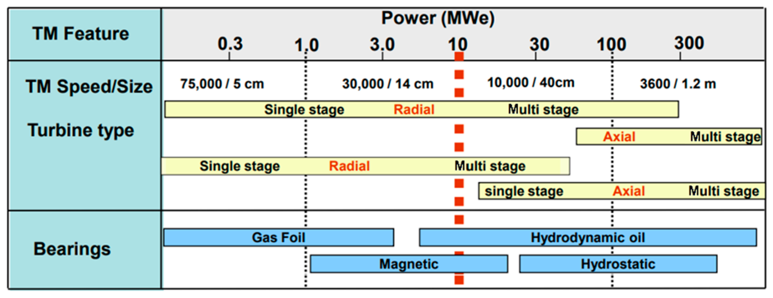
:1. Introduction
2. Magnetic Bearing Analysis for Instability Study
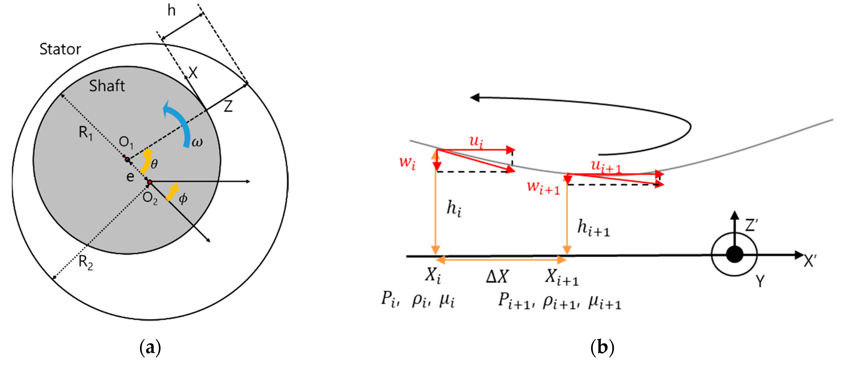
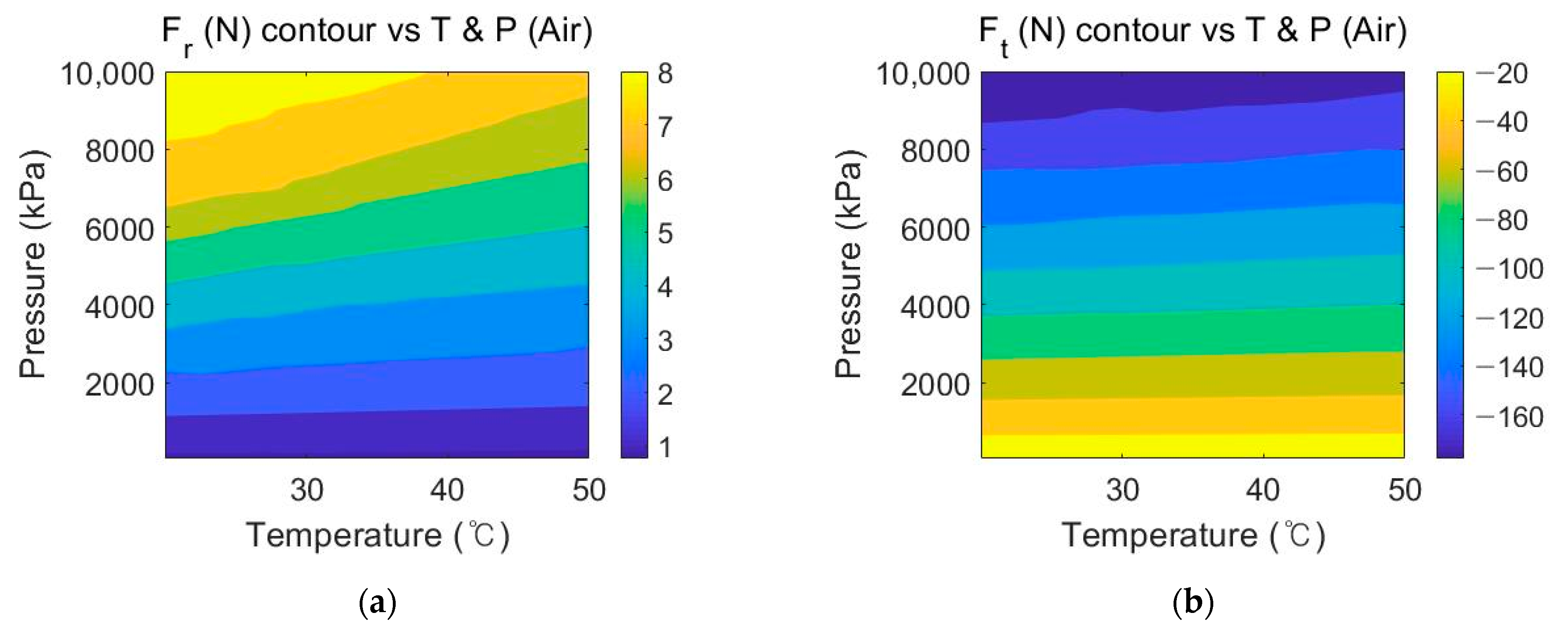
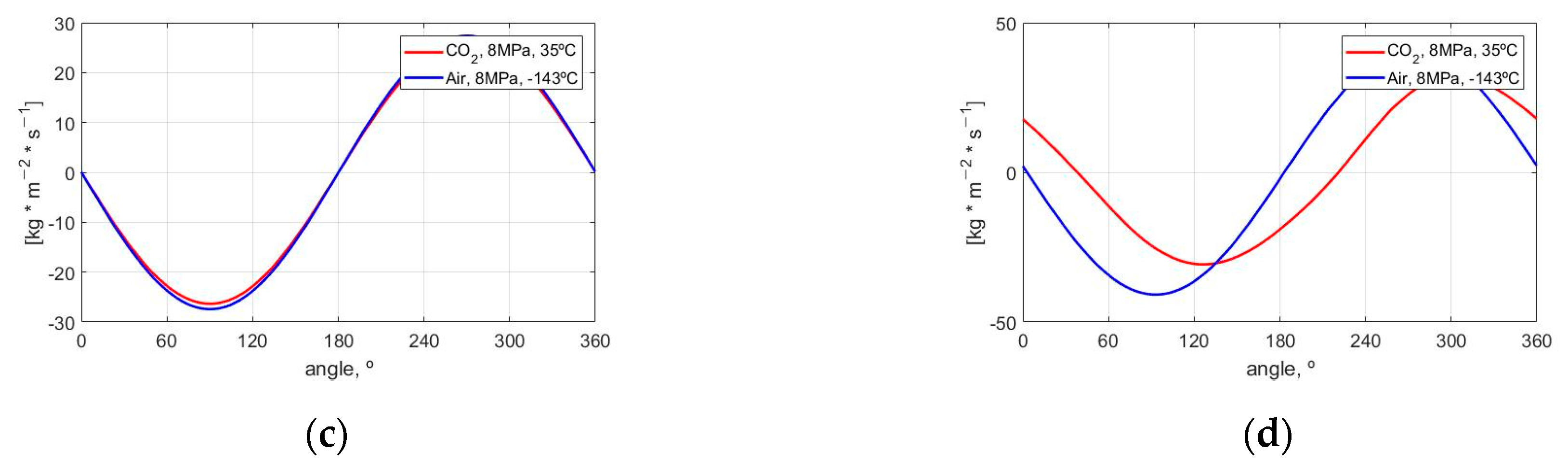
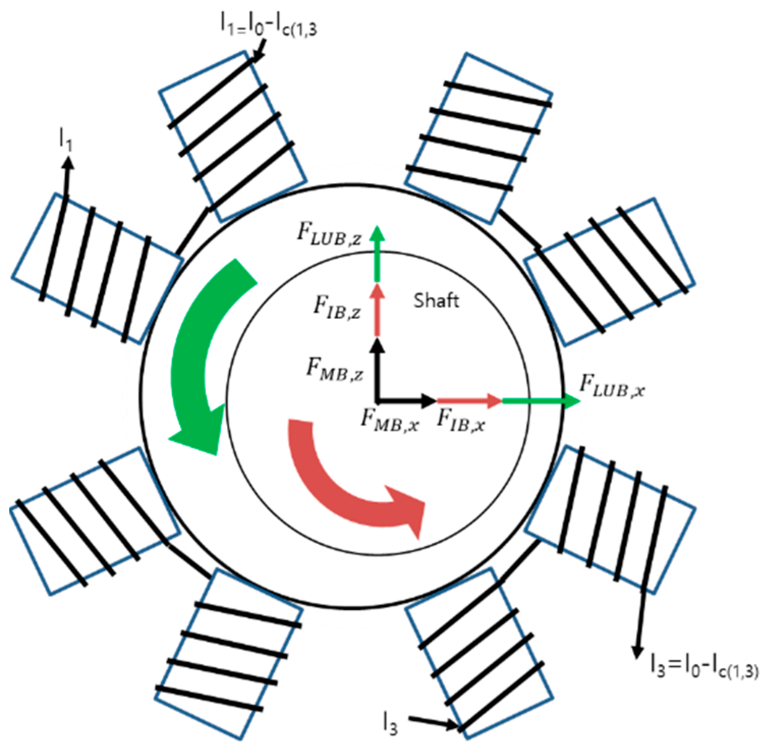
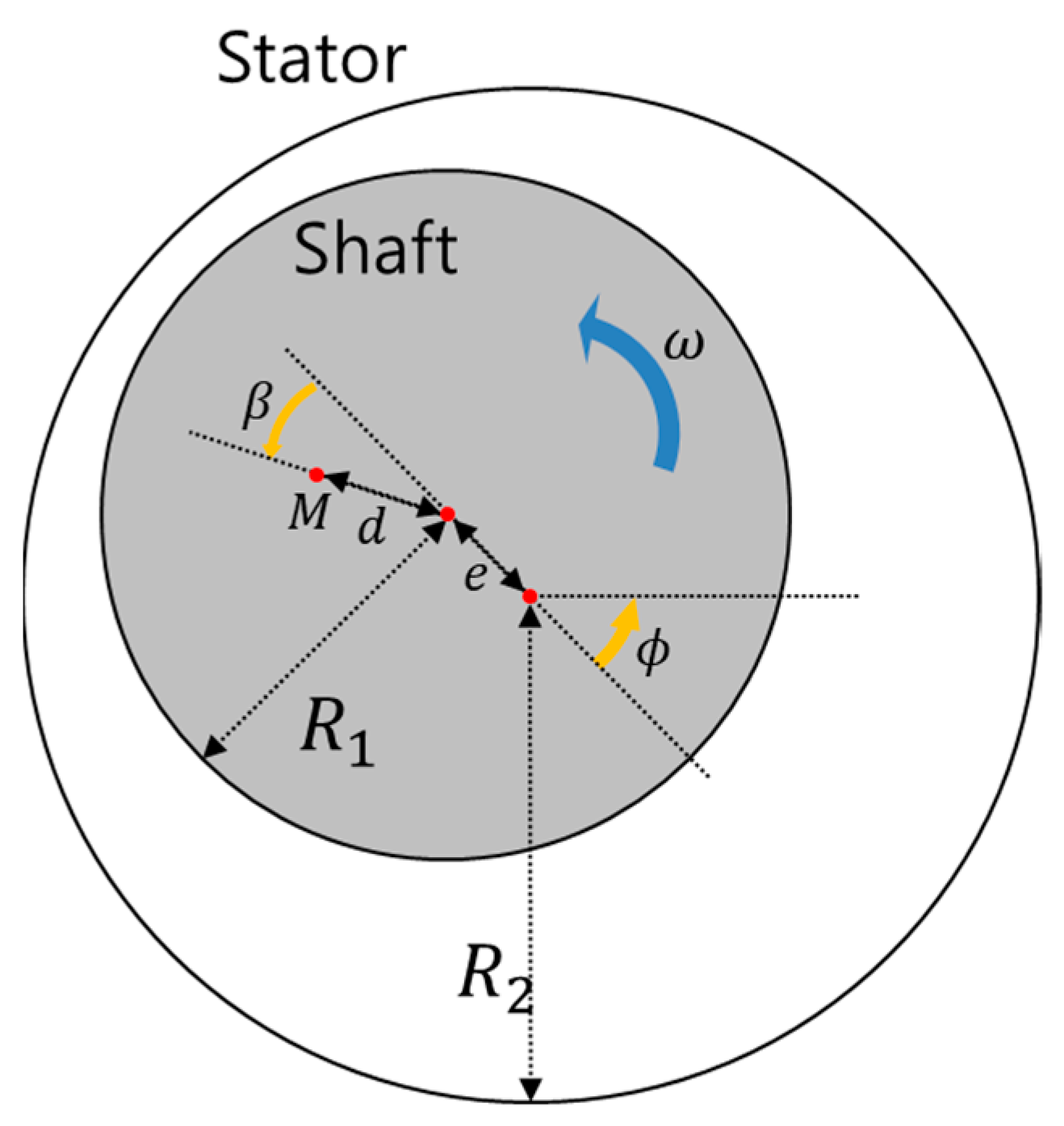
2.1. Magnetic Bearing Lubrication Model Development
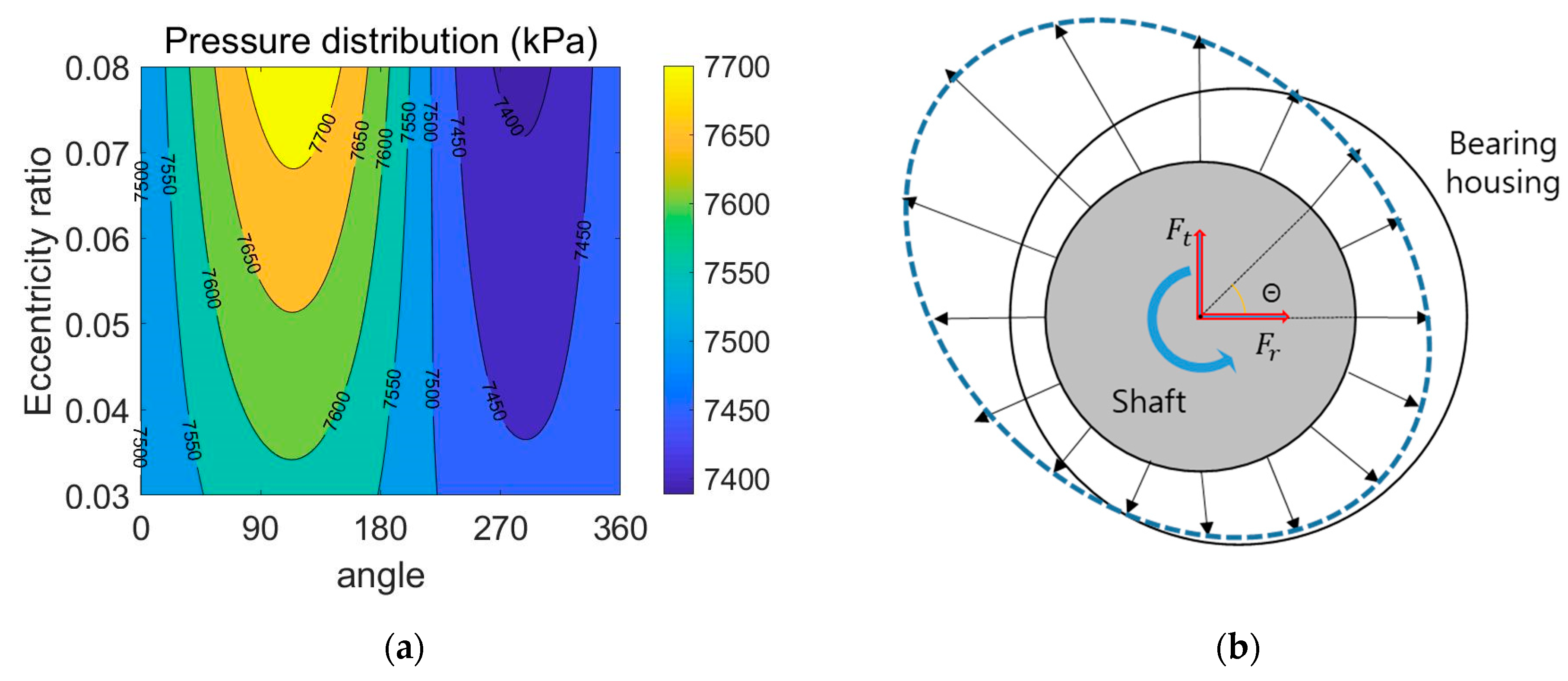
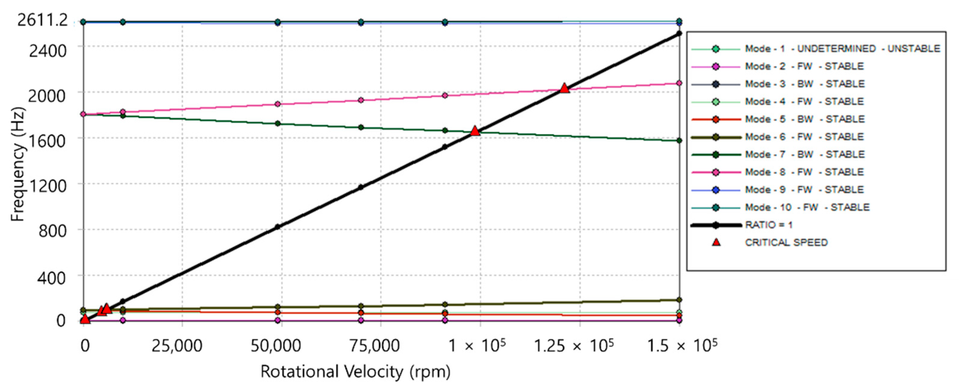
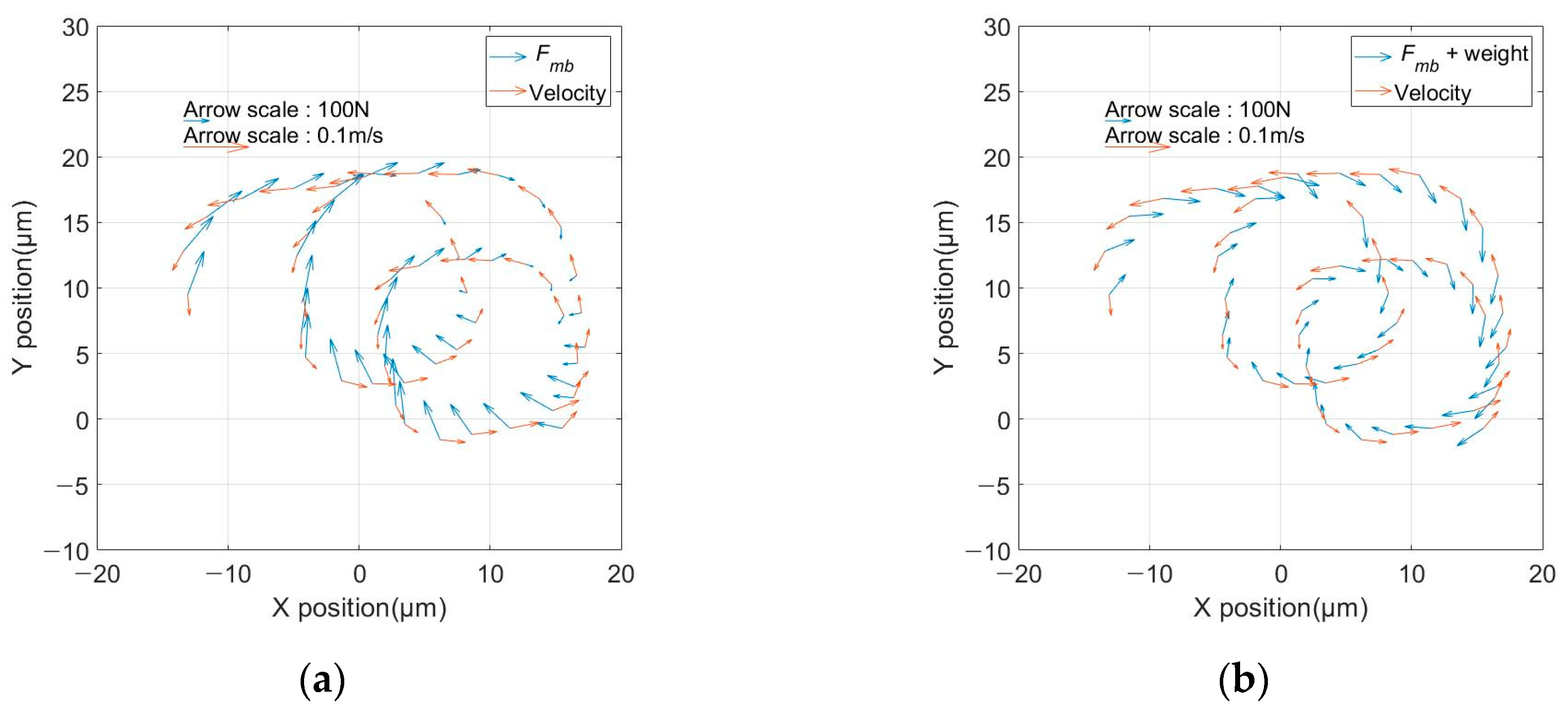
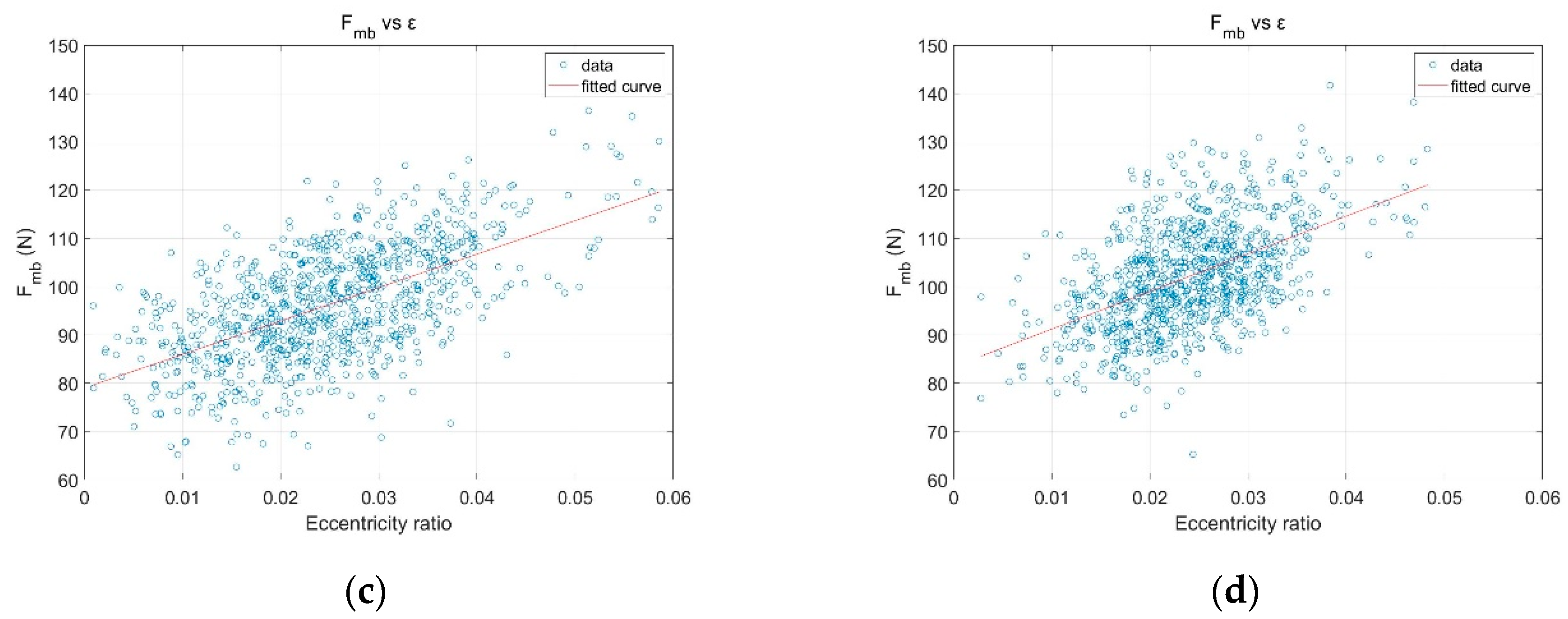
2.2. Magnetic Bearing Lubrication Model Analysis
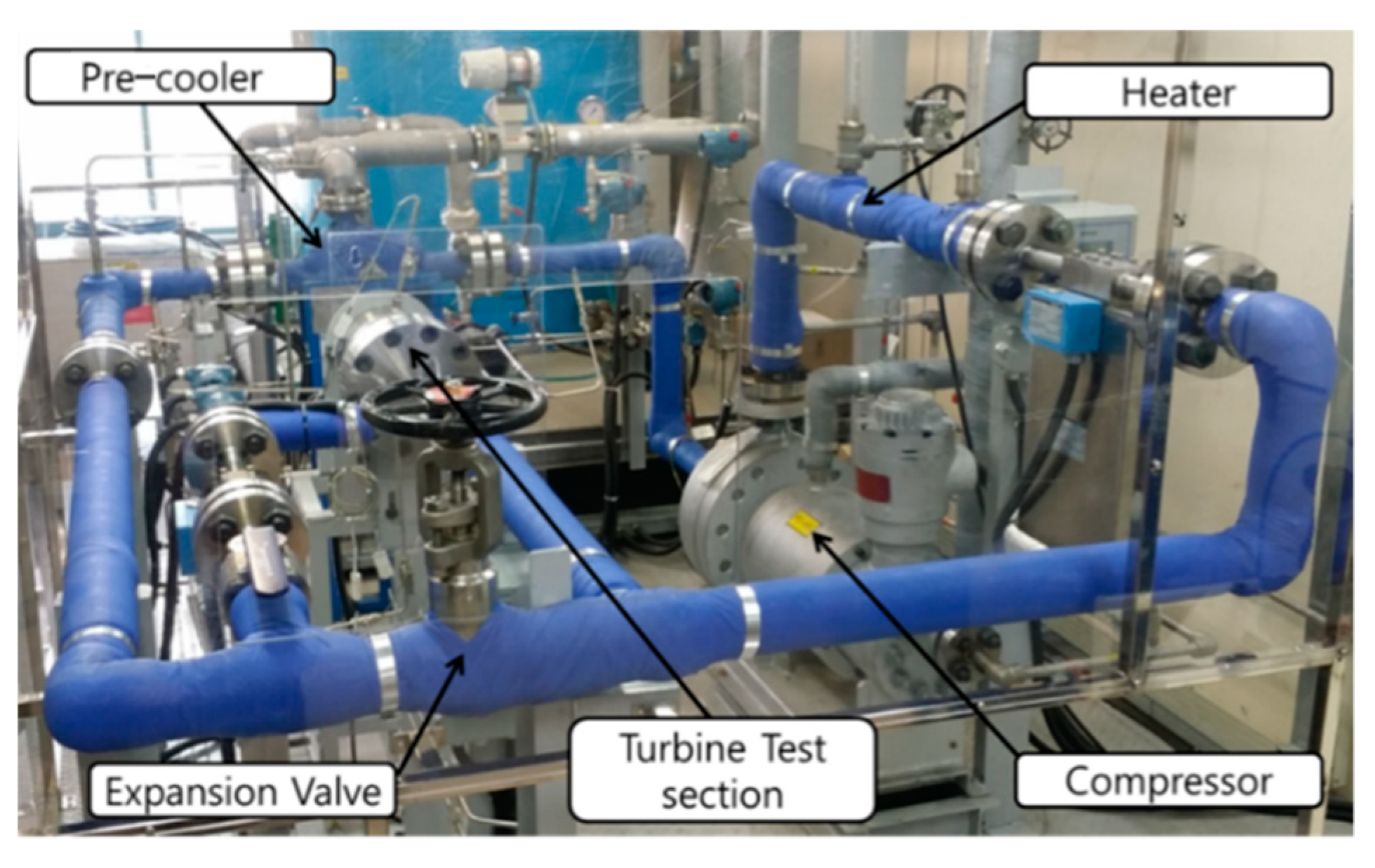
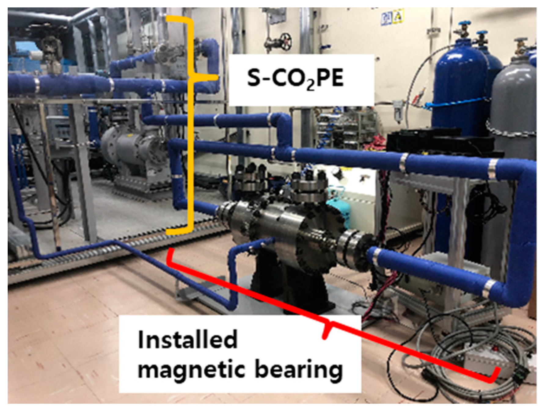
3. Experiments with Magnetic Bearings Under S-CO2 Conditions
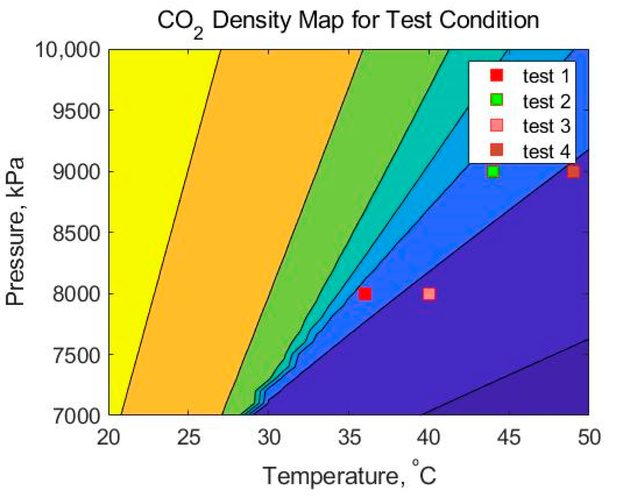
3.1. Magnetic Bearing Experiment
3.2. Data Analysis Method
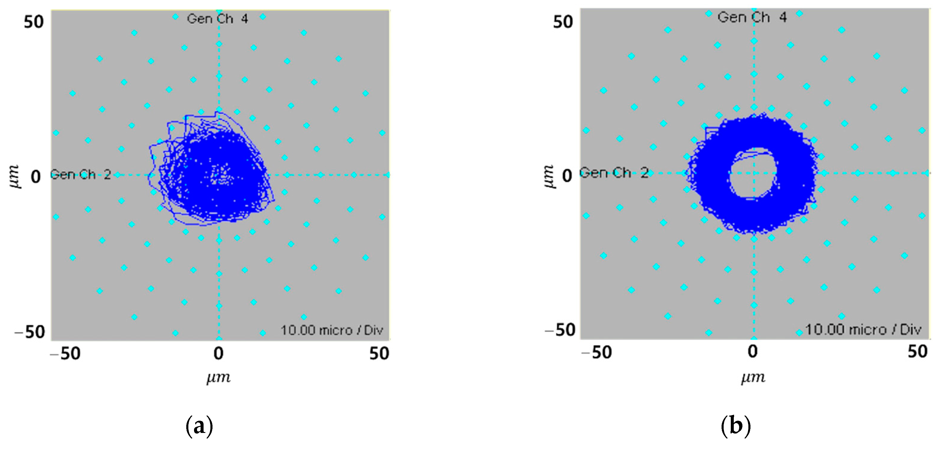
3.3. Results
4. Summary and Discussion
Author Contributions
Funding
Institutional Review Board Statement
Informed Consent Statement
Data Availability Statement
Conflicts of Interest
References
- Dostal, V.; Driscoll, M.; Hejzlar, P. A Supercritical Carbon Dioxide Cycle for Next Generation Nuclear Reactors. Ph.D. Thesis, Massachusetts Institute of Technology, Cambridge, MA, USA, 2004. [Google Scholar]
- Moroz, L.; Burlaka, M.; Rudenko, O. Study of a Supercritical CO2 Power Cycle Application in a Cogeneration Power Plant. In Proceedings of the Supercritical CO2 Power Cycle Symposium, Pittburgh, PA, USA, 9–10 September 2014. [Google Scholar]
- Heshmat, H.; Walton, J.; Córdova, J.L. Technology Readiness of 5th and 6th Generation Compliant Foil Bearing for 10 MWE s-CO2 Turbomachinery Systems. In Proceeding of the 6th International Supercritical CO2 Power Cycles Symposium, Pittsburg, PA, USA, 27–29 March 2018. [Google Scholar]
- Wright, S.A.; Conboy, T.M.; Rochau, G.E. Supercritical CO2 Power Cycle Development Summary at Sandia National Laboratories; Sandia National Labaratories (SNL-NM): Albuquerque, NM, USA, 2011. [Google Scholar]
- Tsuji, T.; Namikawa, D.; Hiaki, T.; Ito, M. Solubility and Liquid Density Measurement for CO2+ Lubricant at High Pressures. In Proceedings of the Asian Pacific Confederation of Chemical Engineering Congress Program and Abstracts, Kitakyushu, Japan, 1 January 2004; The Society of Chemical Engineers: Kitakyushu, Japan, 2004. [Google Scholar]
- Seeton, C.J.; Hrnjak, P. Thermophysical Properties of CO2-lubricant Mixtures and Their Affect on 2-phase Flow in Small Channels (Less than 1mm). In Proceedings of the International Refrigeration and Air Conditioning Conference at Purdue, West Lafayette, IN, USA, 17–20 July 2006. [Google Scholar]
- Srinivas, R.S.; Tiwari, R.; Kannababu, C. Application of Active Magnetic Bearings in Flexible Rotordynamic Systems–A State-of-the-art Review. Mech. Syst. Signal Process. 2018, 106, 537–572. [Google Scholar] [CrossRef]
- Onuma, H.; Masuzawa, T.; Okada, Y. Hybrid Magnetic Bearing. U.S. Patent 7,683,514, 2010. [Google Scholar]
- Zhu, R.; Xu, W.; Ye, C.; Zhu, J. Novel Heteropolar Radial Hybrid Magnetic Bearing with Low Rotor Core Loss. IEEE Trans. Magn. 2017, 53, 1–5. [Google Scholar] [CrossRef]
- Chen, H.; Jiang, B.; Ding, S.X.; Huang, B. Data-Driven Fault Diagnosis for Traction Systems in High-Speed Trains: A Survey, Challenges, and Perspectives. IEEE Trans. Intell. Transp. Syst. 2020, 1–17. [Google Scholar] [CrossRef]
- Cha, J.E.; Cho, S.K.; Lee, J.; Lee, J.I. Supercritical CO2 Compressor with Active Magnetic Bearing. In Proceedings of the Transactions of the Korean Nuclear Society Spring Meeting, Jeju, Korea, 11–13 May 2016. [Google Scholar]
- Kim, D.; Baik, S.; Lee, J.I. Frequency Analysis of Magnetic Journal Bearing Instability for MMR Condition. In Proceedings of the Transactions of the Korean Nuclear Society Virtual Spring Meeting, 9–10 July 2020. [Google Scholar]
- Sun, J.; Wei, W.; Tang, J.; Wang, C.-E. Dynamic Stiffness Analysis and Experimental Verification of Axial Magnetic Bearing Based on Air Gap Flux Variation in Magnetically Suspended Molecular Pump. Chin. J. Mech. Eng. 2020, 33, 1–11. [Google Scholar] [CrossRef]
- Chao, Q.; Zhang, J.; Xu, B.; Wang, Q. Discussion on the Reynolds Equation for the Slipper Bearing Modeling in Axial Piston Pumps. Tribol. Int. 2018, 118, 140–147. [Google Scholar] [CrossRef]
- Snyder, T.; Braun, M. Comparison of Perturbed Reynolds Equation and CFD Models for the Prediction of Dynamic Coefficients of Sliding Bearings. Lubricants 2018, 6, 5. [Google Scholar] [CrossRef] [Green Version]
- Mahner, M.; Bauer, M.; Schweizer, B. Numerical Analyzes and Experimental Investigations on the Fully-coupled Thermo-elasto-gasdynamic Behavior of Air Foil Journal Bearings. Mech. Syst. Signal Process. 2021, 149, 107221. [Google Scholar] [CrossRef]
- Liu, Y.; Ming, S.; Zhao, S.; Han, J.; Ma, Y. Research on Automatic Balance Control of Active Magnetic Bearing-Rigid Rotor System. Shock. Vib. 2019, 2019, 1–13. [Google Scholar] [CrossRef]
- Hamrock, B.J.; Schmid, S.R.; Jacobson, B.O. Fundamentals of Fluid Film Lubrication; CRC Press: Boca Raton, FL, USA, 2004; Volume 169. [Google Scholar]
- Szeri, A.Z.; Rohde, S.M. Tribology: Friction, Lubrication, and Wear. J. Lubr. Technol. 1981, 103, 320. [Google Scholar] [CrossRef] [Green Version]
- Taylor, C.M.; Dowson, D. Turbulent Lubrication Theory—Application to Design. J. Lubr. Technol. 1974, 96, 36–46. [Google Scholar] [CrossRef]
- Dousti, S.; Allaire, P. A Compressible Hydrodynamic Analysis of Journal Bearings Lubricated with Supercritical Carbon Dioxide. In Proceeding of Supercritical CO2 Power Cycle Symposium, San Antonio, TX, USA, 29–31 March 2016. [Google Scholar]
- Gunter, E.J. Understanding Amplitude and Phase in Rotating Machinery. In Proceedings of the Vibration Institute 33rd Annual Meeting, Harrisburg, PA, USA, 23–27 June 2009. [Google Scholar]
- Ertas, B.; Vance, J. The Influence of Same-Sign Cross-Coupled Stiffness on Rotordynamics. J. Vib. Acoust. 2006, 129, 24–31. [Google Scholar] [CrossRef]


| Thermal Condition | ||
|---|---|---|
| Air at 8 MPa, −153.7 °C | 35.3 | −1433.6 |
| CO2 at 8 MPa, 30 °C | 265.2 | −1344.7 |
Publisher’s Note: MDPI stays neutral with regard to jurisdictional claims in published maps and institutional affiliations. |
© 2021 by the authors. Licensee MDPI, Basel, Switzerland. This article is an open access article distributed under the terms and conditions of the Creative Commons Attribution (CC BY) license (https://creativecommons.org/licenses/by/4.0/).
Share and Cite
Kim, D.; Baik, S.; Lee, J. Instability Study of Magnetic Journal Bearing under S-CO2 Condition. Appl. Sci. 2021, 11, 3491. https://doi.org/10.3390/app11083491
Kim D, Baik S, Lee J. Instability Study of Magnetic Journal Bearing under S-CO2 Condition. Applied Sciences. 2021; 11(8):3491. https://doi.org/10.3390/app11083491
Chicago/Turabian StyleKim, Dokyu, SeungJoon Baik, and JeongIk Lee. 2021. "Instability Study of Magnetic Journal Bearing under S-CO2 Condition" Applied Sciences 11, no. 8: 3491. https://doi.org/10.3390/app11083491