
The Inversion Analysis and Material Parameter Optimization of a High Earth-Rockfill Dam during Construction Periods


Abstract
:1. Introduction
2. Briefings on the Inversion Method for Earth-Rockfill Dams during Construction Periods
2.1. Constitutive Model and Inversion Parameters Selection
2.2. Conventional Inversion Method Based on the BP Neural Network
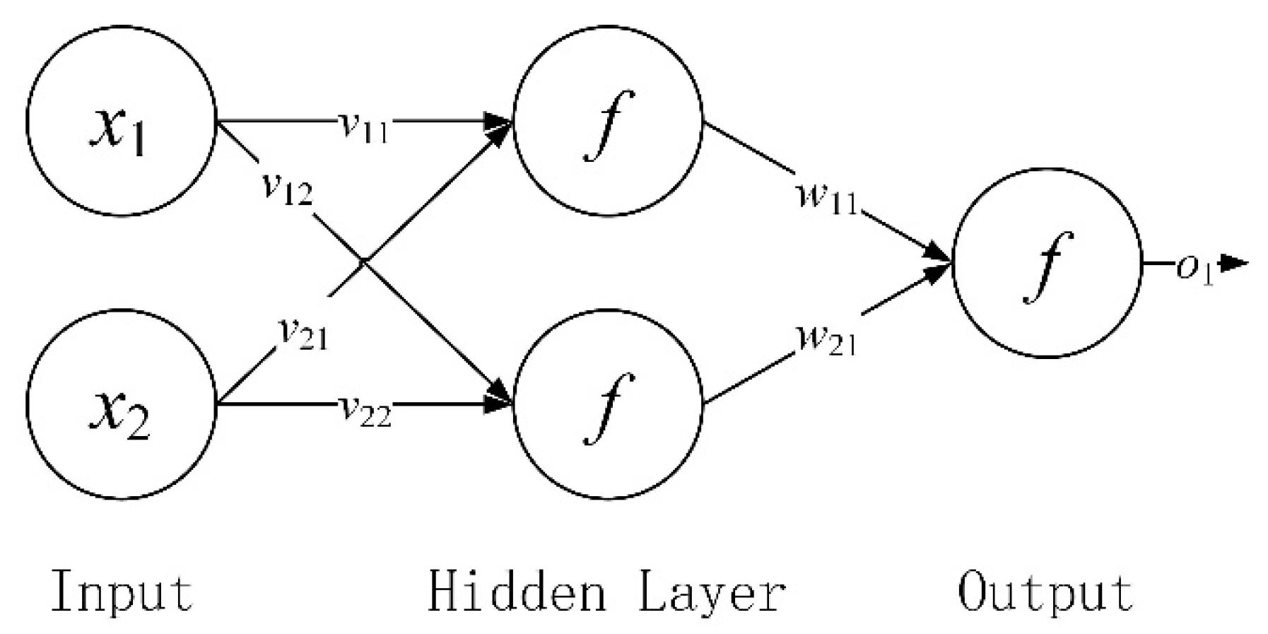
2.2.1. Back Propagation Neural Network
2.2.2. Conventional Inversion Process
3. Step-by-Step Inversion Method
4. Numerical Examples
4.1. Benchmark Problem: Simple Inversion Analysis Based on the Results of Forward Analysis
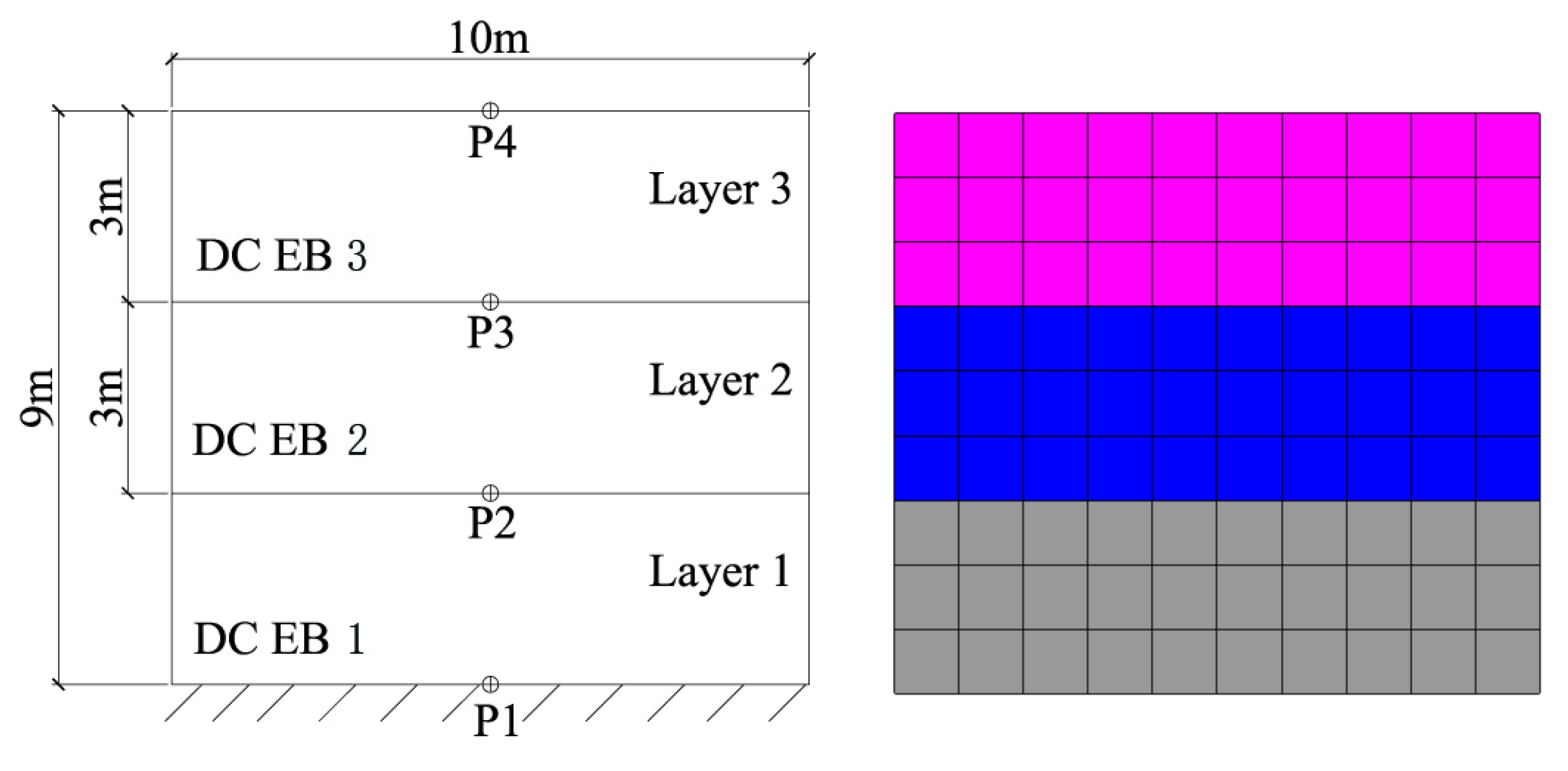
4.1.1. Problem Description
4.1.2. Forward Analysis and Assumed Monitoring Data
4.1.3. Validation Checks of Conventional and Step-by-Step Inversion Analysis
4.2. Inversion Analysis of a High Earth-Rockfill Dam Using the Step-by-Step Method
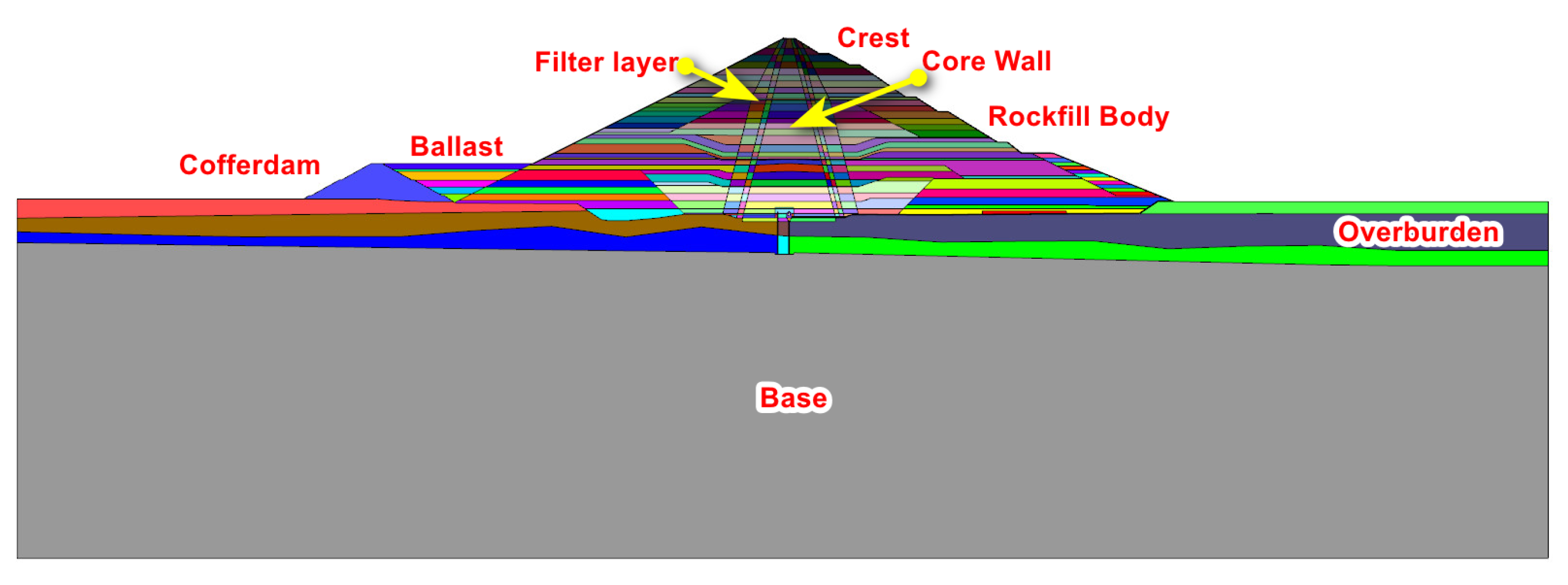
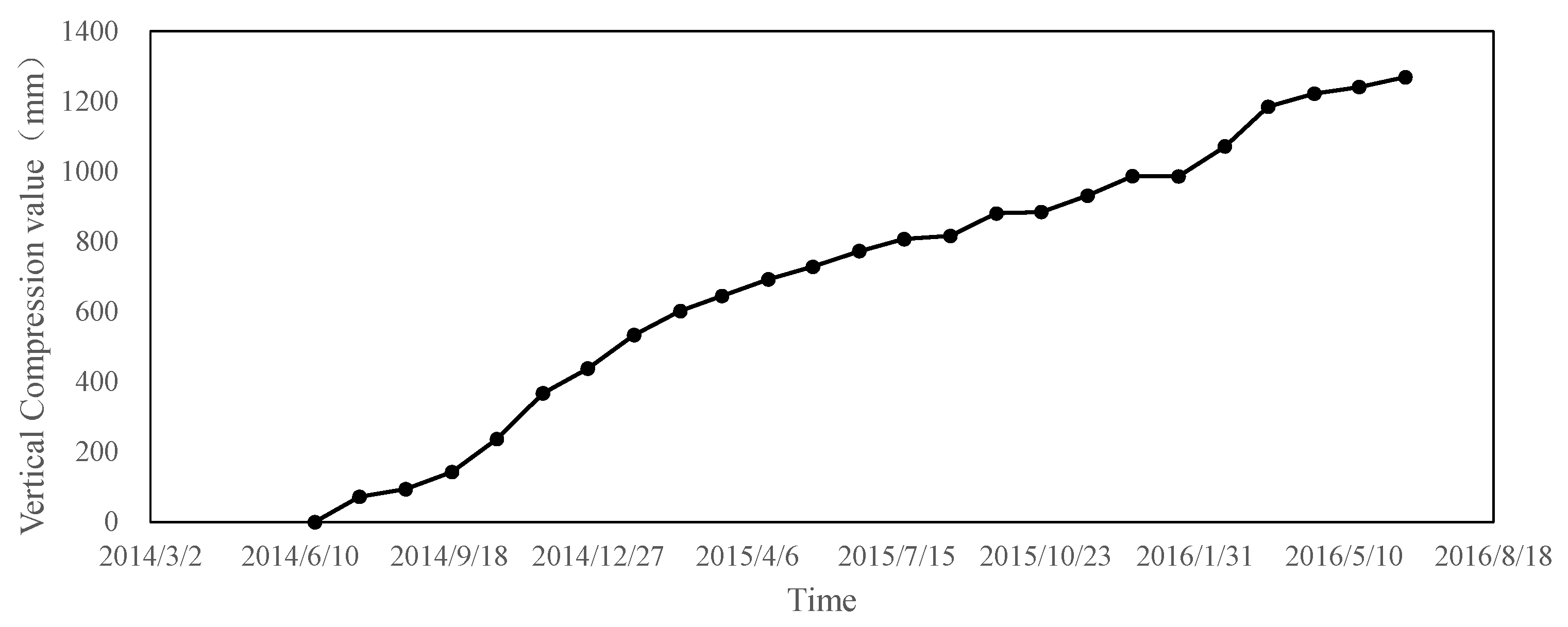
4.2.1. Problem Description
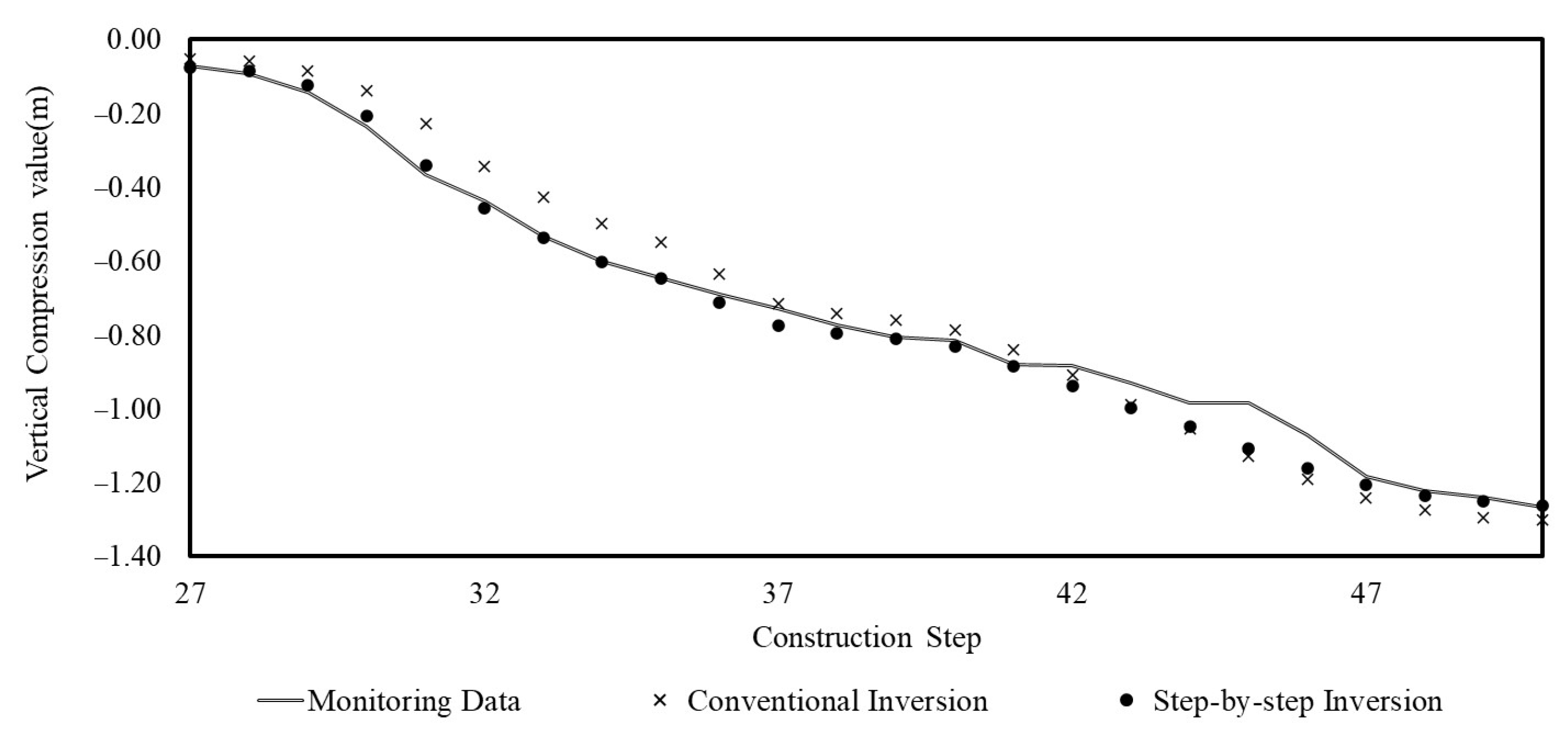
4.2.2. Step-by-Step Inversion Analysis
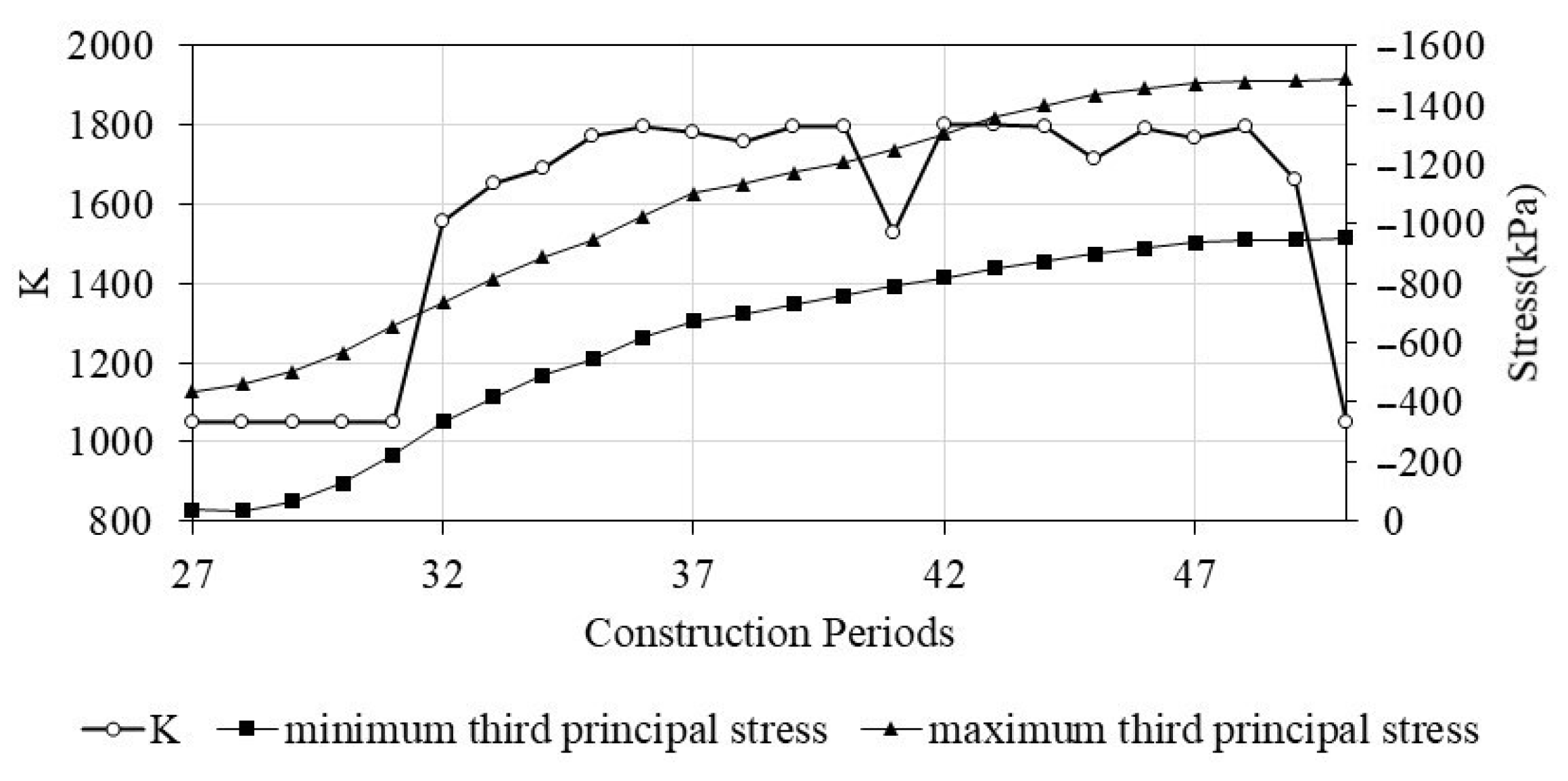
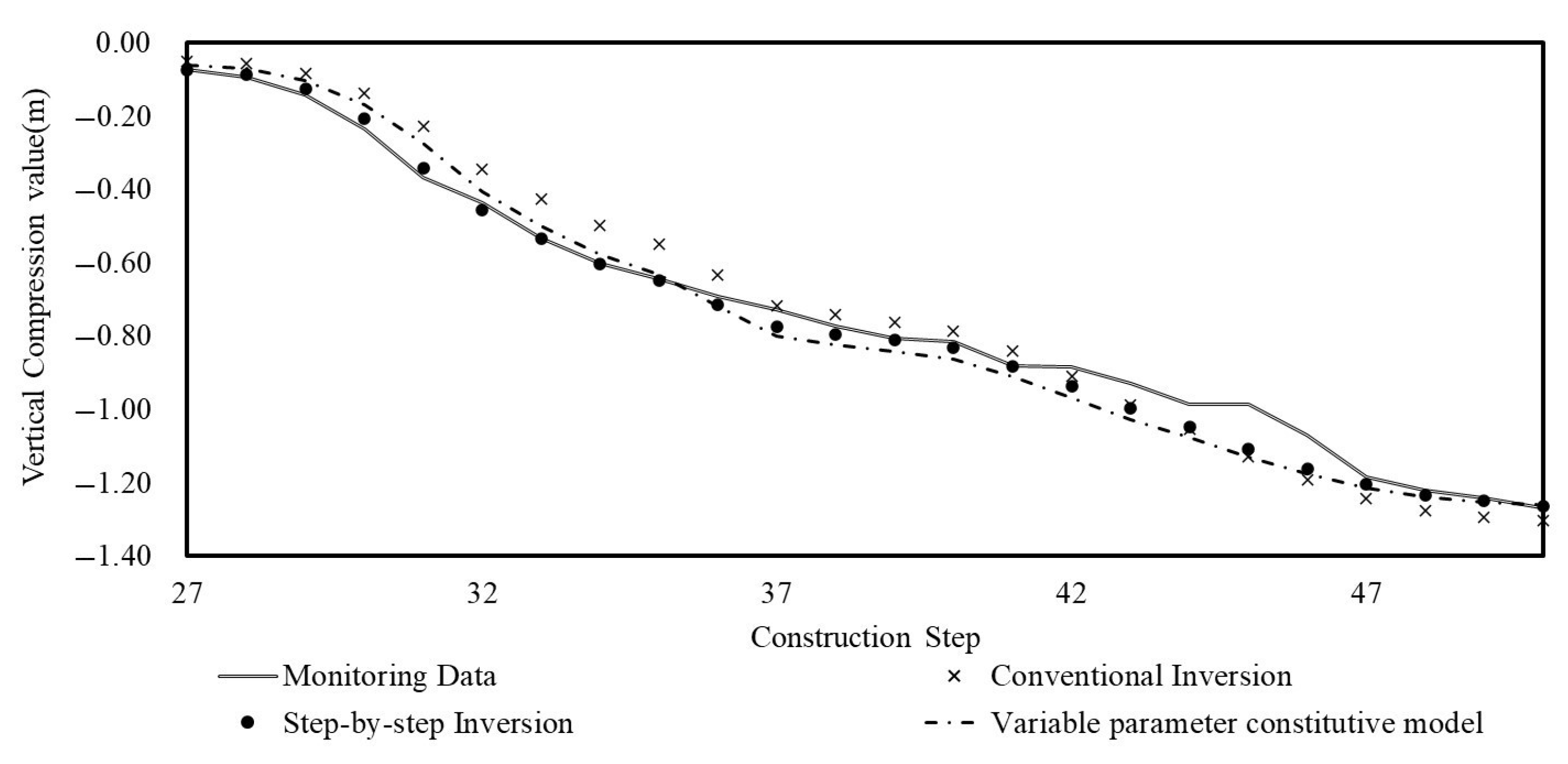
4.2.3. Further Study on Material Parameter Optimization
5. Discussion and Conclusions
5.1. Discussion
5.2. Conclusions
Author Contributions
Funding
Institutional Review Board Statement
Informed Consent Statement
Data Availability Statement
Conflicts of Interest
References
- Li, X.; Li, Y.; Lu, X.; Wang, Y.; Zhang, H.; Zhang, P. An online anomaly recognition and early warning model for dam safety monitoring data. Struct. Health Monit. 2020, 19, 1475–9217. [Google Scholar] [CrossRef]
- Zhong, D.; Li, X.; Cui, B.; Wu, B.; Liu, Y. Technology and application of real-time compaction quality monitoring for earth-rockfill dam construction in deep narrow valley. Autom. Constr. 2018, 90, 23–38. [Google Scholar] [CrossRef]
- Li, X.; Wen, Z.; Su, H. An approach using random forest intelligent algorithm to construct a monitoring model for dam safety. Eng. Comput. 2021, 37, 39–56. [Google Scholar] [CrossRef]
- Khoroshilov, V.; Kobeleva, N.; Noskov, M. Analysis of Possibilities to Use Predictive Mathematical Models for Studying the Dam Deformation State. J. Appl. Comput. Mech. 2022, 8, 733–744. [Google Scholar]
- Ma, C.; Yang, J.; Cheng, L.; Ran, L. Adaptive parameter inversion analysis method of rockfill dam based on harmony search algorithm and mixed multi-output relevance vector machine. Eng. Comput. 2020, 37, 2229–2249. [Google Scholar] [CrossRef]
- Kang, F.; Liu, X.; Li, J.; Li, H. Multi-parameter inverse analysis of concrete dams using kernel extreme learning machines-based response surface model. Eng. Struct. 2022, 256, 0141–0296. [Google Scholar] [CrossRef]
- Yang, X.S.; Gandomi, A.H. Bat Algorithm: A Novel Approach for Global Engineering Optimization. Eng. Comput. 2012, 29, 464–483. [Google Scholar] [CrossRef] [Green Version]
- Bi, W.; Xu, Y.; Wang, H. Comparison of Searching Behaviour of Three Evolutionary Algorithms Applied to Water Distribution System Design Optimization. Water 2020, 12, 695. [Google Scholar] [CrossRef] [Green Version]
- Gong, W.; Tian, S.; Wang, L.; Li, Z.; Tang, H.; Li, T.; Zhang, L. Interval prediction of landslide displacement with dual-output least squares support vector machine and particle swarm optimization algorithms. Acta Geotech. 2022, 17. [Google Scholar] [CrossRef]
- Song, T.; Ding, W.; Liu, H.; Wu, J.; Zhou, H.; Chu, J. Uncertainty Quantification in Machine Learning Modeling for Multi-Step Time Series Forecasting: Example of Recurrent Neural Networks in Discharge Simulations. Water 2020, 12, 912. [Google Scholar] [CrossRef] [Green Version]
- Pan, S.Y.; Cheng, J.; Li, T.C. The forward and inversion analysis of high rock-fill dam during construction period using the node-based smoothed point interpolation method. Eng. Comput. 2020, 37, 1531–1555. [Google Scholar] [CrossRef]
- Wang, M.; Chi, S.; Xie, Y.; Zhou, X. Dynamic parameters inversion analysis of rockfill materials considering interaction effects based on weak earthquakes. Soil Dyn. Earthq. Eng. 2020, 130, 0267–7261. [Google Scholar] [CrossRef]
- Zhou, X.; Sun, X.; Zheng, J.; Jiang, H.; Li, Y.; Li, Z.; Ma, Z.; Cao, P.; Zhan, Q.; Zhao, Y. Long-term settlement of high concrete-face rockfill dam by field monitoring and numerical simulation. Adv. Civ. Eng. 2020, 2020, 1687–8086. [Google Scholar] [CrossRef]
- Li, J.; Cheng, J.-H.; Shi, J.-Y.; Huang, F. Brief introduction of back propagation (BP) neural network algorithm and its improvement. In Advances in Computer Science and Information Engineering; Springer: Berlin, Germany, 2012; pp. 553–558. [Google Scholar]
- Li, G.; Hu, Y.; Li, Q.B.; Yin, T.; Miao, J.X.; Yao, M. Inversion Method of In-situ Stress and Rock Damage Characteristics in Dam Site Using Neural Network and Numerical Simulation—A Case Study. IEEE Access 2020, 8, 46701–46712. [Google Scholar] [CrossRef]
- Zhou, X.; Sun, X.; Li, Y.; Zhang, J.; Li, Z.; Ma, Z.; Guan, Z.; Zhang, Y.; Zhang, P. Creep parameter inversion for high CFRDs based on improved BP neural network response surface method. Soft Comput. 2022. [Google Scholar] [CrossRef]
- Dong, W.; Hu, L.; Yu, Y.Z.; Lv, H. Comparison between Duncan and Chang’s EB model and the generalized plasticity model in the analysis of a high earth-rockfill dam. J. Appl. Math. 2013, 2013, 709430. [Google Scholar] [CrossRef] [Green Version]
- JM, D. Nonlinear Analysis of Stress and Strain in Soils. J. Soil Mech. Found. Div. 1970, 96, 1629–1653. [Google Scholar]
- Liu, K.; Chen, S.L.; Voyiadjis, G.Z. Integration of anisotropic modified Cam Clay model in finite element analysis: Formulation, validation, and application. Comput. Geotech. 2019, 116, 103198. [Google Scholar] [CrossRef]
- López-Querol, S.; Fernández-Merodo, J.A.; Mira, P.; Pastor, M. Numerical modelling of dynamic consolidation on granular soils. Int. J. Numer. Anal. Methods Geomech. 2008, 32, 1431–1457. [Google Scholar] [CrossRef]
- Jia, P.; Khoshghalb, A.; Chen, C.; Zhao, W.; Dong, M.; Alipour Esgandani, G. Modified Duncan-Chang constitutive model for modeling supported excavations in granular soils. Int. J. Geomech. 2020, 20, 04020211. [Google Scholar] [CrossRef]
- Zhao, Y.; Ling, X.; Gong, W.; Li, P.; Li, G.; Wang, L. Mechanical Properties of Fiber-Reinforced Soil under Triaxial Compression and Parameter Determination Based on the Duncan-Chang Model. Appl. Sci. 2020, 10, 9043. [Google Scholar] [CrossRef]
- Wang, L.; Xiao, S. Calculation Method for Displacement-Dependent Earth Pressure on a Rigid Wall Rotating Around Its Base. Int. J. Geomech. 2021, 21, 1532–3641. [Google Scholar] [CrossRef]
- Liu, X.-Q.; Liu, J.-K.; Tian, Y.-H.; Chang, D.; Hu, T.-F. Influence of the freeze-thaw effect on the Duncan-Chang model parameter for lean clay. Transp. Geotech. 2019, 21, 2214–3912. [Google Scholar] [CrossRef]
- Xiong, J.H.; Kou, X.Y.; Liu, F.; Jiang, M.J. Applicability of Duncan-Chang model and its modified versions to methane hydrate-bearing sands. Adv. Mater. Res. 2011, 347–353, 3384–3387. [Google Scholar] [CrossRef]


| Layer | Density (kg/m3) | c (kPa) | (kPa) | ||||||||
|---|---|---|---|---|---|---|---|---|---|---|---|
| 1 | 2000 | 40 | 20 | 0.85 | 400 | 0.45 | 150 | 0.25 | 460 | 0 | 101 |
| 2 | 2000 | 40 | 20 | 0.85 | 300 | 0.45 | 150 | 0.25 | 360 | 0 | 101 |
| 3 | 2000 | 40 | 20 | 0.85 | 350 | 0.45 | 150 | 0.25 | 360 | 0 | 101 |
| Sequence | Sequence | ||||||
|---|---|---|---|---|---|---|---|
| 1 | 360 | 0.44 | 0.83 | 42 | 360 | 0.43 | 0.85 |
| 2 | 370 | 0.41 | 0.87 | 43 | 370 | 0.41 | 0.85 |
| 3 | 380 | 0.45 | 0.77 | 44 | 380 | 0.44 | 0.77 |
| 4 | 390 | 0.46 | 0.87 | 45 | 390 | 0.48 | 0.77 |
| 5 | 400 | 0.42 | 0.77 | 46 | 400 | 0.41 | 0.77 |
| 6 | 410 | 0.48 | 0.83 | 47 | 410 | 0.44 | 0.75 |
| 7 | 420 | 0.42 | 0.83 | 48 | 420 | 0.4 | 0.81 |
| 8 | 430 | 0.42 | 0.9 | 49 | 430 | 0.42 | 0.87 |
| 9 | 360 | 0.47 | 0.87 | 50 | 360 | 0.48 | 0.75 |
| 10 | 370 | 0.43 | 0.77 | 51 | 370 | 0.4 | 0.9 |
| 11 | 380 | 0.44 | 0.87 | 52 | 380 | 0.41 | 0.75 |
| 12 | 390 | 0.42 | 0.79 | 53 | 390 | 0.42 | 0.89 |
| 13 | 400 | 0.42 | 0.81 | 54 | 400 | 0.4 | 0.89 |
| 14 | 410 | 0.45 | 0.89 | 55 | 410 | 0.48 | 0.79 |
| 15 | 420 | 0.45 | 0.75 | 56 | 420 | 0.47 | 0.83 |
| 16 | 430 | 0.43 | 0.79 | 57 | 430 | 0.4 | 0.79 |
| 17 | 360 | 0.47 | 0.75 | 58 | 360 | 0.4 | 0.83 |
| 18 | 370 | 0.45 | 0.79 | 59 | 370 | 0.4 | 0.77 |
| 19 | 380 | 0.48 | 0.81 | 60 | 380 | 0.42 | 0.75 |
| 20 | 390 | 0.47 | 0.77 | 61 | 390 | 0.43 | 0.87 |
| 21 | 400 | 0.44 | 0.9 | 62 | 400 | 0.48 | 0.9 |
| 22 | 410 | 0.46 | 0.89 | 63 | 410 | 0.47 | 0.89 |
| 23 | 420 | 0.47 | 0.81 | 64 | 420 | 0.46 | 0.75 |
| 24 | 430 | 0.47 | 0.79 | 65 | 430 | 0.47 | 0.85 |
| 25 | 360 | 0.41 | 0.9 | 66 | 360 | 0.44 | 0.85 |
| 26 | 370 | 0.46 | 0.83 | 67 | 370 | 0.4 | 0.87 |
| 27 | 380 | 0.47 | 0.9 | 68 | 380 | 0.41 | 0.89 |
| 28 | 390 | 0.48 | 0.87 | 69 | 390 | 0.46 | 0.9 |
| 29 | 400 | 0.46 | 0.81 | 70 | 400 | 0.48 | 0.89 |
| 30 | 410 | 0.44 | 0.81 | 71 | 410 | 0.4 | 0.85 |
| 31 | 420 | 0.45 | 0.85 | 72 | 420 | 0.46 | 0.77 |
| 32 | 430 | 0.41 | 0.79 | 73 | 430 | 0.46 | 0.79 |
| 33 | 360 | 0.41 | 0.83 | 74 | 360 | 0.41 | 0.81 |
| 34 | 370 | 0.45 | 0.81 | 75 | 370 | 0.42 | 0.85 |
| 35 | 380 | 0.45 | 0.9 | 76 | 380 | 0.45 | 0.83 |
| 36 | 390 | 0.43 | 0.81 | 77 | 390 | 0.44 | 0.89 |
| 37 | 400 | 0.45 | 0.87 | 78 | 400 | 0.43 | 0.75 |
| 38 | 410 | 0.46 | 0.85 | 79 | 410 | 0.48 | 0.85 |
| 39 | 420 | 0.4 | 0.75 | 80 | 420 | 0.43 | 0.89 |
| 40 | 430 | 0.43 | 0.9 | 81 | 430 | 0.44 | 0.79 |
| 41 | 360 | 0.43 | 0.83 |
| Material Parameters | Conventional Inversion Analysis | Step-by-Step Inversion Analysis | ||
|---|---|---|---|---|
| Construction Period 1 | Construction Period 2 | Construction Period 3 | ||
| K | 400 | 396 | 399 | 395 |
| n | 0.44 | 0.44 | 0.44 | 0.44 |
| Rf | 0.83 | 0.83 | 0.83 | 0.83 |
| Construction Steps | Vertical Displacement of Monitoring Point (m) | Errors between Step-by-Step Inversion Method and Original Data | Errors between Conventional Inversion Method and Original Data | ||
|---|---|---|---|---|---|
| Original Data | Step-by-Step Inversion Method | Conventional Inversion Method | |||
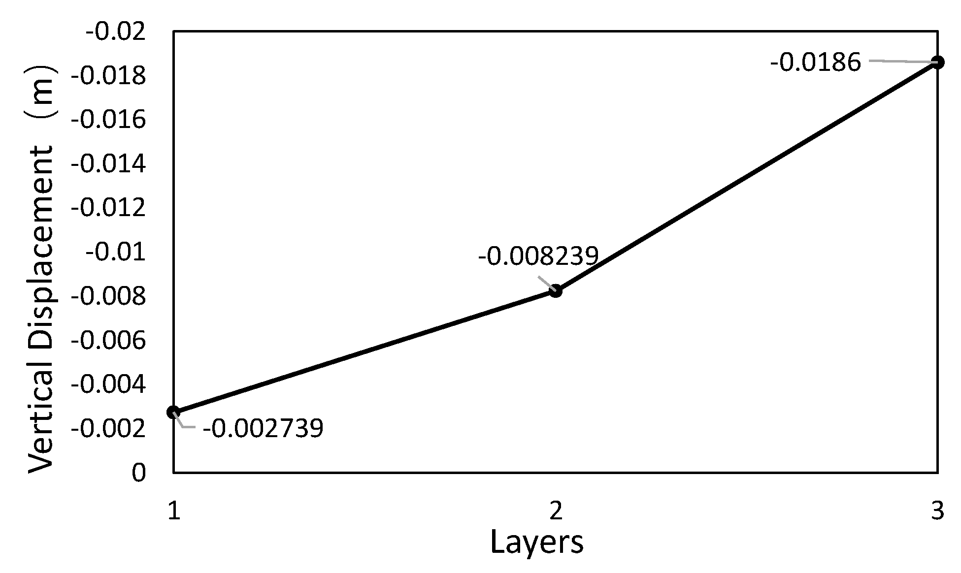
| 1 | −0.00277 | −0.00274 | −0.00277 | −1.19% | −0.13% |
| 2 | −0.00824 | −0.00822 | −0.00819 | −0.23% | −0.56% |
| 3 | −0.01858 | −0.0184 | −0.0183 | −0.94% | −1.47% |
| Sections | Density (t/m3) | C (kPa) | ||||||||
|---|---|---|---|---|---|---|---|---|---|---|
| Overburden | 2.145 | 98 | 38 | 0.83 | 438.263 | 0.39 | 269.26 | 0.39 | 1360 | 5.26 |
| Cofferdam | 2.145 | 98 | 38 | 0.83 | 438.263 | 0.39 | 269.26 | 0.39 | 1360 | 5.26 |
| Rock-fill body and ballast | 2.31 | 0 | 50 | 0.76 | 1238 | 0.36 | 1000 | 0.32 | 2200 | 8.5 |
| Core wall | 2.14 | 98 | 38 | 0.83 | 438.263 | 0.39 | 269.26 | 0.39 | 1360 | 5.26 |
| Filter layer | 2.25 | 0 | 50.6 | 0.8 | 1105 | 0.31 | 400 | 0.25 | 2105 | 8.4 |
| Sequence | K | n | Rf | Sequence | K | n | Rf |
|---|---|---|---|---|---|---|---|
| 1 | 1200 | 0.4 | 0.75 | 42 | 2000 | 0.35 | 0.8 |
| 2 | 800 | 0.25 | 0.85 | 43 | 400 | 0.25 | 0.8 |
| 3 | 1000 | 0.45 | 0.6 | 44 | 400 | 0.4 | 0.6 |
| 4 | 1600 | 0.5 | 0.85 | 45 | 1400 | 0.25 | 0.6 |
| 5 | 1200 | 0.3 | 0.6 | 46 | 600 | 0.25 | 0.6 |
| 6 | 1600 | 0.25 | 0.75 | 47 | 1400 | 0.4 | 0.55 |
| 7 | 2000 | 0.3 | 0.75 | 48 | 1200 | 0.2 | 0.7 |
| 8 | 1800 | 0.3 | 0.6 | 49 | 1400 | 0.3 | 0.85 |
| 9 | 400 | 0.2 | 0.85 | 50 | 1800 | 0.25 | 0.55 |
| 10 | 1600 | 0.35 | 0.6 | 51 | 600 | 0.2 | 0.6 |
| 11 | 600 | 0.4 | 0.85 | 52 | 1000 | 0.25 | 0.55 |
| 12 | 800 | 0.3 | 0.65 | 53 | 400 | 0.3 | 0.55 |
| 13 | 600 | 0.3 | 0.7 | 54 | 1000 | 0.2 | 0.55 |
| 14 | 800 | 0.45 | 0.55 | 55 | 400 | 0.25 | 0.65 |
| 15 | 2000 | 0.45 | 0.55 | 56 | 1000 | 0.2 | 0.75 |
| 16 | 1200 | 0.35 | 0.65 | 57 | 1400 | 0.2 | 0.65 |
| 17 | 1200 | 0.2 | 0.55 | 58 | 800 | 0.2 | 0.75 |
| 18 | 600 | 0.45 | 0.65 | 59 | 1800 | 0.2 | 0.6 |
| 19 | 800 | 0.25 | 0.7 | 60 | 1600 | 0.3 | 0.55 |
| 20 | 800 | 0.2 | 0.6 | 61 | 1800 | 0.35 | 0.85 |
| 21 | 1000 | 0.4 | 0.6 | 62 | 2000 | 0.25 | 0.6 |
| 22 | 1200 | 0.5 | 0.55 | 63 | 1800 | 0.2 | 0.55 |
| 23 | 2000 | 0.2 | 0.7 | 64 | 600 | 0.5 | 0.55 |
| 24 | 1600 | 0.2 | 0.65 | 65 | 600 | 0.2 | 0.8 |
| 25 | 1200 | 0.25 | 0.6 | 66 | 800 | 0.4 | 0.8 |
| 26 | 400 | 0.5 | 0.75 | 67 | 2000 | 0.2 | 0.85 |
| 27 | 1400 | 0.2 | 0.6 | 68 | 1600 | 0.25 | 0.55 |
| 28 | 1000 | 0.25 | 0.85 | 69 | 800 | 0.5 | 0.6 |
| 29 | 1400 | 0.5 | 0.7 | 70 | 600 | 0.25 | 0.55 |
| 30 | 1600 | 0.4 | 0.7 | 71 | 1600 | 0.2 | 0.8 |
| 31 | 1400 | 0.45 | 0.8 | 72 | 2000 | 0.5 | 0.6 |
| 32 | 2000 | 0.25 | 0.65 | 73 | 1000 | 0.5 | 0.65 |
| 33 | 1400 | 0.25 | 0.75 | 74 | 1800 | 0.25 | 0.7 |
| 34 | 400 | 0.45 | 0.7 | 75 | 1000 | 0.3 | 0.8 |
| 35 | 1600 | 0.45 | 0.6 | 76 | 1800 | 0.45 | 0.75 |
| 36 | 1000 | 0.35 | 0.7 | 77 | 2000 | 0.4 | 0.55 |
| 37 | 1200 | 0.45 | 0.85 | 78 | 800 | 0.35 | 0.55 |
| 38 | 1800 | 0.5 | 0.8 | 79 | 1200 | 0.25 | 0.8 |
| 39 | 400 | 0.2 | 0.55 | 80 | 1400 | 0.35 | 0.55 |
| 40 | 400 | 0.35 | 0.6 | 81 | 1800 | 0.4 | 0.65 |
| 41 | 600 | 0.35 | 0.75 |
| Construction Steps | K | n | Rf |
|---|---|---|---|
| 27 | 1050.001 | 0.355 | 0.754 |
| 28 | 1050.000 | 0.355 | 0.751 |
| 29 | 1050.004 | 0.356 | 0.751 |
| 30 | 1050.000 | 0.355 | 0.752 |
| 31 | 1050.095 | 0.355 | 0.750 |
| 32 | 1557.785 | 0.371 | 0.750 |
| 33 | 1653.524 | 0.360 | 0.750 |
| 34 | 1690.780 | 0.356 | 0.750 |
| 35 | 1769.950 | 0.371 | 0.750 |
| 36 | 1796.199 | 0.452 | 0.750 |
| 37 | 1783.091 | 0.453 | 0.750 |
| 38 | 1757.106 | 0.390 | 0.750 |
| 39 | 1796.517 | 0.457 | 0.750 |
| 40 | 1793.926 | 0.431 | 0.750 |
| 41 | 1527.351 | 0.363 | 0.750 |
| 42 | 1799.598 | 0.460 | 0.750 |
| 43 | 1798.960 | 0.459 | 0.750 |
| 44 | 1794.462 | 0.458 | 0.750 |
| 45 | 1716.357 | 0.434 | 0.750 |
| 46 | 1789.575 | 0.437 | 0.750 |
| 47 | 1768.449 | 0.417 | 0.750 |
| 48 | 1797.258 | 0.367 | 0.750 |
| 49 | 1660.474 | 0.456 | 0.751 |
| 50 | 1050.000 | 0.355 | 0.898 |
Publisher’s Note: MDPI stays neutral with regard to jurisdictional claims in published maps and institutional affiliations. |
© 2022 by the authors. Licensee MDPI, Basel, Switzerland. This article is an open access article distributed under the terms and conditions of the Creative Commons Attribution (CC BY) license (https://creativecommons.org/licenses/by/4.0/).
Share and Cite
Pan, S.; Li, T.; Shi, G.; Cui, Z.; Zhang, H.; Yuan, L. The Inversion Analysis and Material Parameter Optimization of a High Earth-Rockfill Dam during Construction Periods. Appl. Sci. 2022, 12, 4991. https://doi.org/10.3390/app12104991
Pan S, Li T, Shi G, Cui Z, Zhang H, Yuan L. The Inversion Analysis and Material Parameter Optimization of a High Earth-Rockfill Dam during Construction Periods. Applied Sciences. 2022; 12(10):4991. https://doi.org/10.3390/app12104991
Chicago/Turabian StylePan, Shiyang, Tongchun Li, Guicai Shi, Zhen Cui, Hanjing Zhang, and Li Yuan. 2022. "The Inversion Analysis and Material Parameter Optimization of a High Earth-Rockfill Dam during Construction Periods" Applied Sciences 12, no. 10: 4991. https://doi.org/10.3390/app12104991