1. Introduction
Turbulence is a ubiquitous phenomenon in nature, and, as such, determining and understanding turbulence is important in many industrial applications. Computational fluid dynamics is a useful tool for understanding turbulence. Even though computational power has grown rapidly in recent decades, at present, the Reynolds-averaged Navier–Stokes (RANS) method is still the mainstream in industrial applications, as the computing resources required for turbulence-resolved approaches—such as direct numerical simulation (DNS), large eddy simulation (LES), and hybrid LES-RANS approaches—are still unaffordable.
Some widely used RANS approaches are based on linear eddy viscosity models (LEVMs). However, conventional LEVMs generally have a serious weakness: they have no capability of capturing the streamline curvature effect, which may play an important role in some industrial applications. To enable the LEVMs to have the ability to capture the effect of streamline curvature, these turbulence models need to be modified and corrected. Much progress has been made since researchers started focusing on this issue. Due to space limitations, only some representative research results are described here.
Successful streamline curvature corrections to turbulence models can be divided into different types, including corrections for turbulent kinetic energy production term, corrections in the formulation of turbulent viscosity, corrections for turbulent dissipation, and so on. Spalart and Shur [
1] have proposed an efficient approach in which a curvature function is introduced to correct the turbulence production term. This approach was first applied to the one-equation Spalart–Allmaras (S-A) turbulence model. Numerical tests showed that the modified S-A model was more accurate than the original S-A model [
1,
2]. Based on this work [
1], Smirnov and Menter [
3] have successfully sensitized the shear stress transport (SST)
model to rotation and curvature. Zhao et al. [
4] have introduced Spalart and Shur’s correction to the standard
model. The modified model was applied to calculate the cavitating cloud flows, and good results were obtained. To avoid calculating the Lagrangian derivative of the strain rate tensor—which may introduce instability due to the second-order derivatives of velocity—Zhang and Yang [
5] constructed a simpler curvature correction function, using the Richardson number to replace the factor accounting for the streamline curvature effects. Their results showed that the modified model not only can predict the curvature effect as accurately as the original model but also is stable and efficient.
Pettersson Reif et al. [
6] have developed a bifurcation approach for the
v2-
f turbulence model. The constant in the formulation of the turbulent viscosity was replaced by a functional expression, which accounts for the rotation and streamline curvature effects. This bifurcation approach has been applied in the
model by Toh and Ng [
7]. Based on the anisotropy tensor developed by Gatski and Speziale [
8] for an explicit algebraic stress model, York et al. [
9] have designed a new eddy viscosity formulation to correct the streamline curvature and rotation effect and successfully applied it to the
model. Dhakal and Walters [
10] have introduced the eddy viscosity formulation of York et al. [
9] into the
model and validated its accuracy. Yin et al. [
11] have improved upon the formulation of York et al. [
9] by incorporating an exact calculation of the Spalart–Shur tensor, for which an approximation was used in the formulation of York et al. [
9].
After having re-defined the Richardson number and proposed a new curvature correction function, Hellsten [
12] sensitized the
model to streamline curvature effects by modifying the dissipation term in the
ω-equation. Zhang et al. [
13] extended the realizable
model to account for the effects of streamline curvature and system rotation. The coefficients in the
ε-equation and the damping function for eddy viscosity were modified based on the Richardson number defined by Hellsten [
12].
For more detailed descriptions of the solutions related to the effects of streamline curvature and rotation, interested readers may refer to the review articles [
14,
15].
The purpose of this study is to extend an elliptic blending model (the original model)—which has been shown to perform well in several turbulent flows ranging from a two-dimensional (2D) channel to an impinging jet—in order to sensitize it to streamline curvature effect. Two methods are introduced, and their performances are assessed concerning typical benchmarks.
The turbulence modeling and its corrections for streamline curvature are briefly described in the following section. Then, the performance of the models is assessed through three typical flow configurations: 2D infinite serpentine passage flow, 2D U-turn duct flow, and flow over the 2D periodic hill. Our conclusions are presented in the final section.
2. Turbulence Modeling
The set of transport equations for the proposed models is as follows:
Compared with the original
model, the curvature sensitization functions
F1 and
F2 are introduced in the proposed models. For more information about the original
model, please refer to Yang et al. [
16].
Two methods for sensitization of the original
model to streamline the curvature effect are provided in this paper. The first one (hereafter denoted as the
Model) is based on the work of Hellsten [
12]. In this method,
F1 = 1 and the other sensitization function,
F2, is introduced to modify the dissipation term of the
ω-equation. It is described as follows:
where
and
is the Richardson number, defined as
where
and
are the magnitudes of the vorticity tensor and shear strain tensor, respectively.
It can be seen that, for canonical flows such as the channel flow and the flat plate turbulent boundary layer flow, where and , this model has scant impact.
The second method (hereafter denoted as the
Model) starts from the explicit algebraic stress model of Gatski and Speziale [
8]. After linearizing and transforming from the
ε- to the
ω-form using the relation
the regularized anisotropy tensor becomes
where
and
The shear strain tensor and vorticity tensor are
The production of turbulent kinetic energy,
, is given as
Using Equation (7), this becomes
where
.
From convertional LEVMs, the production of turbulent kinetic energy (
) is given by
If we define
then Equation (13) becomes
In the model, the production of turbulent kinetic energy is calculated by Equation (16). This means that all terms in the equations of the original model should be multiplied by the function F1. At the same time, F2 = 1.
Gatski and Speziale [
8] provided three sets of coefficients for their model. The set used in the present work is as follows:
where
It should be emphasized that, in the original
model, Kato and Launder’s correction [
17] was used for
; namely,
. However, in the present work, Equation (14) is used for
, as it was found that this produces better results.
In the
model, all coefficients are the same as those in the original
model; however, in the
model, some coefficients need to be re-tuned to ensure the model works well for canonical flows. Based on our tests of three simple flows, i.e., the 2D fully developed turbulent channel flow, 2D flat plate turbulent boundary layer flow, and 2D asymmetry diffuser flow [
16], it was found that similar results to the original
model can be obtained by modifying only two coefficients. Specifically, the value of
in the cross-diffusion term (the
term in the
ω-equation) changes from 0.52 to 0.45, and the value of
in the definition of the turbulent length scale changes from 79 to 88.
All computations were performed on the ANSYS Fluent (version 17.0) platform. In all test cases, the original
model and the
model with rotation and curvature correction [
3] (denoted as the
model) were used for comparison. The original
model and the two new models proposed in the present work were implemented using the user-defined function (UDF) functionality, while the
model is an in-built model and could be used directly.
A steady-state solver with a pressure-based coupled algorithm was chosen to solve the transport equations, where the second-order upwind scheme was used for spatial discretization, a second-order scheme was used for pressure interpolation, and the least squares cell-based method was used for the evaluation of gradients and derivatives.
At solid walls, the no-slip condition was applied. Specifically, for the original
model and the two proposed models,
,
k = 0,
φ = 0,
α = 0, and
[
16]. In the
model, an automatic near-wall treatment method was used [
18]. The inlet and outlet were considered problem-dependent and will be stated for each case later. Based on experience, the first grid point adjacent to the wall should match the condition of
y+ < 1, to ensure grid-insensitive solutions. In addition, to reasonably limit the number of meshes and save computing resources, a successive ratio mesh was used in the vertical direction of the wall.
3. Results
The performance of the proposed models for streamline curvature sensitization was assessed by computing three flow configurations with large streamline curvature, which present challenges for conventional RANS models. Specifically, we considered the 2D infinite serpentine passage flow, the 2D U-turn duct flow, and the 2D periodic hill flow. The predictions were compared with the relevant DNS, experimental, and LES data. To demonstrate the advantages of the proposed models more convincingly, the results of the original model and the model are incorporated for comparison.
3.1. 2D Infinite Serpentine Passage Flow
The 2D flow in an infinite serpentine passage is a severe test for conventional LEVMs, as it is characterized by a large streamline curvature. Therefore, it has been used by various researchers for assessing the performance of turbulence models [
19,
20,
21]; in particular, the steady case in the DNS of Laskowski and Durbin [
22] has been widely used as a reference.
The computational model, which was constructed according to the three-dimensional (3D) model used by Laskowski and Durbin [
22], is shown in
Figure 1. The boundary conditions are also illustrated. The Reynolds number (Re) of the flow (based on the passage height
H and the bulk velocity at inlet,
Ub) was 5600. The flow is periodic, such that a periodic boundary condition was applied at the inlet and outlet. The mass flow rate was specified according to the requirement of Re. A grid-dependence test was performed using different resolution meshes, and, finally, the total number of mesh cells was selected as 330,000, which was fine enough to obtain grid-independent results.
The velocity magnitude contours predicted by different turbulence models are plotted in
Figure 2. It is clear that both the original
model and the
model overpredicted the re-circulation region downstream of the bends. The velocity distributions predicted by the two new models proposed in the present paper were very close.
To illustrate the velocity distribution more quantitatively, the velocity profiles along different transverse lines (
l1,
l2,
l3, and
l4, as shown in
Figure 1) are shown in
Figure 3. It can be observed that the two proposed models successfully predicted the velocity profiles at all locations. However, at
l1 and
l2, the original
model underpredicted the velocity near the outer concave wall, but strongly overpredicted the velocity near the inner convex wall. In contrast, at
l3 and
l4, the original
model overpredicted the velocity near the concave wall, but underpredicted the velocity near the convex wall. This model predicted higher re-circulation downstream of the bend (
Figure 3c), and a significant flow recovery delay was observed (
Figure 3d). The velocity predicted by the
model was the worst compared to the other models.
Figure 4 shows the friction coefficient (
) along the inner and outer walls near bend 1. To facilitate the analysis, an arc coordinate (
s) was used, as shown in
Figure 1. In the first half of the inner wall (
), the
predicted by the four models were similar and agreed with the DNS results well. However, in the latter part (
), the
predicted by the four models differed dramatically. The predictions of the
and
models were similar and agreed well with the DNS data. The original
model and the
model delayed the recovery of the
significantly. For
along the outer wall, the predictions of the four models displayed obvious differences, even in the first half of the wall. Therefore, the results obtained from the two proposed models were better.
The performance of the turbulence models concerning predicting the re-circulation can also be illustrated using the separation and re-attachment points, as well as the re-circulation length, which are listed in
Table 1. It shows that all models predicted the separation point earlier and the re-attachment point later. The original
model and the
model enlarged the re-circulation region dramatically; however, the two proposed models in the present paper obtained significantly improved results.
It can be seen that, for the 2D infinite serpentine passage flow, compared with DNS data, the model provided the best results in terms of the velocity profile, the friction coefficient, and the length of the re-circulation zone. The model also improved the results significantly. These results demonstrate that, compared with the original model, the two proposed models in the present paper work well for this flow. The two proposed models showed good sensitivity to streamline curvature and successfully predicted turbulence augmentation near the concave wall and turbulence suppression near the convex wall, but the original model did not. In the region near the concave wall, generally . For the model, the Richardson number is negative, so that , the turbulence is enhanced due to reduction of turbulent dissipation. For the model, the production of turbulent kinetic energy (Equation (13)) increases, leading to turbulence enhancement. In the region near the convex wall, the opposite situation happens.
Because the turbulence near the convex wall is suppressed, the re-circulation zone becomes shorter. A notable phenomenon was that the predictions of the
model were the worst. This result is strange, as this model has been shown to have a good ability for flows with strong streamline curvature by Smirnov and Menter [
3]. The reason for the observed result is not clear, and further research is needed for clarification.
3.2. 2D U-Turn Duct Flow
The 2D U-turn duct flow is another good benchmark for assessing the performance of conventional LEVMs under strong streamline curvature, which has been used by many researchers [
2,
3,
5,
10,
16]. The experimental measurements of Monson et al. [
23] have been widely used as reference.
The computational model was the same as Smirnov and Menter [
3], as shown in
Figure 5, in which the boundary conditions are also provided. At the inlet, we specified fully developed quantity profiles (
,
k,
ω,
φ and
α), which were obtained from preliminary computations of the fully developed turbulent flow in a plane channel at the same Re using the relevant turbulence models. At the outlet, the static pressure was set to be equal to zero. The Re (based on the channel height
H and the bulk velocity at the inlet
Ub) was 100,000. The total number of mesh cells was 345,000. By doubling the number of nodes in each direction and finding that the difference in the quantity was negligibly small (i.e., less than 1%), we found that this number of meshes was sufficient for obtaining a grid-independent solution.
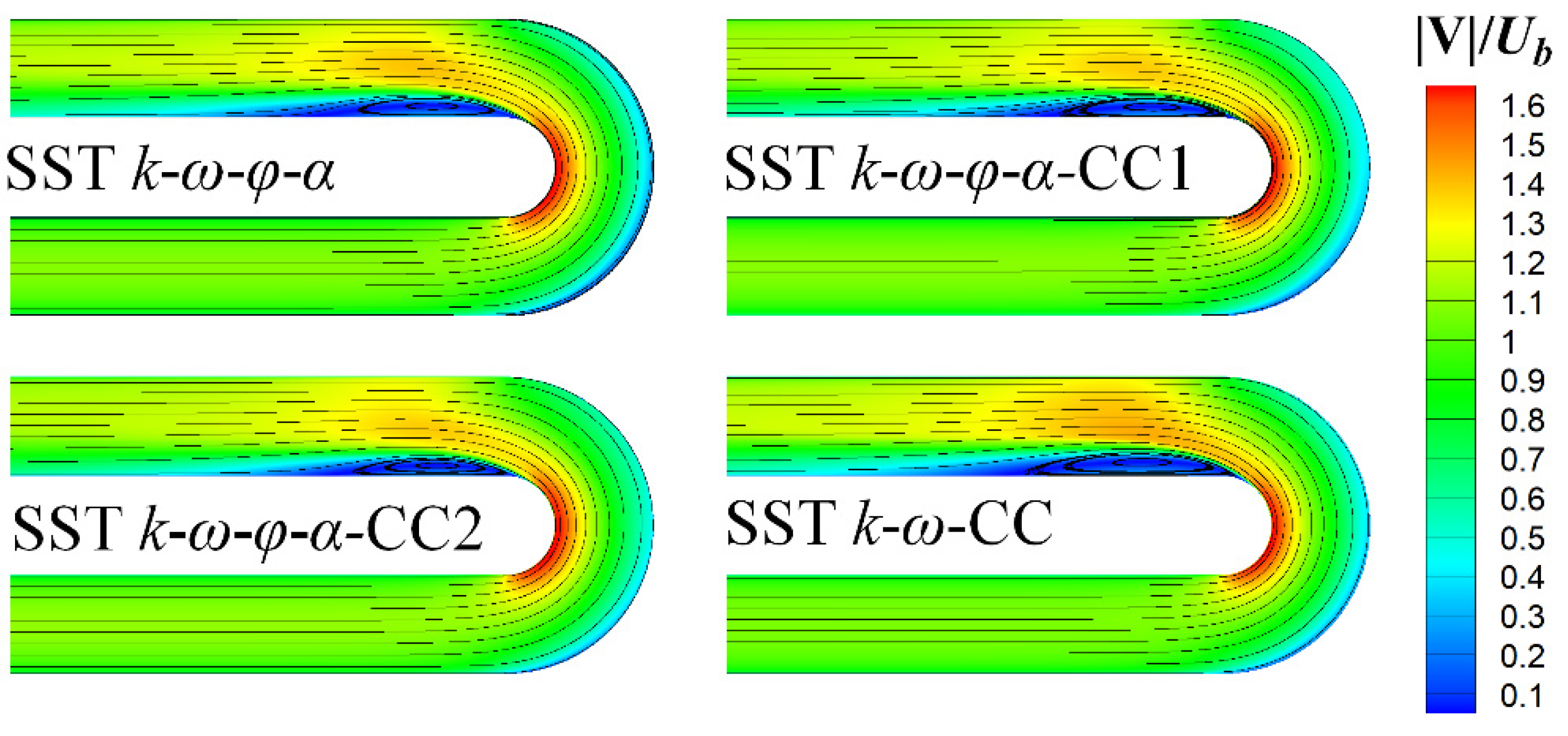
Figure 6 shows the velocity magnitude contours and streamlines predicted by the different turbulence models. Intuitively, the main difference occurred at the flow separation region behind the bend. The separation region predicted by the
model was the largest. Meanwhile, the separation regions predicted by the two proposed models were similar, with both being smaller than that predicted by the original
model.
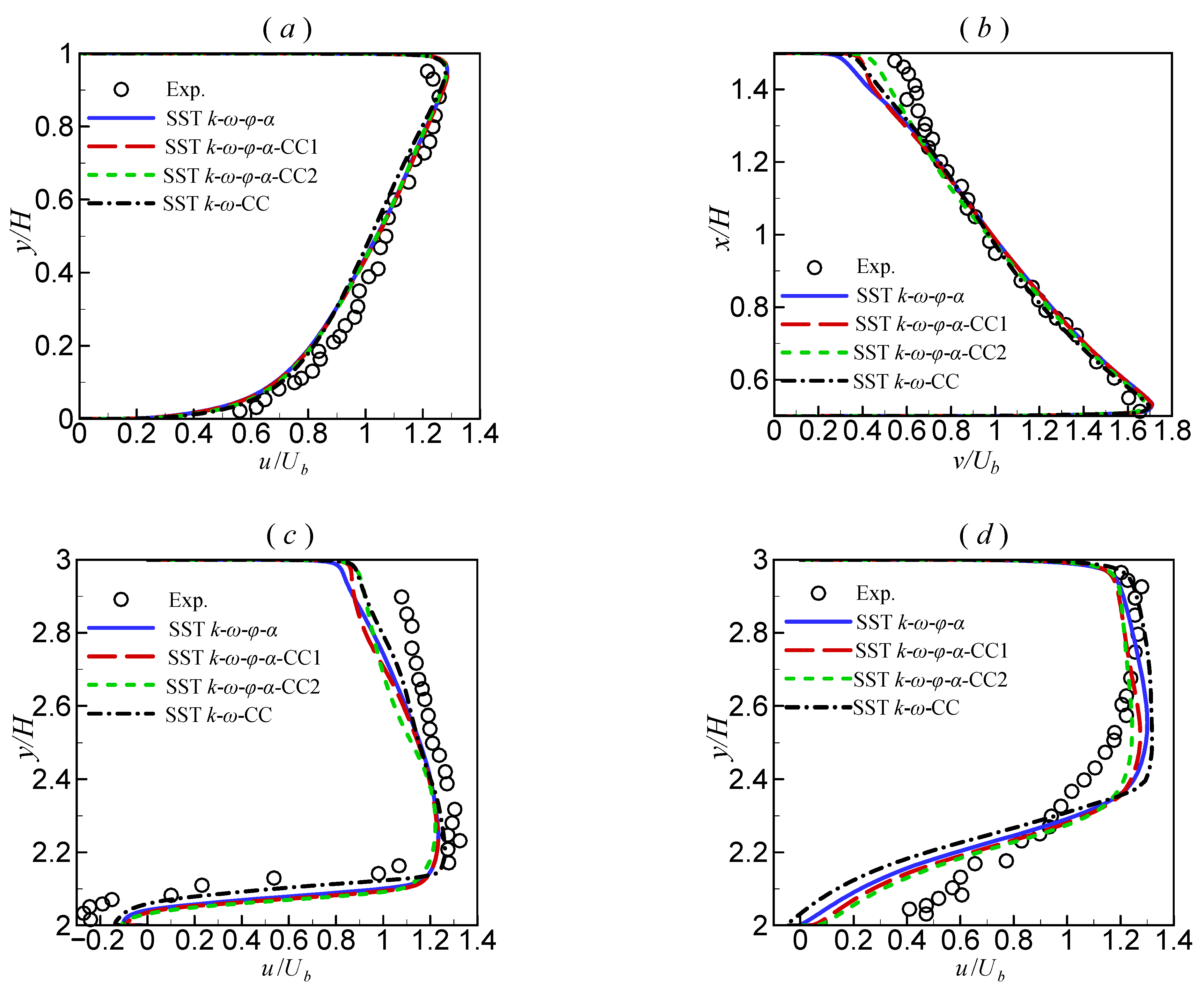
Figure 7 depicts the streamwise velocity profiles along the transverse lines near the bend. To facilitate the analysis, an arc coordinate (s), defined along the center-line of the duct, was used (as shown in
Figure 5). At the beginning of the bend (
,
Figure 7a), the velocity profiles predicted by all turbulence models agreed well with the experimental data. At
, as shown in
Figure 7b, in the region near the outer concave wall, the original
model underpredicted the results. The three other models still underestimated the velocity relative to the experimental results but showed improvements compared to the original
model. At
, as shown in
Figure 7c, the results of all models were not very different. Among them, the velocity predicted by the
model was closer to the experimental data. At
, as shown in
Figure 7d, the
model yielded the worst velocity profile. Moreover, the results predicted by the two proposed models were better than those of the original
model.
Figure 8 shows the turbulent kinetic energy profiles along the transverse lines near the bend. At the locations
and
, both the original
model and the
model suppressed the turbulent kinetic energy near the outer concave wall, while the two proposed models predicted augmentation to varying degrees. Among them, the prediction of the
model was the best. However, although the
model predicted better turbulent kinetic energy, the improvement in velocity prediction was limited. The reason is that this model also predicts higher turbulent dissipation.
The distributions of the friction coefficients (
) along the inner and outer walls are depicted in
Figure 9. The
along the inner wall, predicted by the different turbulence models, varied little. The recovery of
downstream in the re-circulation region is significantly delayed. Along the outer wall, the different turbulence models predicted
differently. The original
model underpredicted while the
model overpredicted the peak of
. The peaks predicted by the two proposed models were similar and agreed well with the experimental data.
Overall, for the 2D U-turn duct flow, the three models with streamline curvature correction provided some improvements. However, it is difficult to determine which performed the best. For example, considering the velocity profile
, the result of the
model was the best; meanwhile, for the velocity profile
, the result of the
model was not good as those of the two proposed models. It should be noted that the results yielded by the
model in this paper were very different from those reported in Smirnov and Menter [
3]. The reasons for this phenomenon may be multi-faceted. For example, the different calculation methods for the second derivative, the different treatment methods for wall boundary conditions, and the different computational platforms. The specific reason should be determined in future research.
3.3. 2D Periodic Hill Flow
The 2D periodic hill flow is also a popular benchmark for assessing turbulence models [
24,
25,
26,
27]. The LES results of Frohlich et al. [
28] have been widely used as a reference. The computational model was constructed based on the LES mentioned above and is illustrated in
Figure 10. The boundary conditions are also shown. The Re (based on the hill height and the bulk velocity at inlet) was 10,595. The total number of mesh cells was 60,800, which was large enough to obtain a grid-independent solution. At the inlet and outlet, a periodic boundary condition was applied. The mass flow rate was specified according to the requirement of Re.
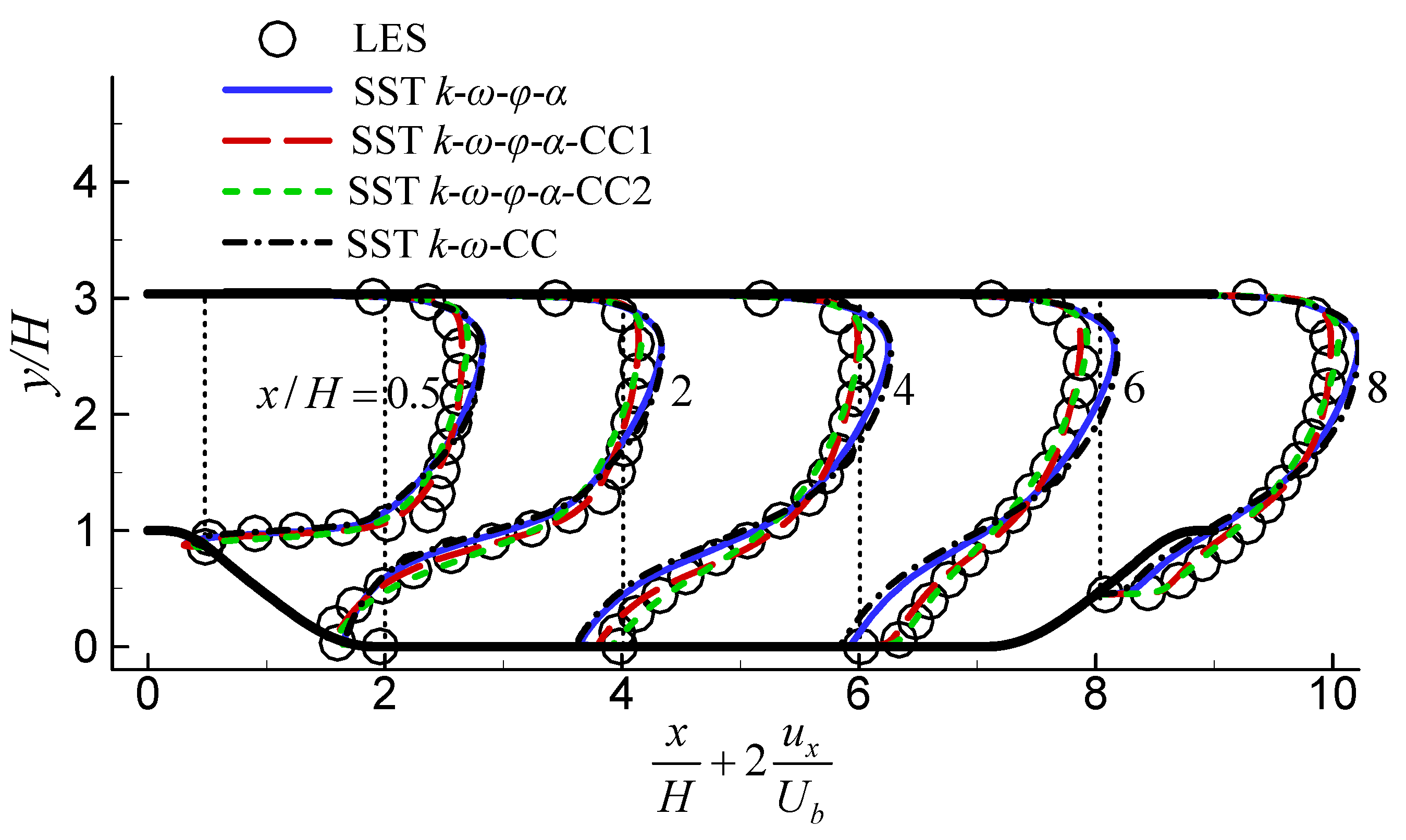
The velocity magnitude contours and streamlines predicted by the different turbulence models are presented in
Figure 11, while the x-direction velocity profiles at different transverse lines are shown in
Figure 12. It is easy to see that both the original
model and the
model predicted excessively large re-circulation zones, while the two proposed models significantly reduced the re-circulation zones. Notably, the
model yielded the smallest re-circulation zone. The velocity profiles obtained with the two proposed models agreed excellently with the LES at all locations. The original
model and the
model predicted higher peak velocities due to the larger re-circulation zone.
Figure 13 depicts the friction coefficient (
) along the bottom wall, and
Table 2 lists the locations of the separation point, re-attachment point, and the length of the re-circulation zone. It is evident that the
predicted by the
model was in excellent agreement with the LES data. The
model also yielded good
. The original
model and the
model predicted similar
, which significantly deviated from the LES result. The separation point was predicted by the original
model slightly later, but the re-attachment point was predicted much later, leading to a much larger re-circulation region. Although the two proposed models also predicted the separation point slightly later, they improved the re-attachment point location strongly, leading to an accurately predicted length of the re-circulation region. The separation point yielded by the
model was very close to LES, but the re-attachment point was strongly delayed.
In summary, the model gave the best results for the 2D periodic hill flow, though the also predicted good results. The original model failed to predict the accurate re-circulation zone behind the hill, demonstrating that streamline curvature correction plays an important role. Although streamline curvature correction was introduced into the model, it did not significantly improve the results, indicating that the model is unsuitable for this flow.
4. Conclusions
A previously developed elliptic blending RANS model was improved by introducing streamline curvature correction. Two approaches were adopted, one of which involved modifying the dissipation term in the
ω-equation, while the other modified the turbulent kinetic energy production term based on Gatski and Speziale’s explicit algebraic stress model [
8]. The two proposed models were assessed using three flows with strongly curved surfaces: The 2D infinite serpentine passage flow, the 2D U-turn duct flow, and the 2D periodic hill flow. The predictions were compared with DNS, experimental, and LES results from the literature. The results computed using the original
model and the
model were also provided as reference. The following conclusions were drawn:
(1) In the 2D infinite serpentine passage flow, the two proposed models produced improved results in terms of the velocity, friction coefficient, and re-circulation length, while the results obtained by the model were the best. Notably, the model was not capable of obtaining correct results: its predictions were even worse than those of the original model.
(2) Compared to the original model, the two proposed models and the model all had positive effects on the 2D U-turn duct flow. The velocity, turbulent kinetic energy, and friction were slightly improved.
(3) In the 2D periodic hill flow, the two proposed models significantly improved upon the results of the original model. They effectively shortened the re-circulation zone and predicted the velocity, friction coefficient, and re-circulation zone more accurately. Again, the predictions by the model were poor.
All cases used to assess the performance of the proposed models in the present paper are 2D. Actually, the
model can be used for 3D flows since the Richardson number is generally suited for arbitrary 3D flows. However, the situation is different for the
model. The regularized anisotropy tensor used (Equation (7)) is only valid for 2D flows, which would cause the model to only work well with 2D flows. Fortunately, an anisotropy tensor suited for 3D flows had been derived [
29]. Although this 3D anisotropy tensor is complex, extending the
model to 3D flows becomes possible, which will be investigated in future work.


