Experimental and Numerical Methods for the Evaluation of Sound Radiated by Vibrating Panels Excited by Electromagnetic Shakers in Automotive Applications

Featured Application

Optimization of vibrating panels excited by electrodynamic shakers for automotive industry applications.

Abstract

Numerical simulations are increasingly employed in the automotive industry to optimize the design stage, reduce prototype testing, and shorten the time to market. The aim of the presented research is the development of a fast and reliable method for the prediction of the sound field generated outside a vehicle by vibrating panels under electromagnetic shaker excitation. Despite that multi-physics numerical simulation software already link mechanical vibrations to their acoustic effect, they show a drawback when calculating the exterior sound field produced by a vibrating panel: the presence of a car model to separate front and rear radiations avoiding the acoustic short circuit, and an air volume surrounding it are required, thus increasing the model complexity and calculation time. Both problems can be overcome with the presented methodology: only the mechanical vibration of the panel is solved numerically, and the radiated sound field is then calculated postprocessing, relying on Rayleigh’s integral. At first, the method’s validation is presented through laboratory experiments; then, a real vehicle panel is analyzed. Comparisons between the finite element method (FEM) simulations and experimental measurements showed very good agreement while keeping the calculation time low for both the laboratory and on-vehicle tests.

1. Introduction

Nowadays, the automotive industry really cares about the sound quality of car cabins. On the one hand, customers demand quieter interiors; on the other hand, hybrid and full electric vehicles, being very silent, are causing inconveniences and danger in urban circulation, as well as unfamiliar feeling in the drivers (especially in the case of sports cars) [1]. Active sound enhancement solutions based on electromagnetic shakers hence find increasing interest. Mostly diffused applications deal with active noise control (ANC) and active vibration control systems [2,3,4,5] for improving the acoustic experience inside or outside the vehicle [6,7,8]. Usually, such systems are mainly effective at low frequencies in the range of 50 Hz–400 Hz for ANC solutions [9,10] or 150 Hz–2 kHz for the Acoustic Vehicle Alerting System (AVAS) [11].

Whatever the application, the positioning of the exciting transducer is critical for maximizing the performance of the system [12]. This requires investigating the vibrational and, consequently, vibroacoustic characteristics of vehicles. Traditionally, it is performed through modal analysis and frequency response functions (FRFs), making use of impact hammers and accelerometers [13,14]. Nevertheless, more recent and efficient noncontact methods are available, such as Laser Doppler Vibrometer (LDV) [15,16,17] or Digital Image Correlation (DIC) [18,19]. They can both be adopted to study vibrations, even though usually DIC is mainly used for structural testing and material identification [20]. At the same time, numerical simulations are more and more employed by car producers for improving the design of acoustics systems [21,22], reducing the need for expensive prototypes and avoiding time-consuming measurements. Therefore, simulation and processing methods capable of reducing the calculation time and providing high-accuracy results are strongly demanded. A common problem deals with the separation between the front and back radiation of a panel to avoid the acoustic short circuit effect [23]. In [24], the authors solved the problem by using an “internal sound hard boundary”, accordingly to [25]. However, this solution can be applied only to simple geometries with the boundary lying on a plane similar to a flat plate. This work, instead, deals with a car bonnet, which would require to introduce in the numerical model the whole car, or at least its front part, to accomplish such requirements. In addition, an air volume surrounding the car should be included too as the simulation domain. Considering the typical dimensions of a car, this would result in a huge number of mesh elements, leading to an unacceptable computational time.

In this paper, a fast and reliable mixed approach (numerical and analytical) to predict the exterior sound field radiated by a vibrating panel of a car under stationary forced excitation is presented. To overcome the aforementioned limitations, the proposed solution relies on an implicit FEM simulation only to solve the mechanical vibration of the panel. Then, the radiated sound field is obtained by calculating the Rayleigh’s integral [26] during postprocessing. In a future development, the authors will consider explicit FEM simulations to analyze more advanced effects related to multiple reflection–refraction of the sound waves in the panels [27,28]. An extensive description of the proposed method is presented in Section 2. In Section 3, the results are shown subdivided between laboratory validation (Section 3.1) and on-vehicle tests (Section 3.2). Eventually, conclusions are summarized in Section 4.

2. Materials and Methods

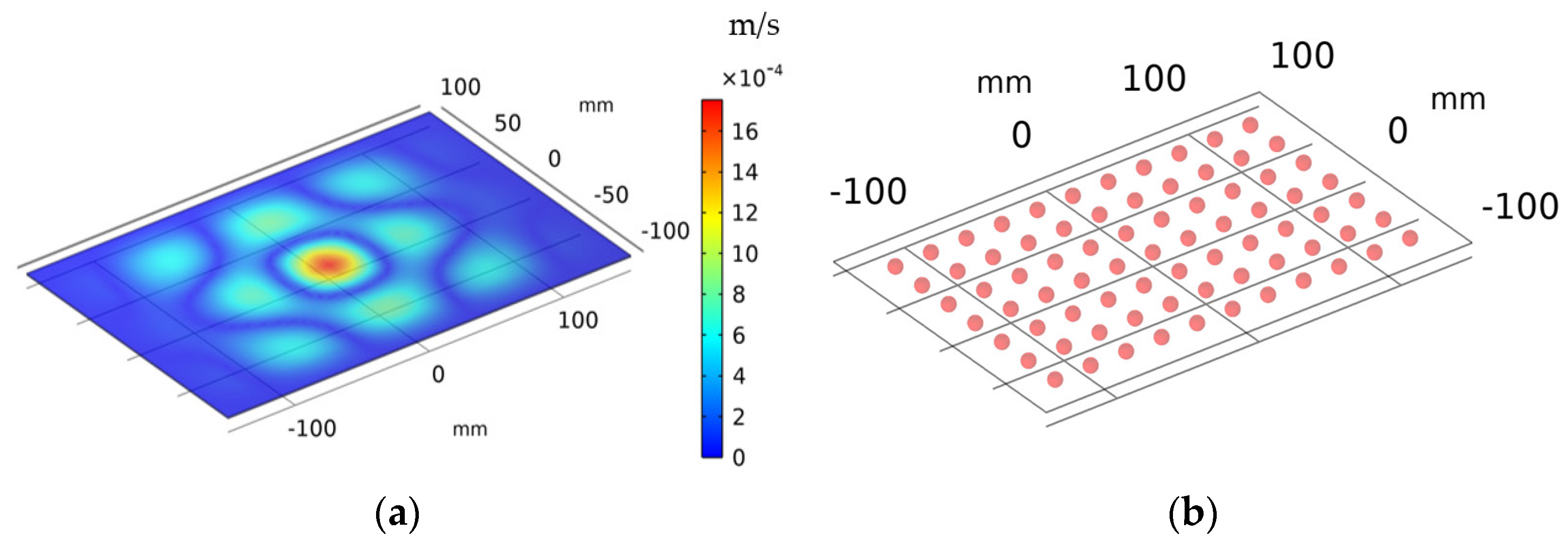
The experimental measurements on the vibrating plate were conducted in the Acoustics Laboratory of the Department of Engineering and Architecture at University of Parma, Italy. The setup was composed of a single-point laser doppler vibrometer by Polytec with processing unit OFV-5000 and sensor head OFV-505. The processing unit is equipped with an analog velocity decoder type VD-01, which was set to provide a measurement range of 25 mm/s/V, with a full-scale output peak of 0.25 m/s (at the maximum output voltage of 10 $V_{peak}$). In this configuration, the maximum frequency was limited to 50 kHz, and a built-in low-pass filter at 20 kHz was activated.

The sensor head was moved by a two-axis handling system with stepping motors (Figure 1a) controlled via laptop computer through an ethernet connection and a dedicated electronic board. The mechanical crosstalk, which is the vibration transmitted to the laser sensor head through the solid path (ground, table, and handling system), was previously evaluated [29], showing a minimum attenuation of −55 dB below 1 kHz, therefore ensuring a satisfactory structural decoupling between the support and the measurement system. An aluminum plate of 300 mm by 200 mm and a thickness of 0.8 mm was positioned below the laser’s sensor head, fixed on a plywood structure (baffle) to separate the front and the back radiation (Figure 1b), as Rayleigh’s integral hypothesis requires [30,31].

A Bruel&Kjaer (B&K) shaker type 4810 was used to excite the plate, and a load cell PCB 208C02 with 11,241 mV/kN sensitivity was screwed on it. The shaker was placed under the plate, rigidly connected to it by a stinger (Figure 2a). With the aim of replicating the experimental setup in the numerical model as closely as possible, the shaker was positioned at the center of the panel.

A reference acoustic measurement of the plate was acquired too by positioning a B&K microphone type 4188 with preamplifier type 2186 above the plate, on-axis with respect to its center, at the standard distance of 1 m (Figure 2b). The Impulse Response (IR) was cut in the time domain for excluding the reflections of the environment (virtual anechoic room technique). The B&K microphone was calibrated with a B&K calibration system type 4231, which produces a pure tone at 1 kHz, having an RMS value of 1 Pa (a SPL of 94 dB re 20 μPa). Such measurement was used for comparing with the SPL reconstructed through Rayleigh’s integral.

Since the OFV-5000 laser controller was not provided with an analog or digital output for delivering the test signal to the amplifier of the shaker, a ZOOM F8 audio interface was employed to manage all input and output signals synchronously (Figure 3). It was connected to the PC via USB and operating at a sampling frequency of 48 kHz. The test signal was an Exponential Sine Sweep (ESS) [32] of 10 s played through the first output channel. The signal was amplified before feeding the shaker at a voltage of 1 Volt, measured with a true-RMS meter. While playing the ESS, three input signals were recorded by the soundcard: force from the load cell, sound pressure from a B&K measurement microphone and velocity from the LDV. Considering the target application, the frequency range of interest was comprised between 150 Hz and 1 kHz. Therefore, an ESS from 20 Hz to 2 kHz was employed for accounting a smooth fade-in and fade-out of 0.5 s, respectively.

The acquisition system was fully calibrated before performing the measurements, so that the results could be directly compared with the simulations. The rated calibration value of 11.2 mV/N was employed for the load cell. A B&K calibration system for accelerometers type 4294 was placed under the sensor head and measured for 20 s to calibrate the laser. It produces a pure tone at 159.2 Hz with a velocity of 10 mm/s (140 dB re 1 nm/s). For the shaker calibration, a pure tone at 159.2 Hz was played through it at 1 V, and a 20-s recording of the vibrating plate was taken with the laser.

A MATLAB code was employed for generating the scanning grid and performing the whole measurement. A regular squared grid with a resolution of 30 mm was created, resulting in a total number of N = 77 points for a measurement time of 20′ (5 s of stabilization delay were employed after every movement of the sensor head).

The FEM model of the rectangular plate was solved in COMSOL Multiphysics, employing shell elements and a quad mesh with the same size of the scanning grid (Figure 4) for a total number of elements equal to 96 and N = 77 nodes. The solution was calculated with a frequency resolution of 1 Hz in the whole frequency range of interest, which was 150 Hz–1 kHz, for a total calculation time of 2′15″. The excitation was a unit force of 1 N applied vertically in the center of the plate (same position of the experimental measurements). The condition of a fully clamped plate was imposed on the edges. COMSOL built-in material properties were used for aluminum: $E=70 \mathrm{GPa}$, $\nu =0.33$, $\rho =2700\mathrm{kg}/{\mathrm{m}}^3$. Damping was introduced as an isotropic loss factor of value $\eta =0.015$, manually tuned against measurements.

The numerical solution is evaluated in all the nodes of the mesh, thus allowing to obtain an output matrix having dimensions (N × K) where N = 77 is the number of nodes and K = 851 is the number of simulated frequencies. The velocity data v was exported to have compatible inputs with the measured data. The velocity will be introduced in Equation (2) for solving the Rayleigh’s integral. In Figure 5a, a surface plot of the velocity magnitude on the plate at 1 kHz can be seen, while, in Figure 5b, a grid of N = 77 points is shown where the solution is evaluated. It must be noted that directly calculating the SPL in COMSOL Multiphysics at the standard distance of 1 m would require a spherical air volume model around the plate, as in [24]. This would have led to a number of elements equal to 226,120 (instead of 96) due to the tetrahedral mesh of the air domain, and a calculation time of 1 h 20′ (instead of 2′15″).

The experimental measurements on a real vehicle panel were carried out at McLaren Automotive facilities. Two measurement sets were taken, with a mini-shaker mounted on the aluminum bonnet of a vehicle in two different positions. During the first measurement, the car hood was subdivided into a regular squared grid made of N = 368 nodes with 50-mm resolution (Figure 6a). The shaker was positioned in the bottom-left corner (Figure 7a), while four monoaxial piezoelectric accelerometers, having a sensitivity of 100 mV/g, were positioned in the nodes of the “mesh”, four at a time (Figure 7b). This provided the acceleration data that will be employed to solve the Rayleigh’s integral with Equation (4). The system was driven by the same Zoom F8 soundcard and amplifier previously described for the laboratory experiment, and the same ESS of 10 s was employed. In addition, a B&K microphone was positioned at the standard distance of 1 m, on-axis with respect to the center of the bonnet. The aim of this first test was providing an experimental verification of the method in a real case, comparing the sound pressure with its estimation based on the Rayleigh integral and experimentally measured data.

In the second measurement, the shaker was positioned in the center of the bonnet (Figure 6b). The panel was excited with the same equipment, but only the B&K microphone was recorded, positioned at the standard distance of 1 m, on-axis with respect to the center. The panel was simulated numerically with the shaker in the same center position for obtaining the acceleration in a grid of points and then reconstructing the sound pressure at the virtual microphone position using the Rayleigh integral (Equation (4)). The aim of this second test was to compare the measured acoustic response of the panel with the numerically simulated result.

The FEM model of the bonnet was solved in COMSOL Multiphysics (Figure 8) in the frequency range 150 Hz–1 kHz with a frequency resolution of 2 Hz. The three-dimensional geometry was simplified to two layers, modeled with shell elements having same thickness of the real panels, which was 0.9 mm for the inferior layer and 1.1 mm for the upper one. A triangular mesh was employed, with a minimum size defined as:

$$mesh\_siz{e}_{min}=c_0/\left(6·f_{max}\right)$$

(1)

where $c_0=343 \mathrm{m}/\mathrm{s}$ is the speed of sound in air at 20 °C, $f_{max}=1 \mathrm{kHz}$ is the maximum interested frequency and factor 6 represents the number of elements per wavelength, where a minimum number of 5 was suggested in [25]. The total number of elements of the mesh was 35,250, for a total simulation time of 1 h 30′. The excitation was a unit force of 1 N applied vertically in correspondence to the red dot visible in Figure 8a. It corresponded to the same position of the shaker on the panel in the second experimental measurements (Figure 6b). The constraints were applied to the edges of the bottom layer (blue dots in Figure 8b) in the corresponding positions of the hinges of the real vehicle. The material properties provided by the car manufacturer were: $E=69 \mathrm{Gpa}$, $\nu =0.33$, $\rho =2710 \mathrm{kg}/{\mathrm{m}}^3$. Additionally, in this case, an isotropic loss factor $\eta =0.015$ was used for damping.

As previously described for the plate, the numerical solution was evaluated in the same nodes of the measurement grid, thus allowing to obtain an output matrix with dimensions (N × K), where N = 368 is the number of nodes and K = 426 is the number of simulated frequencies. The acceleration data a were exported, being compatible with the measured data. The acceleration was employed in Equation (4) for solving Rayleigh’s integral. In Figure 9a, a surface plot of the velocity magnitude on the bonnet at 1 kHz can be seen, while, in Figure 9b, the grid of N = 368 points is shown where the solution is evaluated. It this case, a direct calculation of the SPL in COMSOL Multiphysics at the standard distance of 1 m would have led to a number of elements of about 830,000 (instead of 35,250), considering a spherical air volume around the bonnet, for an estimated calculation time of about 32 h (instead of 1 h 30′). Moreover, this evaluation is strongly underestimated, since the whole car cockpit (or at least the front part of it) should be included in the model, according to the previous explanation, further increasing the number of elements and, thus, the calculation time.

3. Results

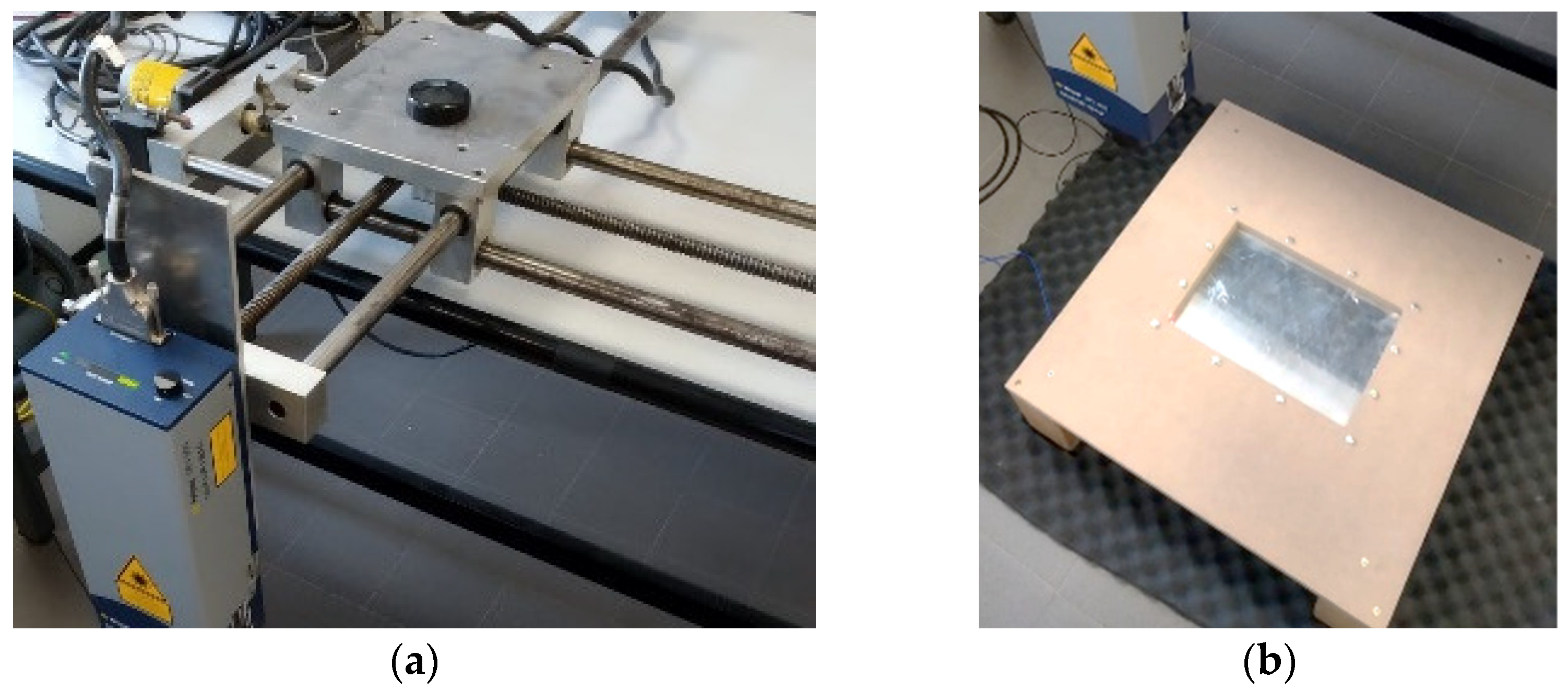
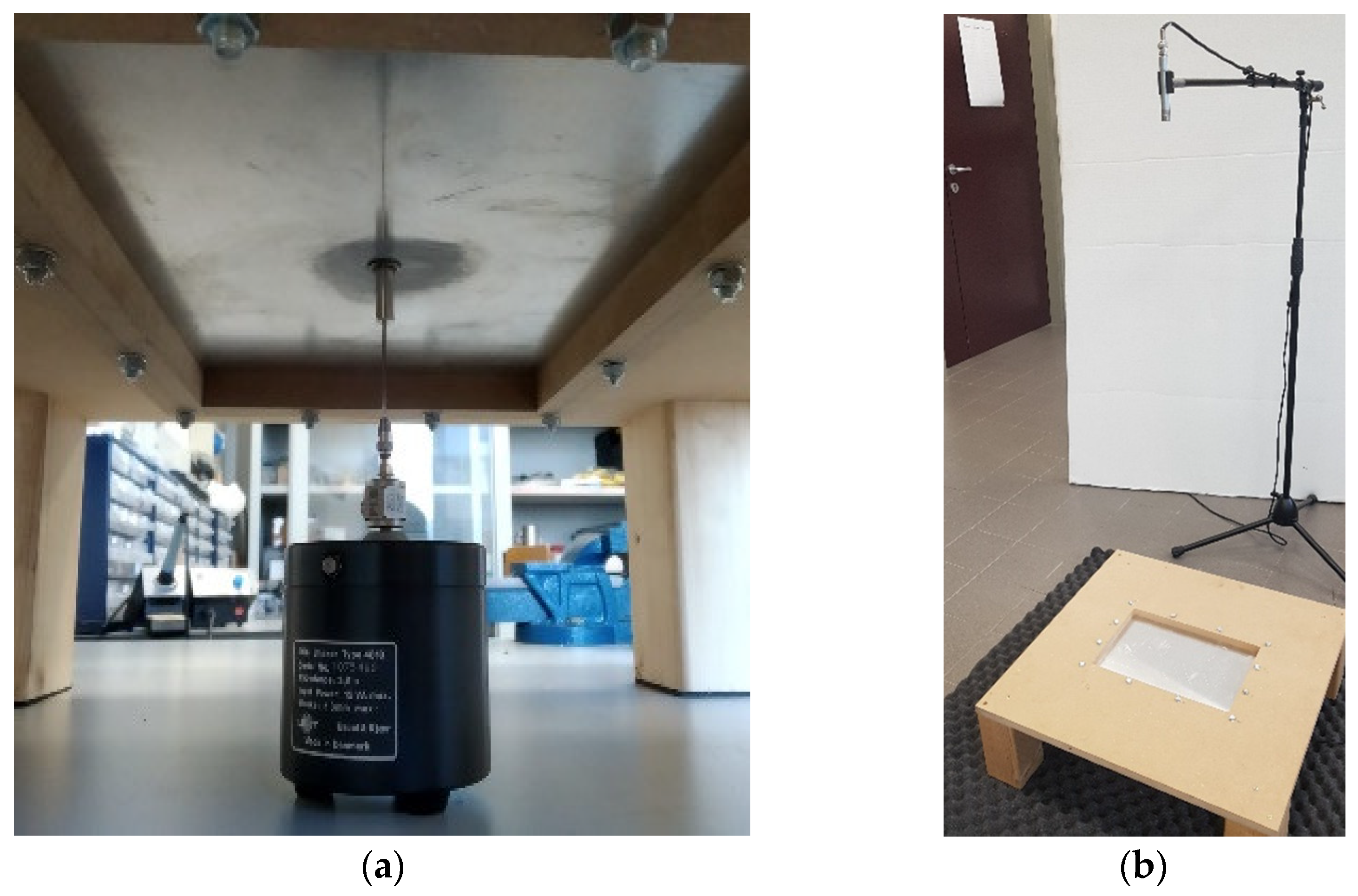
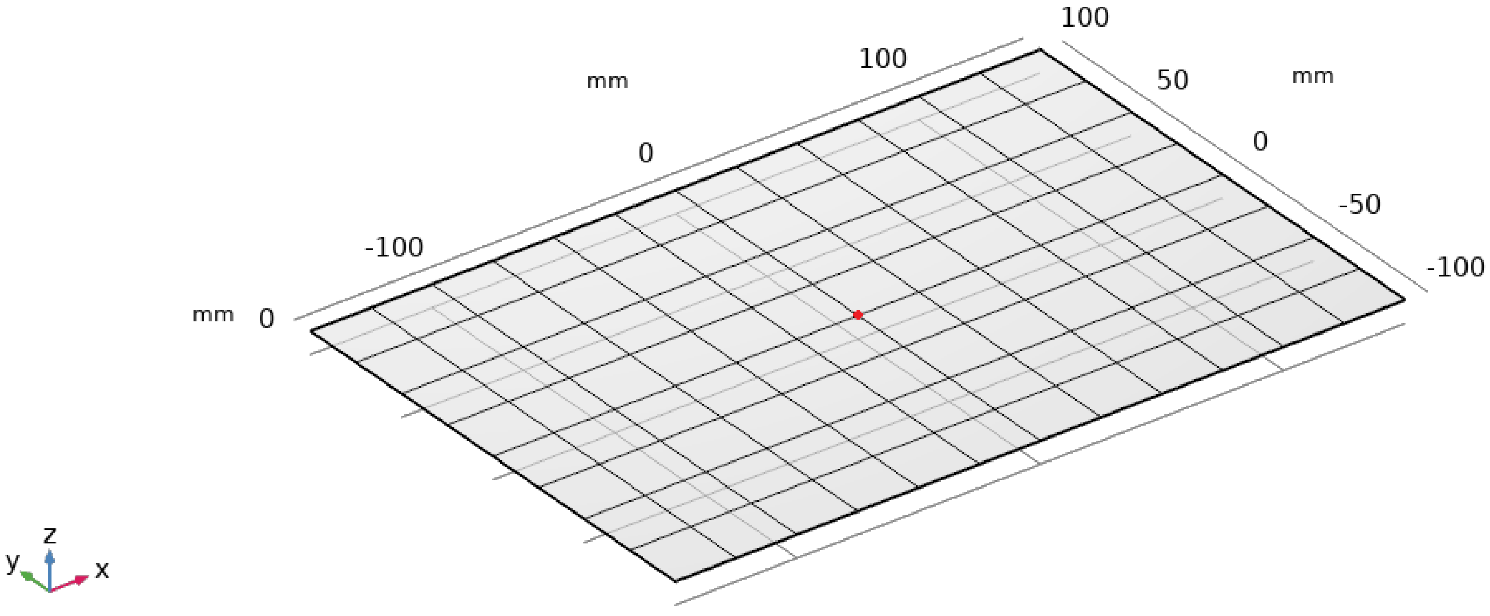
3.1. Laboratory Measurements

At first, the microphone measurement was processed by means of the convolution between the recorded ESS and inverse ESS, thus obtaining the time domain Impulse Response (IR) of the system. The linear part of the IR was cut in the time domain before the first reflection of the environment and converted to the frequency domain by applying Fast Fourier Transform (FFT). Doing so, the spectrum of the sound pressure was obtained for the acoustics reference measurement performed with the B&K microphone on-axis at a distance of 1 m. By applying an equivalent processing, the velocity spectrum in each of the N = 77 points measured by the LDV was obtained too. Then, both the numerical solution and experimental measurement were processed to reconstruct the sound pressure at the microphone position by applying Rayleigh’s integral with the formulation for the velocity data:

$$p\left(r_2,f\right)=\frac{j\omega {\rho }_0}{2\pi }{\displaystyle \sum }_{n=1}^{N}v{\left(r_n, k\right)}_{ }\frac{e^{-i·k·d}}{d}\Delta S_n$$

(2)

where $d$ is the distance between the observing point ($r_2$) and vibrating point ($r_{\mathrm{n}}$), $\rho =1.2 \mathrm{kg}/{\mathrm{m}}^3$ is the air density, ω is the angular frequency, v is the mobility datum, f is the frequency, n is the node index, $\Delta S_n$ is the area of each element and k is the frequency index. In the case of a numerical solution, one can note that v is directly obtained in the frequency domain, therefore making the FFT unnecessary.

In all the three cases, the SPL curve is obtained with the standard conversion formula:

$$SPL\left(f\right)=20·{\log }_{10}\left(\frac{p\left(f\right)}{p_0}\right)$$

(3)

where f is the frequency, p is the sound pressure, and $p_0=20 \mathsf{\mu }\mathrm{Pa}$ is the standard reference value for the sound pressure level. The three results (acoustic measurement with B&K microphone, Rayleigh’s integral applied over measured and numerical data) are compared in Figure 10. One can note a good superimposition of the curves, particularly above 300 Hz. At very low frequencies, below 200 Hz, one can note a turnaround of the microphone peaks with the laser evaluated ones. This is caused by the effect of the IR cut in the time domain before the first reflection, which makes the IR too short to have sufficient information at the lower frequencies. The spectrum obtained by processing numerically calculated data does not present the peak at 550 Hz, which is caused by the nonideality of the experimental setup.

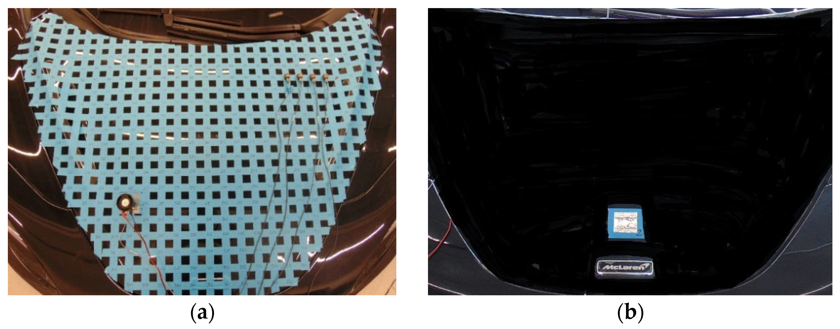
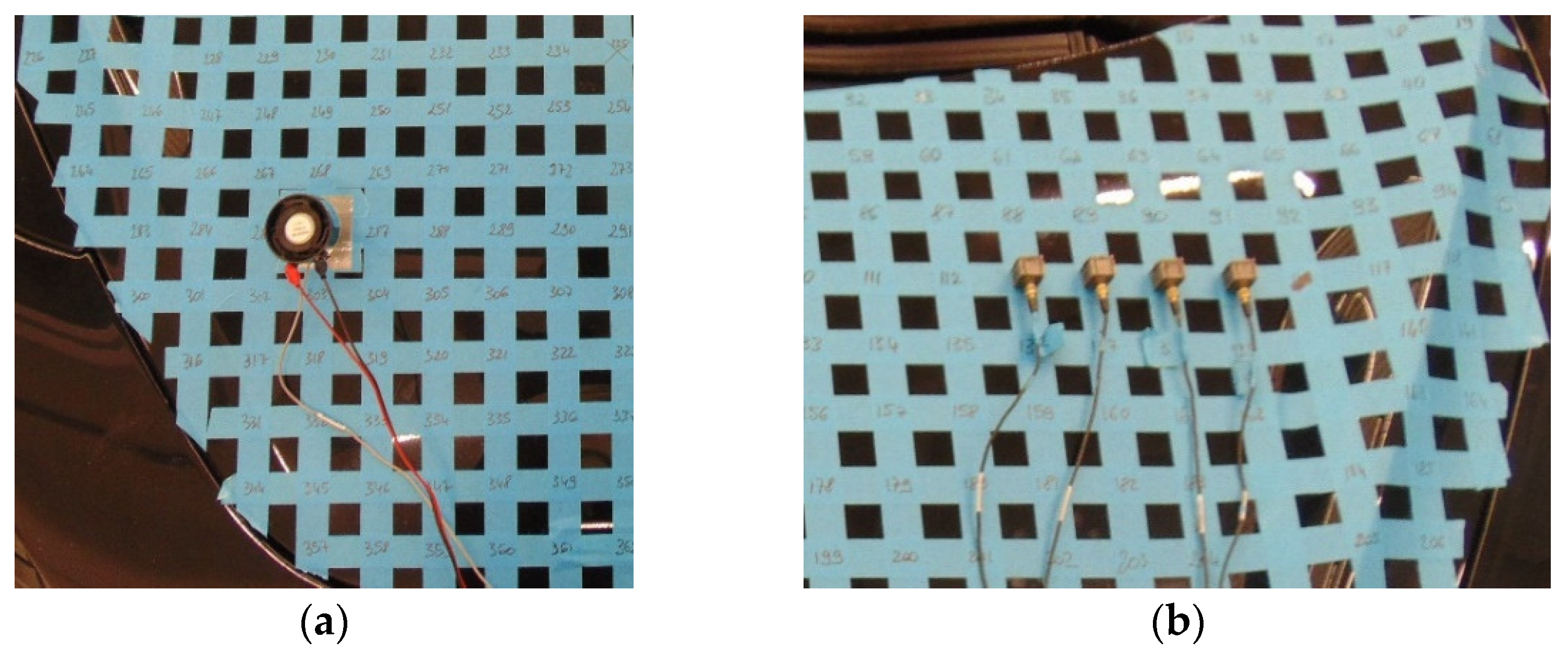
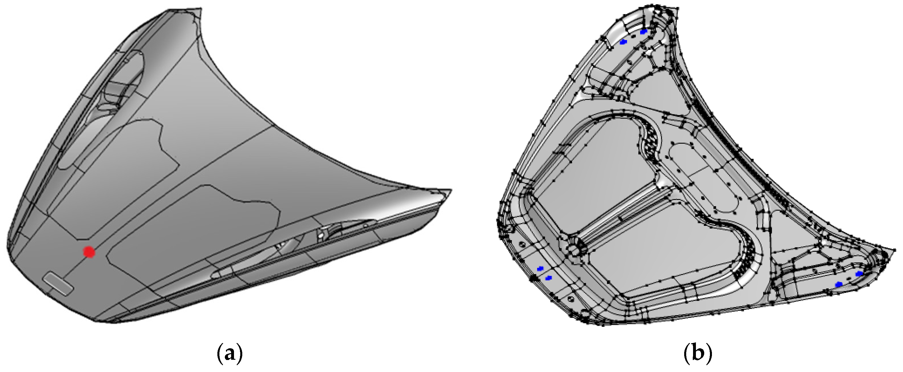
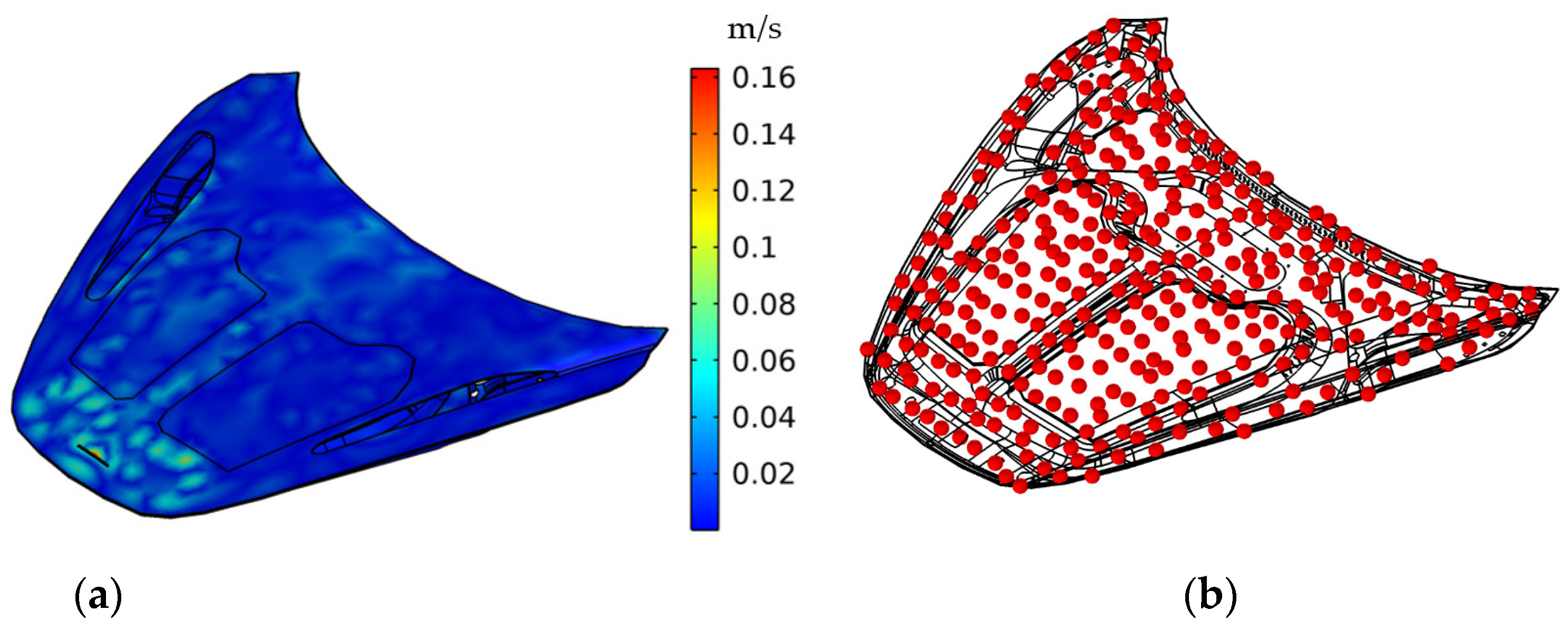
3.2. Vehicle Panel Measurements

The previously described processing (convolution, selection of the linear IRs and FFT) was applied on data measured on the existing vehicle panel, thus obtaining the spectrum of sound pressure measured by the B&K microphone positioned on-axis at a distance of 1 m and the spectrum of acceleration in each of the N = 368 points measured with the four monoaxial accelerometers. Then, both the experimental measurement (Figure 6a) and the numerical solution of the model (Figure 8) were processed to reconstruct the sound pressure at the microphone position by applying the Rayleigh’s integral, with the formulation for the acceleration data:

$$p\left(r_2,f\right)=\frac{{\rho }_0}{2\pi }{\displaystyle \sum }_{n=1}^{N}a{\left(r_n,k\right)}_{ }\frac{e^{-i·k·d}}{d}\Delta S_n$$

(4)

where $d$ is the distance between observing point ($r_2$) and vibrating point ($r_{\mathrm{n}}$), $\rho =1.2 \mathrm{kg}/{\mathrm{m}}^3$ is the air density, a is the acceleration, n is the node index, $\Delta S_n$ is the area of each element and k is the frequency index. In the case of a numerical solution, one can note that a is directly obtained in the frequency domain, therefore making the FFT unnecessary. SPL curves are then obtained with Equation (3). In Figure 11, the microphone recording at a distance of 1 m on-axis is superimposed onto the calculated SPL for the measurement case in Figure 6a. It is visible how, despite some small frequency shifts, the curves’ trends are in good accordance in the whole frequency range of interest. No effect of the IR cut in the time domain can be seen in this case, since the acoustic measurements were performed in the free field, thus allowing to keep the IR longer.

In Figure 12, eventually, the SPL curve reconstructed from the numerical simulation of the vehicle panel (Figure 8) is compared with the recorded SPL at a distance of 1 m (Figure 6b). In this case too, a very good matching between the output of Rayleigh’s integral and the acoustic recording was obtained in the whole frequency range, thus validating the developed approach.

4. Conclusions

A fast and reliable method for predicting the exterior sound field generated by vehicle panels excited with electrodynamic shakers in a steady state was presented. It made use of a mechanical simulation of a single panel vibration and the solution of Rayleigh’s integral over a grid of points where the numerical solution was previously evaluated.

At first, the technique was demonstrated in laboratory conditions by using a flat, aluminum plate fully clamped in a wooden baffle. A mechanical measurement with a LDV, an acoustic measurement with a microphone and a numerical FEM simulation were compared. Then, a real vehicle panel was employed, replacing the LDV with manually moved piezoelectric accelerometers. In both the laboratory and on-vehicle tests, a very good agreement was found between the experimental measurements and numerical solutions.

The presented method allowed for calculating the numerical solution of the vibration on a single panel without including the car geometry for separating the front radiation from the rear radiation or the surrounding air volume, which would be necessary as the solution domain. In this way, it was possible to exclude the undesired effect of an acoustic short-circuit and, at the same time, reducing considerably the complexity of the model and the calculation time.

References

1. Misdariis, N.; Pardo, L.-F. The Sound of Silence of Electric Vehicles—Issues and Answers. In Proceedings of the InterNoise, Hong-Kong, China, 27–30 August 2017. [Google Scholar]
2. Du, X.; Liao, X.; Fu, Q.; Zong, C. Vibro-Acoustic Analysis of Rectangular Plate-Cavity Parallelepiped Coupling System Embedded with 2D Acoustic Black Holes. Appl. Sci. 2022, 12, 4097. [Google Scholar] [CrossRef]
3. Guo, Z.; Pan, J.; Sheng, M. Vibro-Acoustic Performance of a Sandwich Plate with Periodically Inserted Resonators. Appl. Sci. 2019, 9, 3651. [Google Scholar] [CrossRef] [Green Version]
4. Osterziel, J.; Zenger, F.J.; Becker, S. Sound Radiation of Aerodynamically Excited Flat Plates into Cavities. Appl. Sci. 2017, 7, 1062. [Google Scholar] [CrossRef] [Green Version]
5. De Oliveira, L.P.R.; Varoto, P.S.; Sas, P.; Desmet, W. A State-Space Modeling Approach for Active Structural Acoustic Control. Shock Vib. 2009, 16, 797125. [Google Scholar] [CrossRef]
6. Roberts, M.; Grieco, J.; Ellis, C. Diffuse-field Radiators in Automotive Sound System Design. In Proceedings of the 108th Audio Engineering Society Convention, Paris, France, 19–22 February 2000; p. 5163. [Google Scholar]
7. Dhandole, S.; Modak, S.V. Review of vibro-acoustics analysis procedures for prediction of low frequency noise inside a cavity. In Proceedings of the 25th Conference & Exposition on Structural Dynamics, Orlando, FL, USA, 19–22 February 2007. [Google Scholar]
8. Ma, X.; Wang, L.; Xu, J. Active Vibration Control of Rib Stiffened Plate by Using Decentralized Velocity Feedback Controllers with Inertial Actuators. Appl. Sci. 2019, 9, 3188. [Google Scholar] [CrossRef] [Green Version]
9. Belicchi, C.; Opinto, A.; Martalo, M.; Tira, A.; Pinardi, D.; Farina, A.; Ferrari, G. ANC: A low-cost implementation perspective. In Proceedings of the 12th International Styrian Noise, Vibration & Harshness Congress: The European Automotive Noise Conference, Graz, Austria, 22–24 June 2022. [Google Scholar] [CrossRef]
10. Tripodi, C.; Costalunga, A.; Ebri, L.; Vizzaccaro, M.; Cattani, L.; Ugolotti, E.; Nili, T. Experimental Results on Active Road Noise Cancellation in Car Interior. In Proceedings of the 144th Audio Engineering Society Convention, Milan, Italy, 23–26 May 2018; p. 9976. [Google Scholar]
11. Tsuruta-Hamamura, M.; Kobayashi, T.; Kosuge, T.; Hasegawa, H. The Effect of a ‘Design-of-Awareness’ Process on Recognition of AVAS Sound of Quiet Vehicles. Appl. Sci. 2022, 12, 157. [Google Scholar] [CrossRef]
12. Chatterjee, A.; Ranjan, V.; Azam, M.S.; Rao, M. Comparison for the Effect of Different Attachment of Point Masses on Vibroacoustic Behavior of Parabolic Tapered Annular Circular Plate. Appl. Sci. 2019, 9, 745. [Google Scholar] [CrossRef] [Green Version]
13. Anerao, N.; Kumar, T. Vibro-Acoustic Reciprocity Analysis Using Dodecahedral Sound Source and Its Application for Material Assessment. 2020. Available online: https://www.researchgate.net/profile/Nitesh-Anerao/publication/349830062_Vibro-Acoustic_reciprocity_analysis_using_dodecahedral_sound_source_and_it’s_application_for_material_assessment/links/60427d114585154e8c78a0fa/Vibro-Acoustic-reciprocity-analysis-using-dodecahedral-sound-source-and-its-application-for-material-assessment.pdf (accessed on 5 March 2021).
14. Dowsett, A.; O’Boy, D.; Walsh, S.; Abolfathi, A.; Fisher, S. The prediction of measurement variability in an automotive application by the use of a coherence formulation. Proc. Inst. Mech. Eng. Pt. D J. Automob. Eng. 2018, 232, 1694–1700. [Google Scholar] [CrossRef]
15. Scislo, L. Quality Assurance and Control of Steel Blade Production Using Full Non-Contact Frequency Response Analysis and 3D Laser Doppler Scanning Vibrometry System. In Proceedings of the 2021 11th IEEE International Conference on Intelligent Data Acquisition and Advanced Computing Systems: Technology and Applications (IDAACS), Cracow, Poland, 22–25 September 2021; Volume 1, pp. 419–423. [Google Scholar] [CrossRef]
16. Scislo, L.; Guinchard, M. Non-invasive Measurements of Ultra-Lightweight Composite Materials using Laser Doppler Vibrometry System. In Proceedings of the 26th International Congress on Sound and Vibration, Montreal bridges, QC, Canada, 7–11 July 2019; Available online: https://www.researchgate.net/publication/358090716_Non-invasive_measurements_of_ultra-lightweight_composite_materials_using_Laser_Doppler_Vibrometry_system (accessed on 25 January 2022).
17. Collini, L.; Farina, A.; Garziera, R.; Pinardi, D.; Riabova, K. Application of laser vibrometer for the study of loudspeaker dynamics. Mater. Today Proc. 2017, 4, 5773–5778. [Google Scholar] [CrossRef]
18. Molina-Viedma, Á.; López-Alba, E.; Felipe-Sesé, L.; Díaz, F.; Rodríguez-Ahlquist, J.; Iglesias-Vallejo, M. Modal Parameters Evaluation in a Full-Scale Aircraft Demonstrator under Different Environmental Conditions Using HS 3D-DIC. Materials 2018, 11, 230. [Google Scholar] [CrossRef] [PubMed] [Green Version]
19. Seguel, F.; Meruane, V. Damage assessment in a sandwich panel based on full-field vibration measurements. J. Sound Vib. 2018, 417, 1–18. [Google Scholar] [CrossRef]
20. Di Lorenzo, E.; Mastrodicasa, D.; Wittevrongel, L.; Lava, P.; Peeters, B. Full-Field Modal Analysis by Using Digital Image Correlation Technique. In Rotating Machinery, Optical Methods & Scanning LDV Methods; Springer: Cham, Switzerland, 2020; Volume 6, pp. 119–130. [Google Scholar]
21. Pinardi, D.; Farina, A.; Park, J.-S. Low Frequency Simulations for Ambisonics Auralization of a Car Sound System. In Proceedings of the 2021 Immersive and 3D Audio: From Architecture to Automotive (I3DA), Bologna, Italy, 8–10 September 2021; pp. 1–10. [Google Scholar] [CrossRef]
22. Pinardi, D.; Riabova, K.; Binelli, M.; Farina, A.; Park, J.-S. Geometrical Acoustics Simulations for Ambisonics Auralization of a Car Sound System at High Frequency. In Proceedings of the 2021 Immersive and 3D Audio: From Architecture to Automotive (I3DA), Bologna, Italy, 8–10 September 2021; pp. 1–10. [Google Scholar] [CrossRef]
23. Misak, S.; Pokorny, V.; Kacor, P. Modeling of Acoustic Short Circuits. In Intelligent Data Analysis and Applications; Springer: Cham, Switzerland, 2015; pp. 121–131. [Google Scholar]
24. Tira, A.; Pinardi, D.; Belicchi, C.; Farina, A.; Figuretti, A.; Izzo, S. ANC: A Low-Cost Implementation Perspective. In Proceedings of the 12th International Styrian Noise, Vibration and Harshness Congress: The European Automotive Noise Conference, Graz, Austria, 22–24 June 2022. [Google Scholar] [CrossRef]
25. COMSOL. Acoustics Module User’s Guide. Available online: https://doc.comsol.com/5.4/doc/com.comsol.help.aco/AcousticsModuleUsersGuide.pdf (accessed on 26 October 2022).
26. Leissa, A.W. The historical bases of the Rayleigh and Ritz methods. J. Sound Vib. 2005, 287, 961–978. [Google Scholar] [CrossRef]
27. Kuznetsov, S. SH-waves in laminated plates. Q. Appl. Math. 2006, 64, 153–165. [Google Scholar] [CrossRef]
28. Goldstein, R.V.; Kuznetsov, S.V. Long-Wave Asymptotics of Lamb Waves. Mech. Solids 2017, 52, 700–707. [Google Scholar] [CrossRef]
29. Bellini, M.C.; Collini, L.; Farina, A.; Pinardi, D.; Riabova, K. Measurements of loudspeakers with a laser doppler vibrometer and the exponential sine sweep excitation technique. J. Audio Eng. Soc. 2017, 65, 600–612. [Google Scholar] [CrossRef]
30. Sung, C.-C.; Jan, C.T. Active control of structurally radiated sound from plates. J. Acoust. Soc. Am. 1997, 102, 370–381. [Google Scholar] [CrossRef]
31. Klippel, W.; Schlechter, J. Distributed Mechanical Parameters Describing Vibration and Sound Radiation of Loudspeaker Drive Units. In Proceedings of the 125th Audio Engineering Society Convention, San Francisco, CA, USA, 2–5 October 2008; p. 7531. [Google Scholar]
32. Farina, A. Simultaneous Measurement of Impulse Response and Distortion with a Swept-Sine Technique. In Proceedings of the 108th Audio Engineering Society Convention, Paris, France, 19–22 February 2000; p. 5093. [Google Scholar]
Figure 1. (a) Two-axis handling system of laser sensor head and (b) fully clamped aluminum plate mounted on a rigid baffle.
Applsci 12 11210 g001
Figure 2. (a) B&K shaker type 4810 connected to the plate via a stinger. The PCB load cell is visible at the top of the shaker. (b) Acoustic measurement of the plate with a B&K microphone at 1 m on-axis.
Applsci 12 11210 g002
Figure 3. Block diagram of the experimental measurement setup.
Applsci 12 11210 g003
Figure 4. FEM model of the aluminum plate; the exciting point is highlighted in red.
Applsci 12 11210 g004
Figure 5. (a) Velocity magnitude over the plate at 1 kHz. (b) Grid of N = 77 points where the velocity data are evaluated.
Applsci 12 11210 g005
Figure 6. (a) Test vehicle bonnet subdivided into a grid of N = 368 measurement points. (b) Scheme of second measurement shaker’s position (low center) of the bonnet.
Applsci 12 11210 g006
Figure 7. (a) Details of the test vehicle bonnet, with a mini-shaker on the bottom-left. (b) Details of the test vehicle bonnet with four accelerometers on the top-right.
Applsci 12 11210 g007
Figure 8. (a) View from above of the model of the car’s hood adopted for the numerical vibrational analysis. The red dot indicates the force application point. (b) View from below. The blue dots indicate the constraint application points.
Applsci 12 11210 g008
Figure 9. (a) Velocity magnitude over the bonnet at 1 kHz. (b) Grid of N = 368 points where the velocity data are evaluated on the upper surface of the bonnet.
Applsci 12 11210 g009
Figure 10. SPL recorded by microphone (solid line) superimposed with SPL calculated by Rayleigh’s integral (dash line).
Applsci 12 11210 g010
Figure 11. SPL recorded by a microphone (solid line) superimposed with SPL calculated by Rayleigh’s integral (dash line) from real panel measurements at McLaren Automotive.
Applsci 12 11210 g011
Figure 12. SPL recorded by microphone (solid line) superimposed with SPL calculated by Rayleigh’s integral (dash line) from numerically simulated data.
Applsci 12 11210 g012
Publisher’s Note: MDPI stays neutral with regard to jurisdictional claims in published maps and institutional affiliations.