A New Sensor System for Accurate 3D Surface Measurements and Modeling of Underwater Objects

Featured Application

A potential application of the work is the underwater 3D inspection of industrial structures, such as oil and gas pipelines, offshore wind turbine foundations, or anchor chains.

Abstract

A new underwater 3D scanning device based on structured illumination and designed for continuous capture of object data in motion for deep sea inspection applications is introduced. The sensor permanently captures 3D data of the inspected surface and generates a 3D surface model in real time. Sensor velocities up to 0.7 m/s are directly compensated while capturing camera images for the 3D reconstruction pipeline. The accuracy results of static measurements of special specimens in a water basin with clear water show the high accuracy potential of the scanner in the sub-millimeter range. Measurement examples with a moving sensor show the significance of the proposed motion compensation and the ability to generate a 3D model by merging individual scans. Future application tests in offshore environments will show the practical potential of the sensor for the desired inspection tasks.

1. Introduction

Three-dimensional acquisition of objects underwater is gaining importance in the field of inspection. Industrial facilities, such as offshore wind turbine foundations, oil and gas pipeline systems, underwater structures, and other objects, including anchor chains, are regularly required to be measured underwater [1,2]. Other objects of interest for underwater 3D measurements include archaeological sites on the seabed [3,4,5,6,7], sunken shipwrecks [8], plant and coral growth [9], and the biomass or size of fish populations [10,11,12]. Several contactless methods have been applied to perform 3D reconstruction underwater. Examples includes techniques using sonar systems, laser scanning, time-of-flight (ToF) cameras, and photogrammetry.

Whereas sonar systems [13,14,15,16] provide fast measurements of large areas over long distances, their measurement accuracy is low compared to that of optical sensors.

Mariani et al. introduced a new ToF based system called UTOFIA [17], providing an accuracy of approximately 10 cm at a 14 m distance. A commercially available ToF system is provided by 3D at Depth [18].

Laser scanning systems [1,2,19,20] provide fast acquisition, long ranges, high measurement accuracy, and robustness against water turbidity. Additionally, measurements can be performed in motion. Because line laser scanning systems typically capture only a single or a few 2D profiles at a time, 3D registration and merging of individual consecutive 3D scans is not feasible. Therefore, for 3D mapping purposes, the trajectory is often estimated using visual odometry [21] or vehicle navigation and motion data [22]. However, the resulting measurement accuracy is not comparable to the potential accuracy of photogrammetric measurements. Commercially available laser scanning systems for underwater use are produced by, e.g., CathXOcean [23] and Voyis [24].

However, high-accuracy photogrammetry requires either preparation effort comprising placement of markers, textured objects, or support of structured illumination. Photogrammetric systems have been introduced by Kwon [25], Telem and Filin [26], Sedlazeck and Koch [27], and others [3,5,28,29]. Beall [30] provided a photogrammetric solution for reconstruction of large underwater structures with low accuracy using video streams of a stereo rig. An interesting new approach to underwater 3D measurements was provided by Skinner [31] by using a plenoptic camera.

Structured illumination has been applied for precise underwater measurements in several research projects. It has been shown to be suitable for close distances and small objects. Examples of such systems have been presented by Bruno et al. [32], Bianco et al. [33], and Bräuer-Burchardt et al. [34].

These systems have shown potential regarding high measurement accuracy of this reconstruction technique. However, illumination power of the pattern projectors in these systems are typically too low to satisfy the needs of challenging industrial inspection tasks. Namely, they should have a large field of view, be able to measure along large distances, be able to accommodate the very small amount of time available for scanning and data processing, and, finally, be able to generate 3D surface models of the observed object in real time. In addition to an accurate camera technique, this requires a high illumination power for structured light patterns, a cooling concept for the dissipation of produced heat, and high-power computational equipment for processing the large quantity of data. Modern developments in hardware components, which are necessary to build structured light-based optical 3D scanners, offer hope of overcoming the current restrictions regarding insufficient measurement volume size and measurement distance of such devices for underwater use.

One of the most challenging tasks regarding the use of 3D stereo scanning systems based on structured illumination is the capture of fast-moving objects or the motion of the sensor itself. This is due to the relatively long exposure time necessary for acquisition. A typical temporal sequence length necessary for realization of point correspondence is ten images. Hence, without motion correction, the distance covered in the time needed to record ten images leads to a change or smearing of the projected pattern observed in a given pixel.

Lam et al. [35] introduced a novel motion compensation method for structured light-based scanning systems, where the projection unit actively takes part in 3D point calculation. Other techniques exploit the motion blur of the projected pattern for 3D shape estimation [36].

Recently, low-budget 3D reconstruction and merging was applied to underwater 3D seabed measurement in nearshore shallow waters using video streams of an action sport cam and structure from motion (SfM) technology [37]. Another interesting application of merged 3D point clouds was introduced by Catalucci et al. [38] for boat shape measurement in air using a 3D hand scanner and photo-modeling technique. These new methodologies for 3D model generation with a moving camera or scanner, respectively, were introduced at a workshop on metrology for the sea [39].

Our aim was to investigate the application of a new stereo scanning systems supported by structured illumination for precise, continuous 3D capturing and modeling of underwater structures at medium-range measurement distances (up to 3 m) and fields of view of about 1 m².

In the remainder of this paper, the development of an appropriate 3D sensor system is described; first, results are presented, as well as examples of measurements and the construction of 3D models of the captured objects.

2. Materials and Methods

2.1. New Sensor System

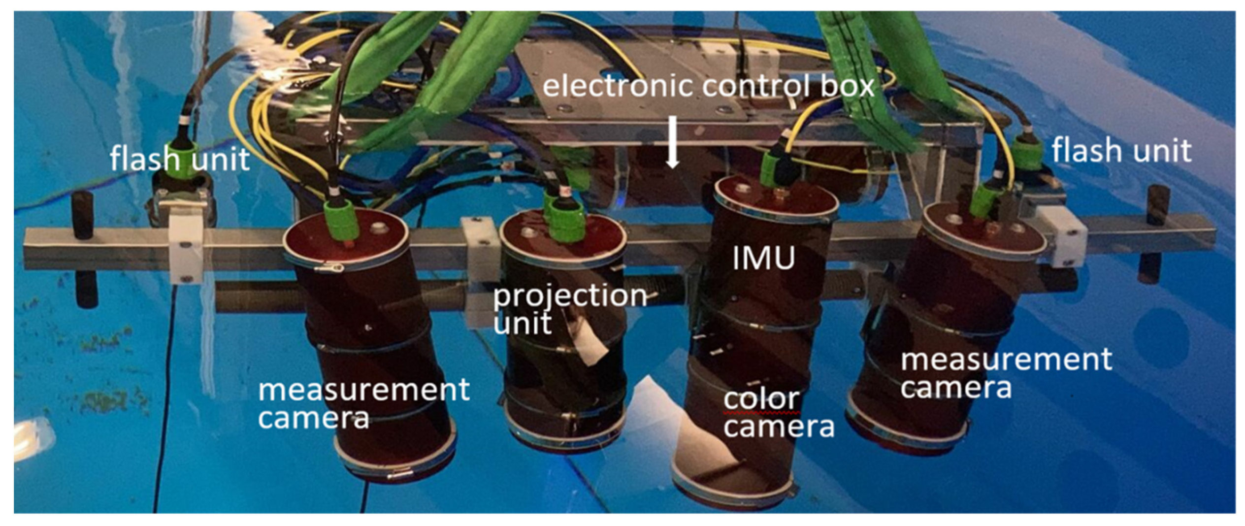
2.1.1. Hardware Setup

We developed a sensor system based on structured light illumination for an underwater 3D inspection system for industrial structures according to the requirements of potential users. Its targeted application is the inspection of oil and gas pipelines, offshore windmill fundaments, anchor chains, and other technical structures. It can be mounted to a remotely operated vehicle (ROV), and it can be controlled remotely from a vessel. It captures up to sixty 3D scans per second with a velocity up to 1 m/s. It has a field of view of about 1 m² and captures 3D data at distances between approximately 1.6 m and 2.4 m. The system was built as a laboratory setup (see Figure 1). The sensor system, called UWS (underwater sensor), was developed according to the requirements within a funded research project (see acknowledgements).

The sensor system consists of:

• Two monochrome measurement cameras arranged in a stereo setup for 3D data acquisition;
• A projection unit producing structured illumination patterns;
• A color camera for navigation and additional visual odometry data capture;
• Two high-power LED flash units, providing synchronized homogenous illumination for the color camera;
• A fiberoptic gyro (FOG) inertial measurement unit (IMU) for motion estimation to support global reconstruction tasks using SLAM algorithms;
• Underwater housings for each camera and the projection unit (IMU is in the housing of the color camera);
• An electronic control and interface box.

An additional necessary piece of equipment is a PC workstation for control and storage of the measurement data and power supply, which can be positioned on the vessel and is connected to the UWS. The cameras and lenses are commercially available parts. The projection unit is a Fraunhofer IOF development consisting mainly of an LED light source, a rotating slide (GOBO wheel) and motor, a projection lens, and control electronics. The projection unit realizes the generation of a structured light pattern in the form of an aperiodic sinusoidal fringe pattern (see [40]).

2.1.2. 3D Data Generation

Measurement data are generated from the stereo camera image stream supported by the aperiodic fringe projection GOBO unit. The common principle of triangulation of corresponding points in the camera images using the calibrated camera geometries is applied (see [41]). We use advanced pinhole modeling, which takes into account the refraction of the vision rays at the interfaces of the different media air, glass, and water.

The corresponding point search is realized using the generation of structured temporal patterns by the GOBO-based projection unit. Typically, ten consecutive images are used to form the temporal pattern of grey values at one pixel. Correspondence is found by choosing the highest correlation value along the epipolar lines (see [40]).

2.1.3. Geometric Modeling

To obtain optimal geometric 3D sensor modeling, an extensive theoretical geometrical analysis of the optical sensor components (cameras, lenses, and glass cover) and the additional important conditions and features was performed.

Furthermore, refraction of the vision rays at the interfaces between air and glass and glass and water has to be considered in the geometric camera modeling. This was done using an extended pinhole model (see [42,43]). Simulations revealed that the systematic measurement error of our stereo system with the actual geometric parameters was weak over the complete measurement distance (2.0 m ± 0.4 m), even if a simple pinhole model including distortion correction was used.

As a result of the camera model analysis, an extended pinhole camera model was selected as a 3D sensor model, leading to minimal systematic measurement errors. A detailed description of the geometric property analysis is given in [43].

2.1.4. Sensor Calibration

One precondition for the 3D measurement process is the calibration of the sensor system. The parts of the UWS to be calibrated are:

• The 3D scanning unit, consisting of two monochrome measurement cameras arranged in a stereo array;
• The color camera (to be calibrated with respect to one of the stereo cameras);
• The IMU (to be calibrated with respect to the color camera).

In the following section, the calibration of the 3D sensor is briefly described. According to the theoretical analysis mentioned in Section 2.1.3, we selected the extended pinhole model with distortion correction function.

Sensor calibration was performed in a water basin using a set of ArUco [44] and circle markers in a plane-near arrangement (see Figure 2). The marker boards were placed on the floor of the basin, and the sensor was positioned in certain orientations according to the scene, using a gantry system. The image data were recorded continuously in video mode. Hence, more data than necessary (from approximately ten different sensor positions) were recorded. Calibration points were selected automatically using our own software tool, and calibration parameters were calculated using the commercially available BINGO bundle adjustment software [45].

Calibration was evaluated using consecutively performed static measurements of given specimens, such as a ball bar and a plane-normal with calibrated measures. After analysis of the evaluation measurements of the ball bar, a 3D error-compensation function was generated and used as the final part of the calibration. Results of the evaluation measurements are documented in Section 3.

Calibration of the color camera was performed analogously using BINGO software, whereas IMU calibration was performed according to the method introduced by Furgale et al. [46].

An extensive survey of different calibration procedures of underwater systems was conducted by Shortis [47].

2.2. Data Recording in Movement

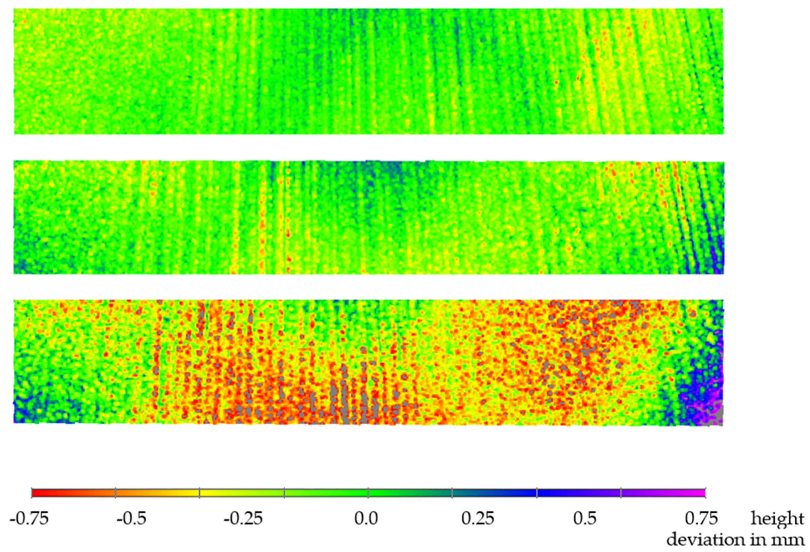
2.2.1. Effects of Sensor Movement on Measurement Data

The relative movement between recording camera and observed measurement object leads to a shift of the pixels representing a given object point. When this shift exceeds one or two pixels per sequence recording, it leads to smearing of the image points comparable to the application of an average filter operator. Therefore, it leads to errors in 3D measurement.

If these errors are to be corrected, the typical application scenarios of the sensor must be considered. Let us consider the case of a linear sensor motion with constant velocity v, image sequence length n, and 2D image frame rate f. For simplicity and due to the lack of exact a priori information concerning the object distance of a mapped point, we assume a constant object distance, d. Additionally, the virtual principal distance, c, the pixel size, ps, and the binning factor, b, are influencing parameters. The pixel shift, Δs (in camera pixels), is:

Δs = v · c · n/(f · d · b · ps).

(1)

Let us consider the case of fast sensor motion and high 2D image frame rate f. Let v = 1 m/s, c = 17 mm, ps = 0.009 mm (binning mode), d = 2 m, and f = 900 Hz. Additionally, we assume a motion direction mainly in the Y direction of the camera coordinate system (perpendicular to the optical axis of the system). Let us consider a ten-image (n = 10) sequence recording to obtain one 3D scan. The image recording time is approximately 10/900 Hz ≈ 11 ms. The actual movement, ΔS, of the sensor in this time is 11 mm. An object point at a 2 m distance “moves” in the image plane Δs ≈ 10.4 px per sequence, i.e., approximately one pixel per image in the sequence. Instead, using f = 300 Hz frame rate, we already have a 31-pixel shift per sequence and a three-pixel shift per image.

2.2.2. Motion Compensation

Motion compensation is achieved by shifting the entire image according to the “true” motion direction (Equation (1)) with respect to the x- and y-axes of the image coordinate system. Let α be the motion direction along the x-axis. Then:

Δx = cos(α) · Δs; Δy = sin(α) · Δs.

(2)

Hence, the image must be shifted (image by image, n = 1) by −Δs = (−Δx, −Δy).

In order to compensate for the sensor motion, Equation (1) can be used to construct a correction function for the 2D images. The parameters c, f, n, ps, and b are known, whereas v, d, and α must be estimated. For simplicity, d should be set to a constant value obtained by an estimation of the average distance of the object measurement points. This assumption can be made because the points on the object surface are at a similar distance to the sensor, and the distance change within one scan sequence (few milliseconds) is negligible.

This kind of motion compensation is valid for observations where all object points are close to a virtual plane in the space, perpendicular to the main observation direction of the sensor. When the sensor is tilted by an angle, τ, a systematic distance shift is caused from lower to upper image regions, and distance shift of distinct lines must be treated differently depending on the angle, τ.

2.2.3. Motion Velocity and Direction Estimation

The estimation of the sensor motion can be realized using several methods.

The simplest method is the use of constants for v and d according to predefined control inputs (for example, if the velocity of the carrying ROV is known) and a default standard value for d. Alternatively, data obtained by the IMU and current 3D measurement data from the last scan (real-time measurement) can be used for estimation. This would require additional calculation, which must be provided with low latency. This kind of estimation has the advantage of quick parameter modifications to actual ROV speed and direction changes.

In this work, we estimated the full six-degree-of-freedom sensor trajectory using color camera and IMU data. The developed motion compensation assumes the simplified case of a constant object distance. The position of the sensor is extrapolated by visual–inertial odometry [48] from the average pixel shift Δs = (Δx, Δy) over all structured image points of the color camera, combined with IMU data and 3D data iterative closest point (ICP) alignment [49]. The calculated pixel shift, Δs, is transformed by back projection to the expected shift in the rectified images of the measurement cameras for correlation determination using a standard distance and color camera frame rate.

Using the above assumptions and the approximated motion velocity and direction, the recorded object points in motion in the same image sequence are mapped onto the same image point. Then, all subsequent calculation steps, such as filtering, correlation, triangulation, etc. (see [40]), are applied in the same way as for static measurements. To avoid the additional performance requirement for shifting of images, the correlation determination is extended by offset Δs. This means that the temporal correlation calculation is processed without performance degradation.

2.3. 3D Model Generation

Using the initial estimation of the motion trajectory by visual–inertial odometry, a registration strategy with several steps is used for further refinement of the trajectory.

In preparation for the registration, the 3D data are filtered to reduce the size of the 3D point cloud and achieve an equalized spatial distribution of the chosen points.

Every 3D point cloud is registered sequentially against its predecessors using an iterative closest point algorithm (ICP), with the goal of local optimization of the trajectory and improvement of the resulting 3D map. For this, a metascan created from a sliding window of registered preceding scans is used to provide more structure during ICP registration. The search radius is selected to be quite small (a few centimetres), depending on the velocity of the sensor, to reduce the risk of rough registration errors because of the limited field of view and the expected weak geometric structure of the scene.

Because the remaining residual errors accumulate and the existing drift of visual-inertial odometry is not completely eliminated, a second registration with a continuous-time ICP method is performed in the next step. The basic idea is that the error of the trajectory in temporal proximity of a considered pose is negligible. The trajectory is then split into subsections, and several successive 3D scans around a chosen reference scan are combined to form a partial map. These partial maps are again registered against their predecessors. The change in pose of a reference scan is then distributed to the poses between two reference scans to maintain the continuity of the trajectory. For small changes, a linear distribution (translation) or SLERP (rotation) is sufficient. To correct the accumulated drift, loops are detected and closed. For this purpose, the poses of the aggregated submaps are optimized, and the changes are subsequently analogously distributed to the individual poses. The resulting map is provided for live visualization during the measurement process. Post-processing of the data to create the final 3D point cloud is performed with continuous-time SLAM [50].

3. Experiments and Results

3.1. Evaluation Measurements with Static Sensor

The quality of calibration determines the magnitude of systematic measurement error. The systematic error is analyzed in all regions in the measurement volume by means of given specimens with a known geometry. For evaluation, we used length measurements of a calibrated ball bar with a spherical diameter of 100 mm, a center-point distance of 500 mm, and flatness measurements of a plane normal with a surface of 800 mm × 100 mm. The ball bar and plane normal were placed in different regions of the measurement volume at distances of 1.5 m to 2.4 m from the sensor in 100 mm steps. Figure 3 shows the specimen and the sensor device in a basin during evaluation measurement of the specimen.

Characteristic quantities we used for quality evaluation are length measurement error, l_e; flatness error, f_e (see [34,51]); and their variation over the measurement volume, as well as the noise of the 3D measurement data. Noise was determined as standard deviation of the 3D point distances of a fitted plane (for the plane normal) or fitted sphere surface (for the ball bar).

Measurements were realized as follows. The specimens were placed on the floor of the basin. The sensor was carried by a triaxial gantry system and placed at different heights (distances) over the measurement objects. At least ten consecutive 3D measurements of the complete scene were performed for each height. Every 3D scan provided 3D measurement data on the sphere surfaces, the sphere distance, and the plane-normal surface.

This procedure was repeated by a lateral shift of the UWS with respect to the scene to realize a modified location of the specimen in the vision field.

The first results of the length measurement of the ball-bar showed a significant correlation between measurement distance and length measurement error, namely a proportional dependence. Hence, an appropriate error compensation function in the 3D object space was generated by:

$$\begin{gathered} x\prime =x+k\left(x-x_0\right)\left(z-z_0\right) \\ y\prime =y+k\left(y-y_0\right)\left(z-z_0\right) \\ z\prime =z \end{gathered}$$

(3)

according to a virtually defined sensor axis (x₀, y₀, z). The parameters were found heuristically by analysis of first measurement data and were set to x₀ = 490 mm, y₀ = −100 mm, z₀ = 1950 mm, and k = −1.5 × 10⁻⁶. Refined evaluation data were obtained by additional independent measurements. A more detailed description concerning determination of a 3D compensation function is given by Bräuer-Burchardt et al. [52].

Table 1. Results of spherical diameter and ball-bar measurements without and with error compensation (refinement). Standard deviation values of the single measurements are obtained from two to four independent measurements.

Distance [m]	R1 [mm] 1	R1 Refined [mm] 1	R2 [mm] 1	R2 Refined [mm] 1	Length [mm] 1	Length Refined [mm] 1
1.5	50.303 ± 0.01	50.412 ± 0.07	50.174 ± 0.05	50.233 ± 0.01	497.355 ± 0.06	497.702 ± 0.07
1.6	50.360 ± 0.01	50.390 ± 0.02	50.191 ± 0.03	50.239 ± 0.01	497.353 ± 0.01	497.624 ± 0.01
1.7	50.372 ± 0.01	50.444 ± 0.02	50.147 ± 0.03	50.201 ± 0.04	497.457 ± 0.01	497.652 ± 0.01
1.8	50.368 ± 0.05	50.380 ± 0.01	50.193 ± 0.01	50.211 ± 0.03	497.467 ± 0.01	497.574 ± 0.01
1.9	50.361 ± 0.03	50.401 ± 0.08	50.225 ± 0.01	50.234 ± 0.03	497.533 ± 0.03	497.572 ± 0.04
2.0	50.448 ± 0.01	50.445 ± 0.01	50.245 ± 0.01	50.252 ± 0.02	497.614 ± 0.06	497.577 ± 0.07
2.1	50.559 ± 0.01	50.530 ± 0.01	50.225 ± 0.02	50.245 ± 0.06	497.689 ± 0.05	497.578 ± 0.04
2.2	50.515 ± 0.02	50.427 ± 0.05	50.352 ± 0.01	50.286 ± 0.01	497.775 ± 0.02	497.593 ± 0.04
2.3	50.530 ± 0.03	50.504 ± 0.07	50.353 ± 0.04	50.276 ± 0.05	497.874 ± 0.02	497.591 ± 0.01
2.4	50.611 ± 0.14	50.577 ± 0.04	50.425 ± 0.02	50.314 ± 0.04	498.002 ± 0.02	497.648 ± 0.02
average	50.443 ± 0.11	50.451 ± 0.07	50.253 ± 0.09	50.249 ± 0.04	497.612 ± 0.22	497.611 ± 0.05

¹ Reference (calibrated) values for R1 and R2 are 50.202 mm and 50.193 mm, respectively. True length of ball bar is 497.612 mm.

documents the results of the static measurements of the ball bar during underwater measurements (spherical diameters and distance between sphere center points). Refinement includes a 3D correction function according to Equation (3) applied to the whole set of 3D measurement points.

Figure 4 shows the results of the ball-bar length measurement depending on measurement distance. A drift of the length values is clearly visible, whereas refinement reduces this effect drastically. Figure 5 shows three examples (1.7 m, 2.0 m, and 2.4 m) of the plane-normal measurements. Here, flatness deviation is quite low until 2 m measurement distance and then rises slowly. Refinement did not cause an improvement because of the omission of Z-coordinate correction by the error compensation function. Here, too few data were available to achieve a meaningful estimation of the systematic error function.

Table 2. Results of noise determination on sphere surfaces and plane normal depending on object distance; refinement does not have any influence on the noise values.

Distance [m]	Noise on Sphere1 [mm]	Noise on Sphere2 [mm]	Noise on Plane [mm]
1.5	0.074 ± 0.01 1	0.074 ± 0.01 1	0.065 ± 0.02 2
1.6	0.059 ± 0.01	0.073 ± 0.02	0.075 ± 0.02
1.7	0.062 ± 0.01	0.075 ± 0.01	0.070 ± 0.01
1.8	0.085 ± 0.01	0.081 ± 0.01	0.080 ± 0.02
1.9	0.071 ± 0.01	0.096 ± 0.01	0.090 ± 0.01
2.0	0.078 ± 0.01	0.078 ± 0.01	0.085 ± 0.01
2.1	0.087 ± 0.01	0.089 ± 0.01	0.095 ± 0.01
2.2	0.114 ± 0.01	0.093 ± 0.01	0.115 ± 0.03
2.3	0.098 ± 0.01	0.089 ± 0.01	0.120 ± 0.02
2.4	0.133 ± 0.01	0.104 ± 0.01	0.130 ± 0.02
average	0.086 ± 0.23	0.085 ± 0.13	0.080 ± 0.13

¹ Standard deviation values on spheres are obtained from two to four independent measurements. ² Standard deviation values on planes are obtained from ten independent surface positions.

shows the determined noise of the 3D measurement points on the surfaces of sphere1 and sphere2, and the surface of the plane normal depending on object distance. As expected, noise increases with longer measurement distance.

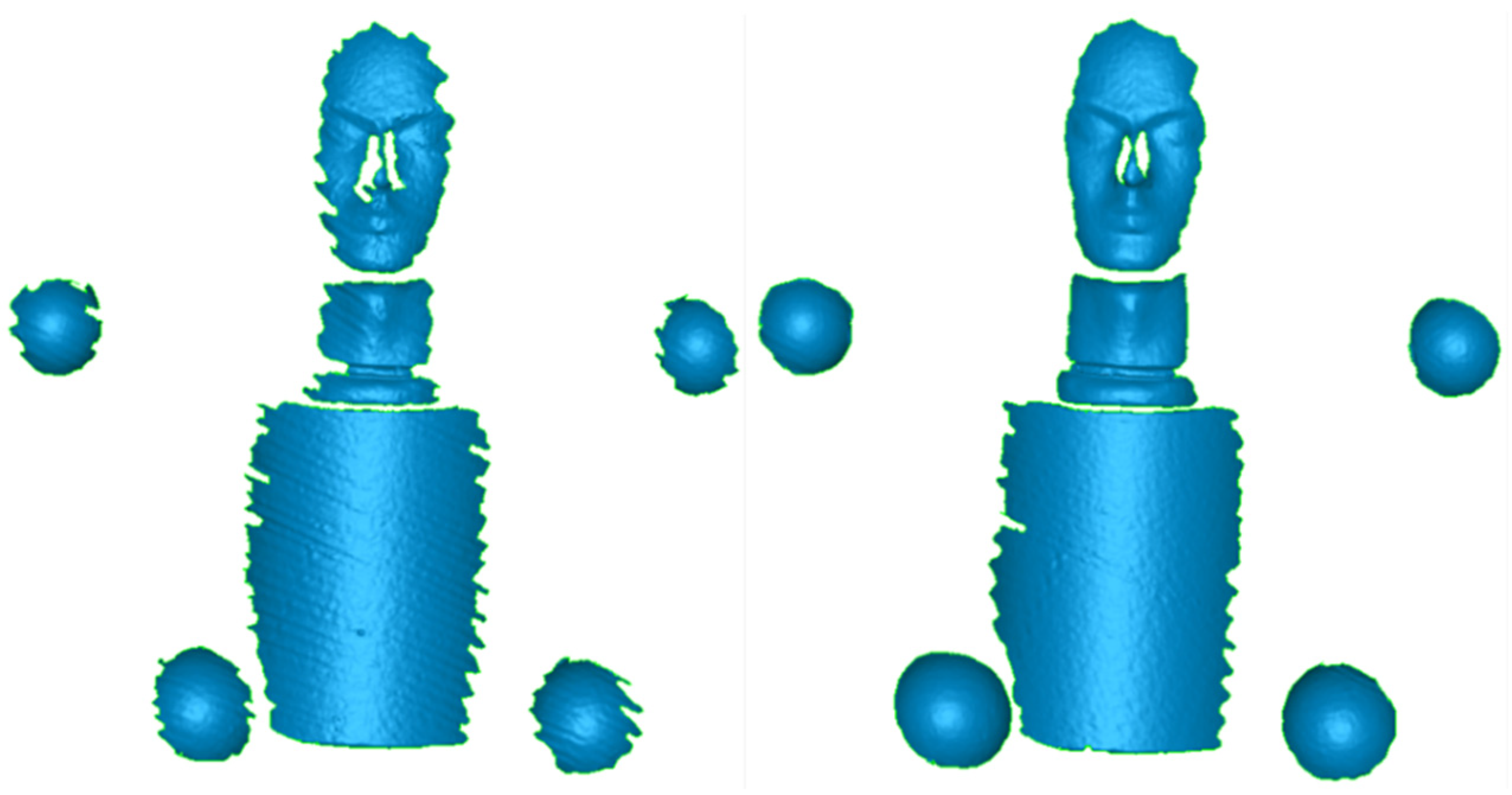
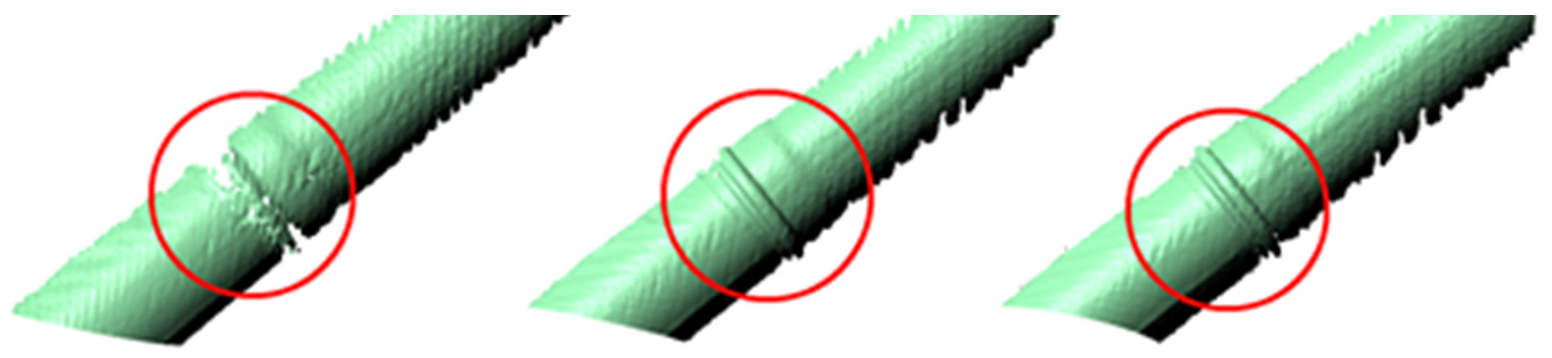
3.2. Measurements with Moved Sensor

First measurements with a moving sensor were performed in air in the laboratory. A constant linear motion with known velocity (0.2 m/s and 1.0 m/s) of the sensor was realized using a traversing track.

Video images were corrected using the known parameters for c, f, ps, and b and the estimated quantities d = d₀ = 2 m, v = 0.2 m/s (1.0 m/s), and α = 0°.

Figure 6 shows the resulting 3D point clouds of the measurement object cylinder, two ball bars, and a plaster bust without and with motion compensation at a velocity of 0.2 m/s and a 375 Hz 2D framerate. Results at 1.0 m/s velocity were not completely satisfying and should be improved in the future.

Subsequent experiments concerning motion compensation were performed in the water basin. Two different velocities were realized: 0.1 m/s and 0.7 m/s. The maximal sensor velocity of 1 m/s was not yet tested underwater. Motion compensation (MC) was realized manually (for reference), as well as automatically, using the implemented compensation algorithm. Figure 7 shows the results of manual and automatic motion compensation at 0.7 m/s velocity compared to the measurement result without motion compensation (left) with the example of a plastic pipe.

Table 3. Results of standard deviations of the 3D points from the fitted sphere and cylinder shape depending on sensor velocity and compensation method.

Velocity	Compensation Method	Standarddev. Sphere-Fit	Point Number on Sphere	Standarddev. Cylinder-Fit	Point Number on Cylinder
0.1 m/s	No	0.39 mm	6800	0.31 mm	69,000
0.1 m/s	Manually	0.31 mm	7100	0.32 mm	69,000
0.1 m/s	Automatically	0.33 mm	7100	0.32 mm	69,000
0.7 m/s	No	0.52 mm	3200	0.39 mm	47,500
0.7 m/s	Manually	0.36 mm	5200	0.34 mm	49,600
0.7 m/s	Automatically	0.32 mm	6000	0.34 mm	49,600

documents the standard deviations of the 3D points from the fitted sphere and cylinder shape, respectively. Motion compensation provides a significant reduction in the standard deviation. Automatic motion compensation gives comparable results to manual compensation.

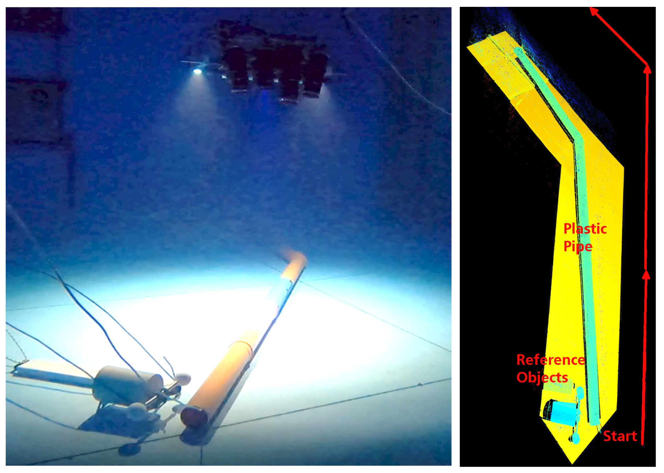
3.3. Measurement Example of 3D Model Generation by Registration of Consecutive Scans

Additional dynamic recordings were carried out using a triaxial gantry system. A pipeline was placed in the water, as well as the ball-bar specimen and plane normal. The underwater scene is shown in the left image of Figure 8. Tests were performed with two sensor velocities of about 0.1 m/s and 0.7 m/s. The sensor distance to the measurement objects was consistently approximately 2.0 m. The measurements were carried out in clear water with a temperature of about 14 °C. There was a negligible amount of stray light from the very small windows of the hangar.

The plastic pipe of about 7 m length on the floor of the basin was scanned in continuous motion of the sensor. Consecutive scans were merged according to the description in Section 2.3. The result is shown in the right image of Figure 8. The generated point cloud is composed of 680 individual scans. The point cloud is colored according to height.

4. Discussion

In this paper, we presented a new underwater 3D scanning device designed for offshore (up to 1000 m depth) inspection applications. The sensor captures the surface of objects continuously and builds up a 3D model of the scanned object in real time by moving along the object with velocities up to 0.7 m/s. The sensor was tested in a water basin under clear water measurement conditions.

The presented results of the new structured-light-based underwater 3D sensor mark a milestone in the development of such sensor systems concerning the achievable measurement accuracy. Results of static measurements of the specimens show that the systematic measurement error is in the same range of accuracy as 3D air scanners of comparable measurement volume. Additionally, using the 3D error compensation function, the systematic error decreased to below 0.2 mm, which is approximately 1/5000 of the measurement volume dimension. This is more accurate than some comparable air scanners. All these results were obtained in clear water under near-optimal extrinsic conditions. Hence, these results show the high accuracy potential of the device and not the real performance in possibly harsh conditions in real inspection applications offshore.

Compared to previously presented setups or devices based on the same 3D data generation principles [32,33,34], our new system provides a considerably larger measurement volume, longer object distance, and shorter exposure time (see

Table 4. Parameters of the 3D scanner compared previous devices based on structured illumination.

Device	Measurement Volume	Measurement Distance	Exposure Time
Ref [32]	0.5 m × 0.4 m × 0.4 m 1	1.0 ± 0.20 m	not specified
Ref [33]	0.5 m × 0.4 m × 0.2 m 1	1.0 ± 0.10 m	0.8 … 10 s
Ref [34]	0.25 m × 0.2 m × 0.1 m	0.4 ± 0.05 m	15 ms
UWS	0.9 m × 0.8 m × 0.8 m	2.0 ± 0.40 m	1 … 2.6 ms

¹ estimation according to the provided data in the cited paper.

). These features, together with the developed motion compensation method, make application with a fast continuously moving sensor possible.

The detected random errors are in the expected range. For precise measurements at high velocities, motion must be taken into account. The presented compensation via displacement in the image space already achieves a significant improvement in the application. This was shown by experiments with a traversing track in air and a gantry system for different speeds in water. Furthermore, the 3D output data, improved by motion compensation, allows for finer registration and thus the recording of more accurate 3D models. Experiments with a sensor velocity of 1 m/s must be conducted before offshore measurements can be performed.

The main task in future work is the extension of our experiments to offshore measurements under typical application conditions. These experiments should also analyze the influences of water turbidity, temperature, and salinity. Scattering effects of the particles in the water should also be studied. In order to simulate application at a 1000 m depth before real offshore experiments, we plan to test the UWS sensor system in an appropriate compression chamber.

Another task of future work is to realize an appropriate calibration method that can be effectively performed offshore, even under rough weather conditions.

References

1. Tetlow, S.; Allwood, R.L. The use of a laser stripe illuminator for enhanced underwater viewing. In Proceedings of the Ocean Optics XII 1994, Bergen, Norway, 26 October 1994; Volume 2258, pp. 547–555. [Google Scholar]
2. McLeod, D.; Jacobson, J.; Hardy, M.; Embry, C. Autonomous inspection using an underwater 3D LiDAR. In An Ocean in Common, Proceedings of the 2013 OCEANS, San Diego, CA, USA, 23–27 September 2013; IEEE: New York, NY, USA, 2014. [Google Scholar]
3. Canciani, M.; Gambogi, P.; Romano, F.G.; Cannata, G.; Drap, P. Low cost digital photogrammetry for underwater archaeological site survey and artifact insertion. The case study of the Dolia wreck in secche della Meloria-Livorno-Italia. Int. Arch. Photogramm. Remote Sens. Spat. Inf. Sci. 2003, 34, 95–100. [Google Scholar]
4. Roman, C.; Inglis, G.; Rutter, J. Application of structured light imaging for high resolution mapping of underwater archaeological sites. In Proceedings of the Oceans’10 IEEE Sydney, Sydney, NSW, Australia, 24–27 May 2010; pp. 1–9. [Google Scholar]
5. Drap, P. Underwater photogrammetry for archaeology. In Special Applications of Photogrammetry; Da Silva, D.C., Ed.; InTech: London, UK, 2012; pp. 111–136. ISBN 978-953-51-0548-0. [Google Scholar]
6. Eric, M.; Kovacic, R.; Berginc, G.; Pugelj, M.; Stopinsek, Z.; Solina, F. The impact of the latest 3D technologies on the documentation of underwater heritage sites. In Proceedings of the IEEE Digital Heritage International Congress 2013, Marseille, France, 28 October–1 November 2013; Volume 2, pp. 281–288. [Google Scholar]
7. Menna, F.; Agrafiotis, P.; Georopoulos, A. State of the art and applications in archaeological underwater 3D recording and mapping. J. Cult. Herit. 2018, 33, 231–248. [Google Scholar] [CrossRef]
8. Korduan, P.; Förster, T.; Obst, R. Unterwasser-Photogrammetrie zur 3D-Rekonstruktion des Schiffswracks “Darßer Kogge”. Photogramm. Fernerkund. Geoinf. 2003, 5, 373–381. [Google Scholar]
9. Bythell, J.C.; Pan, P.; Lee, J. Three-dimensional morphometric measurements of reef corals using underwater photogrammetry techniques. Coral Reefs 2001, 20, 193–199. [Google Scholar]
10. Harvey, E.; Cappo, M.; Shortis, M.; Robson, S.; Buchanan, J.; Speare, P. The accuracy and precision of underwater measurements of length and maximum body depth of southern bluefin tuna (Thunnus maccoyii) with a stereo–video camera system. Fish. Res. 2003, 63, 315–326. [Google Scholar] [CrossRef]
11. Dunbrack, R.L. In situ measurement of fish body length using perspective-based remote stereo-video. Fish. Res. 2006, 82, 327–331. [Google Scholar] [CrossRef]
12. Costa, C.; Loy, A.; Cataudella, S.; Davis, D.; Scardi, M. Extracting fish size using dual underwater cameras. Aquac. Eng. 2006, 35, 218–227. [Google Scholar] [CrossRef]
13. Galceran, E.; Campos, R.; Palomeras, N.; Carreras, M.; Ridao, P. Coverage path planning with realtime replanning for inspection of 3D underwater structures. In Proceedings of the IEEE International Conference on Robotics and Automation, Hong Kong, China, 31 May–7 June 2014; pp. 6585–6590. [Google Scholar]
14. Davis, A.; Lugsdin, A. Highspeed underwater inspection for port and harbour security using Coda Echoscope 3D sonar. In Proceedings of the Oceans 2005 MTS/IEEE, Washington, DC, USA, 17–23 September 2005. [Google Scholar] [CrossRef]
15. Guerneve, T.; Pettilot, Y. Underwater 3D Reconstruction Using BlueView Imaging Sonar; IEEE: New York, NY, USA, 2015. [Google Scholar] [CrossRef]
16. ARIS-Sonars. 2022. Available online: http://soundmetrics.com/Products/ARIS-Sonars (accessed on 17 March 2022).
17. Mariani, P.; Quincoces, I.; Haugholt, K.H.; Chardard, Y.; Visser, A.W.; Yates, C.; Piccinno, G.; Risholm, P.; Thielemann, J.T. Range gated imaging system for underwater monitoring in ocean environment. Sustainability 2019, 11, 162. [Google Scholar] [CrossRef] [Green Version]
18. 3DatDepth. 2022. Available online: http://www.3datdepth.com/ (accessed on 17 March 2022).
19. Moore, K.D. Intercalibration method for underwater three-dimensional mapping laser line scan systems. Appl. Opt. 2001, 40, 5991–6004. [Google Scholar] [CrossRef] [PubMed]
20. Tan, C.S.; Seet, G.; Sluzek, A.; He, D.M. A novel application of range-gated underwater laser imaging system (ULIS) in near-target turbid medium. Opt. Lasers Eng. 2005, 43, 995–1009. [Google Scholar] [CrossRef]
21. Duda, A.; Schwendner, J.; Gaudig, C. SRSL: Monocular self-referenced line structured light. In Proceedings of the 2015 IEEE/RSJ International Conference on Intelligent Robots and Systems (IROS), Hamburg, Germany, 28 September–2 October 2015; pp. 717–722. [Google Scholar]
22. Bleier, M.; van der Lucht, J.; Nüchter, A. Towards an underwater 3D laser scanning system for mobile mapping. In Proceedings of the IEEE ICRA Workshop on Underwater Robotic Perception (ICRAURP’19), Montreal, QC, Canada, 24 May 2019. [Google Scholar]
23. CathXOcean. 2022. Available online: https://cathxocean.com/ (accessed on 17 March 2022).
24. Voyis. 2022. Available online: https://voyis.com/ (accessed on 17 March 2022).
25. Kwon, Y.H.; Casebolt, J. Effects of light refraction on the accuracy of camera calibration and reconstruction in underwater motion analysis. Sports Biomech. 2006, 5, 315–340. [Google Scholar] [CrossRef]
26. Telem, G.; Filin, S. Photogrammetric modeling of underwater environments. ISPRS J. Photogramm. Remote Sens. 2010, 65, 433–444. [Google Scholar] [CrossRef]
27. Sedlazeck, A.; Koch, R. Perspective and non-perspective camera models in underwater imaging—Overview and error analysis. In Theoretical Foundations of Computer Vision; Springer: Berlin/Heidelberg, Germany, 2011; Volume 7474, pp. 212–242. [Google Scholar]
28. Li, R.; Tao, C.; Curran, T.; Smith, R. Digital underwater photogrammetric system for large scale underwater spatial information acquisition. Mar. Geod. 1996, 20, 163–173. [Google Scholar] [CrossRef]
29. Maas, H.G. On the accuracy potential in underwater/multimedia photogrammetry. Sensors 2015, 15, 1814–1852. [Google Scholar] [CrossRef]
30. Beall, C.; Lawrence, B.J.; Ila, V.; Dellaert, F. 3D reconstruction of underwater structures. In Proceedings of the 2010 IEEE/RSJ International Conference on Intelligent Robots and Systems, Taipei, Taiwan, 18–22 October 2010; pp. 4418–4423. [Google Scholar]
31. Skinner, K.A.; Johnson-Roberson, M. Towards real-time underwater 3D reconstruction with plenoptic cameras. In Proceedings of the IEEE/RSJ International Conference on Intelligent Robots and Systems (IROS), Daejon, Korea, 9–14 October 2016; pp. 2014–2021. [Google Scholar]
32. Bruno, F.; Bianco, G.; Muzzupappa, M.; Barone, S.; Razionale, A.V. Experimentation of structured light and stereo vision for underwater 3D reconstruction. ISPRS J. Photogramm. Remote Sens. 2011, 66, 508–518. [Google Scholar] [CrossRef]
33. Bianco, G.; Gallo, A.; Bruno, F.; Muzzupappa, M. A comparative analysis between active and passive techniques for underwater 3D reconstruction of close-range objects. Sensors 2013, 13, 11007–11031. [Google Scholar] [CrossRef] [PubMed]
34. Bräuer-Burchardt, C.; Heinze, M.; Schmidt, I.; Kühmstedt, P.; Notni, G. Underwater 3D surface measurement using fringe projection based scanning devices. Sensors 2016, 16, 13. [Google Scholar] [CrossRef]
35. Lam, T.F.; Blum, H.; Siegwart, R.; Gawel, A. SL sensor: An open-source, ROS-based, real-time structured light sensor for high accuracy construction robotic applications. arXiv 2022, arXiv:2201.09025v1. in print. [Google Scholar]
36. Furukawa, R.; Sagawa, R.; Kawasaki, H. Depth estimation using structured light flow-analysis of projected pattern flow on an object’s surface. In Proceedings of the IEEE International Conference on Computer Vision, Venice, Italy, 22–29 October 2017; pp. 4640–4648. [Google Scholar]
37. Catalucci, S.; Marsili, R.; Moretti, M.; Rossi, G. Point cloud processing techniques and image analysis comparisons for boat shapes measurements. Acta IMEKO 2018, 7, 39–44. [Google Scholar] [CrossRef]
38. Gaglianone, G.; Crognale, J.; Esposito, C. Investigating submerged morphologies by means of the low-budget “GeoDive” method (high resolution for detailed 3D reconstruction and related measurements). Acta IMEKO 2018, 7, 50–59. [Google Scholar] [CrossRef]
39. Leccese, F. Editorial to selected papers from the 1st IMEKO TC19 Workshop on Metrology for the Sea. Acta IMEKO 2018, 7, 1–2. [Google Scholar] [CrossRef]
40. Heist, S.; Dietrich, P.; Landmann, M.; Kühmstedt, P.; Notni, G. High-speed 3D shape measurement by GOBO projection of aperiodic sinusoidal fringes: A performance analysis. In Proceedings of the SPIE Dimensional Optical Metrology and Inspection for Practical Applications VII, Orlando, FL, USA, 17–19 April 2018; Volume 10667, p. 106670A. [Google Scholar] [CrossRef]
41. Luhmann, T.; Robson, S.; Kyle, S.; Harley, I. Close Range Photogrammetry; Wiley Whittles Publishing: Caithness, UK, 2006. [Google Scholar]
42. Bräuer-Burchardt, C.; Munkelt, C.; Gebhart, I.; Heinze, M.; Heist, S.; Kühmstedt, P.; Notni, G. A-priori calibration of a structured light projection based underwater 3D scanner. J. Mar. Sci. Eng. 2020, 8, 635. [Google Scholar] [CrossRef]
43. Bräuer-Burchardt, C.; Munkelt, C.; Gebhart, I.; Heinze, M.; Kühmstedt, P.; Notni, G. Underwater 3D Measurements with Advanced Camera Modelling. PFG-J. Photogramm. Remote Sens. Geoinf. Sci. 2022, 90, 55–67. [Google Scholar] [CrossRef]
44. Garrido-Jurado, S.; Muñoz-Salinas, R.; Madrid-Cuevas, F.J.; Marín-Jiménez, M.J. Automatic generation and detection of highly reliable fiducial markers under occlusion. Pattern Recognit. 2014, 47, 2280–2292. [Google Scholar] [CrossRef]
45. Kruck, E. BINGO: Ein Bündelprogramm zur Simultanausgleichung für Ingenieuranwendungen—Möglichkeiten und praktische Ergebnisse. In Proceedings of the ISPRS, Rio de Janeiro, Brazil, 17–29 June 1984. [Google Scholar]
46. Furgale, P.; Rehder, J.; Siegwart, R. Unified Temporal and Spatial Calibration for Multi-Sensor Systems. In Proceedings of the IEEE/RSJ International Conference on Intelligent Robots and Systems (IROS), Tokyo, Japan, 3–7 November 2013. [Google Scholar]
47. Shortis, M. Camera calibration techniques for accurate measurement underwater. In 3D Recording and Interpretation for Maritime Archaeology; McCarthy, J., Benjamin, J., Winton, T., van Duivenvoorde, W., Eds.; Springer: Cham, Switzerland, 2019; Volume 31. [Google Scholar]
48. Qin, T.; Li, P.; Shen, S. VINS-Mono: A robust and versatile monocular visual-inertial state estimator. IEEE Trans. Robot. 2018, 34, 1004–1020. [Google Scholar] [CrossRef] [Green Version]
49. Bleier, M.; Munkelt, C.; Heinze, M.; Bräuer-Burchardt, C.; Lauterbach, H.A.; Van der Lucht, J.; Nüchter, A. Visuelle Odometrie und SLAM für die Bewegungskompensation und mobile Kartierung mit einem optischen 3D-Unterwassersensor. In Proceedings of the Oldenburger 3D-Tage, 2022. in print. [Google Scholar]
50. Elseberg, J.; Borrmann, D.; Nüchter, A. Algorithmic solutions for computing accurate maximum likelihood 3D point clouds from mobile laser scanning plattforms. Remote Sens. 2013, 5, 5871–5906. [Google Scholar] [CrossRef] [Green Version]
51. VDI/VDE; VDI/VDE 2634. Optical 3D-Measuring Systems. In VDI/VDE Guidelines; Verein Deutscher Ingenieure: Düsseldorf, Germany, 2008; Parts 1–3. [Google Scholar]
52. Bräuer-Burchardt, C.; Kühmstedt, P.; Notni, G. Improvement of measurement accuracy of optical 3D scanners by discrete systematic error estimation. In Combinatorial Image Analysis, Proceedings of the IWCIA 2018, Porto, Portugal, 22–24 November 2018; Barneva, R.P., Brimkov, V., Tavares, J., Eds.; Springer: Cham, Switzerland, 2018; Volume 11255, pp. 202–215. [Google Scholar]
Figure 1. Laboratory setup of UWS.
Applsci 12 04139 g001
Figure 2. Sheets with ArUco markers combined with circle grids used for calibration.
Applsci 12 04139 g002
Figure 3. Specimen ball bars, plane-normal, and cylinder during evaluation measurements.
Applsci 12 04139 g003
Figure 4. Ball-bar length measurement results depending on object distance.
Applsci 12 04139 g004
Figure 5. False-color representation of flatness deviation: measurement distance of 1.7 m (above), 2.0 m (middle), and 2.4 m (below).
Applsci 12 04139 g005
Figure 6. 3D measurement results of the reconstruction of the air measurement with sensor velocity of 0.2 m/s without motion compensation (left) and with motion compensation (right). Note the higher completeness at the margins of the objects with motion compensation.
Applsci 12 04139 g006
Figure 7. 3D reconstruction result of underwater pipe measurement at 0.7 m/s sensor velocity without motion compensation (MC) (left), manual MC (middle), and automatic MC (right).
Applsci 12 04139 g007
Figure 8. Photograph of the sensor, pipe, and specimen (left) and false-color representation of the modeling result after merging of the continuously recorded 3D data sets (right).
Applsci 12 04139 g008