1. Introduction
From the beginning of aerial photography, which has been used for different tasks [
1,
2,
3,
4,
5], archaeologists realized the potential of this technique to study and discover new sites, because large areas of land could be analyzed more quickly, allowing them to understand the spatial organization of archaeological structures [
6]. Today, the range of image acquisition techniques in aerial archaeological research is vast; from satellites to small unmanned aerial vehicles (UAVs), these images can be produced in different visible light spectra (e.g., [
7]). This data source has opened new research perspectives for cultural heritage and archaeology at much vaster scales [
8,
9,
10]. The digital era has nevertheless produced a bottleneck. The use of large amounts of images is a problem since the images are often labeled manually or semi-automatically; this is a problem for humans due to the time required to label each archaeological structure [
11]. Fortunately, this repetitive task can now be tackled using methods based on machine learning [
12,
13]. The problem, in a nutshell, consists of the binary classification of pixels (structure versus other types of objects); we focus on object detection through supervised machine learning, particularly the detection of archaeological structures from satellite images with abundant vegetation [
14,
15,
16,
17]. Mesoamerican civilizations developed in Mexico, Guatemala, Belize, western Honduras, and El Salvador covering more than 300,000 km
2 [
18,
19]. There are still several unexplored and unstudied areas in this territory with hidden archaeological structures among the vegetation [
20].
Nowadays, digital image processing techniques, as well as computational learning algorithms, have been increasingly used by archaeologists for the discovery of new archaeological structures. Recently, F. Monna et al. [
21] proposed a method to detect from orthomosaics the enormous amount of dry stones used by past societies to build funerary complexes in the steppes of Mongolia. The problem with this method in sites with large amounts of vegetation, is obtaining reliable DEM maps, so, as F. Monna et al. commented, their method does not give good results in the jungle or wooded areas. In this work, we propose a method that allows the detection of archaeological structures in areas with a large amount of vegetation, from satellite images obtained with SASPlanet. For detection in these types of images, two color spaces (RGB and HLS) and different filters (Canny, Sobel, and Laplacian) were used; also, different supervised classifiers were tested. The experiments with different images taken from the archaeological sites of Calakmul, Comalcalco, Tikal, Zaculeu, Xcambó, Mayapán, Aké, and Palenque show that the proposed method achieves good results.
The work presented is organized as follows:
Section 2 contains the related work; in
Section 3 our proposed method is described; in
Section 4, some experiments carried out at different archaeological sites are shown; in
Section 5, we analyze our method and its limitations; and in
Section 6 our conclusions and future work are presented.
2. Related Work
According to UNESCO, armed conflicts and war, earthquakes and other natural disasters, pollution, poaching, uncontrolled urbanization, and unchecked tourist development pose significant problems to world heritage sites [
22,
23,
24,
25]. Due to this, records of archaeological structures have been generated worldwide through images. However, the amount of data makes analysis difficult. The development of artificial intelligence methods and approaches can help to facilitate the collection and understanding of the data in less time. Today, machine learning and computer vision techniques have assisted archaeologists in evaluating, predicting, and classifying their findings using images [
26,
27].
Literature shows different types of works that have used these techniques in the area of archaeology; for example, some works have been carried out to detect shipwrecks automatically through methods that use deep learning using elevation maps to apply new methodologies in the area of underwater archaeology, obtaining results that compete with or improve on those made by archaeologists [
28]. Another area in which these methods have been used is the classification of ancient artifacts, such as vessels from a Bronze Age cemetery in Saxony. The results exceeded archaeologists’ expectations by eliminating systematic errors within the typology [
15]. Artificial neural networks have also been applied to attributing the origins of archaeological ceramics by analyzing their composition found in different groups of archaeological sites, showing promising results [
17]. Another work focused on computer vision proposes a new representation of Mayan hieroglyphs that includes information from both the foreground and the background, obtaining better results than the state of the art [
29]; in a later work, a proposal was also made to improve this representation using thinned hieroglyphs by introducing an improved selection of points of interest which significantly improved the results of hieroglyph recovery [
30].
On the other hand, the work carried out by [
31] is based on monitoring and documenting archaeological sites in the Arctic using RGB images and thermal images obtained with the help of a drone. The results obtained by combining RGB and digital surface models helped to map the ruins and structures of the study sites. Similarly, Ref. [
32] focuses on identifying archaeological sites (tombs) in forested areas using time series of images with the help of machine learning. The results of this work indicate that the method works well for clustered tombs. Likewise, Ref. [
33] uses machine learning techniques with satellite images to detect Roman fortified sites in arid environments, obtaining results with an overall accuracy of 0.93 with field study data. Finally, Monna et al. [
21] use orthomosaics from the Jergalan area to analyze funerary complexes in Mongolia, using different machine learning algorithms to detect stone structures. The method uses different color spaces (RGB and HSV), textures (homogeneity, contrast, and entropy), and DEM maps and results in images that compete with or improve on the results obtained by archaeologists performing a manual classification. However, this method does not work well for jungle or wooded regions.
The use of image analysis and supervised classification is a tool that could serve to support archaeological research in different areas, such as the detection of archaeological structures, even in sites with large amounts of vegetation. All of the above motivates us to propose a new method that allows the detection of ancient structures in areas with large amounts of vegetation, such as those in the Mesoamerican region, which is introduced in the next section.
3. Proposed Methods
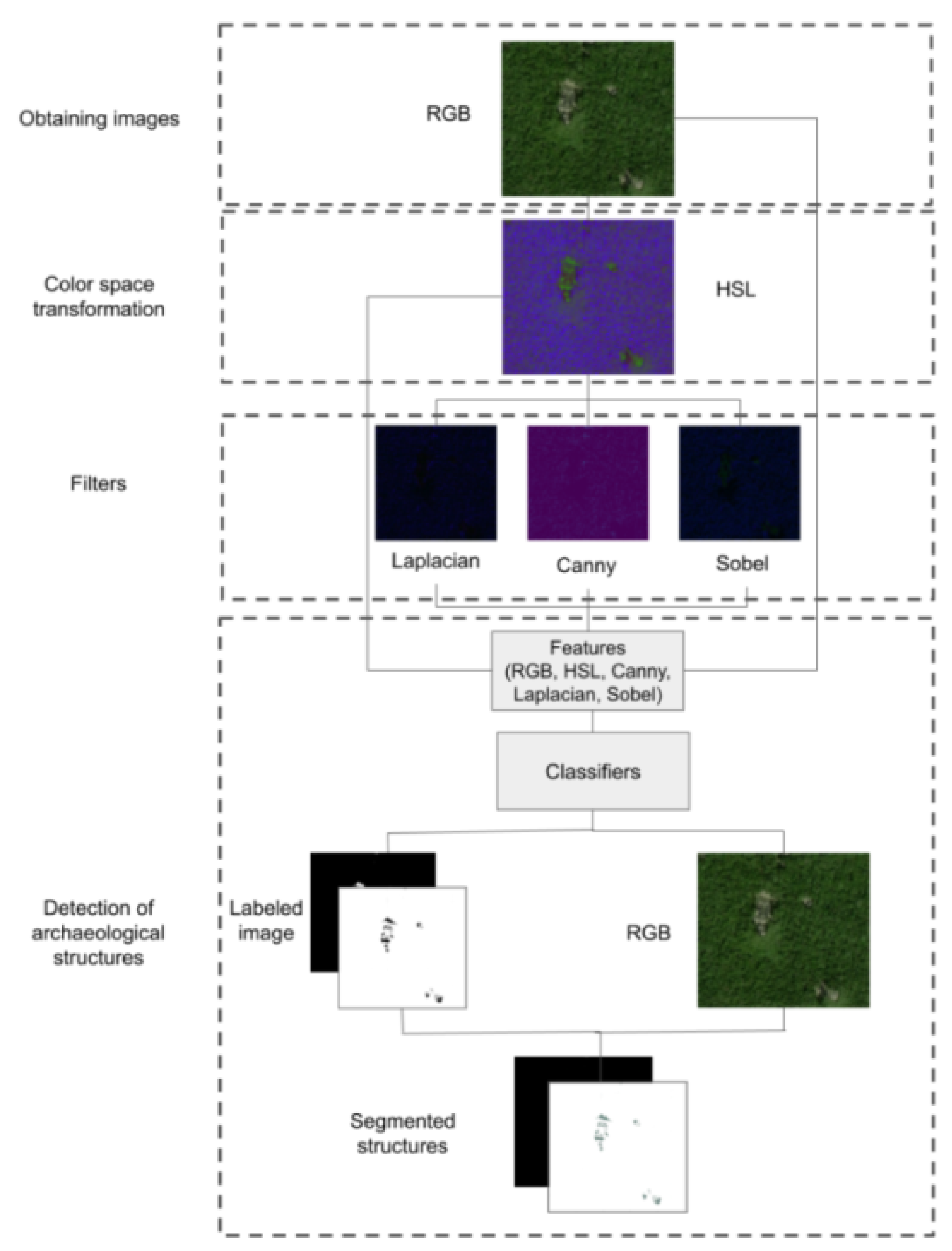
This work proposes a method to detect archaeological structures in jungle regions, such as Mesoamerican ones. First, we will broadly describe the proposed method, which uses satellite images from which useful features are extracted. With these features, we perform semantic segmentation of pixels of interest, in our case the archaeological structures, through a supervised classifier trained to detect these pixels. Later, the stages of our method will be explained in detail.
The proposed method receives an image of the site of interest in RGB color space. We propose applying a color space transformation (RGB to HSL) to generate a new image and use this new image to generate images with different filters. The color space transformation is necessary due to the type of filters we use. Once we have all the generated images (color spaces and filters), their channel values are used as features. Based on these features, a classifier is trained to perform pixel classification that detects the archaeological structure as part of the introduced method. As a result, we can build a new binary image where each white pixel corresponds to a pixel of an archaeological structure, and each black pixel corresponds to a pixel that does not belong to an archaeological structure. Finally, we use the RGB image and the binary image to remove all vegetation from the RGB image to isolate the archaeological structure, generating a segmented RGB image as a result. The general process followed by our proposed method can be seen in
Figure 1. In addition, we present a pseudocode Algorithm 1 that shows the process of our method. The following sections describe each stage of the proposed method in more detail.
| Algorithm 1 Workflow of our proposed method. |
- 1:
procedure Proposed method(rgbImage) Color space transformation - 2:
TransformRGBtoHSL(rgbImage) Filters - 3:
ApplyFilters(hslImage) Detection of archaeological structures - 4:
GenerateTrainingSet(rgbImage, hslImage, laplacian, canny, sobel) Classify Pixels - 5:
Classifier(trainingSet) Get Structure as image - 6:
GetStructurefromImage(rgbImage, pixelsclassified) - 7:
return structureImage - 8:
end procedure
|
3.1. Obtaining Images
The free application SASPlanet [
34] was used to obtain different images of the Mayan zone archaeological sites of Mexico and Central America. SASPlanet was designed for viewing and downloading high-resolution satellite images with the help of other servers such as Google Earth, Google Maps, Bing Maps, Nokia, Here, Yahoo, Yandex, OpenStreetMap, ESRI, and Navteq. The process followed to download the images was to identify the site of interest, select an area (see
Figure 2a), choose the image quality, select the image format (in our work, we use the .tif format, however, any other format can be used), select the post-processing options, and save the georeferenced information (see
Figure 2b). The image generated corresponds to the site of interest; the spectral range is from 380 to 700 (visible light), using three bands (RGB), with a spatial resolution of 15 m and a swath width at the nadir of 13.1 km.
Figure 2 shows the process followed to obtain the images using SASPlanet.
3.2. Color Space Transformation
Many color models are currently used because the science of color is a broad field encompassing many application areas [
7]. In this work, we use two color spaces (RGB and HLS), since transforming images to a non-RGB space has improved the classification performance [
35]. These two color spaces are described below:
RGB color space: The typical format involves a 24-bit encoding, where the image is constructed using three primary colors—red (R), green (G), and blue (B)—each represented by a separate channel that is processed by cameras and computers. With 8 bits allocated to each color channel, there are 256 distinct values possible per channel, resulting in a total of 16,777,216 color combinations. Additive color mixing is used in this color space to create the final image, which is divided into the three channels (R, G, and B) and treated as distinct features for each color channel.
HSL color space: This consists of three color channels: H (hue), which represents the primary colors (red, green, and blue); L (lightness), which takes into account the amount of light in an image, where the amount of light will tend to black; and S (saturation), where the amount of saturation in the image will depend on whether the color turns gray or maintains the original color. Choosing this color channel allows us to carry out the processing of the image in individual planes, because the color is represented in the image hue and lightness, while the saturation is used as a masking image that isolates the area of interest in the image [
7].
The change in the color space from RGB to HSL in our experiments helped us to obtain images with filters that contain more information due to the composition of the HSL. The tests can be seen in
Figure 3, where we can see images generated from these color spaces with the help of different filters. This figure shows that the filters (especially the Canny and Laplacian filters) emphasize more pixels corresponding to vegetation in the HSL color space than in the RGB color space.
3.3. Filters
Filters are used to achieve specific objectives when processing digital images. These objectives include reducing the number of intensity variations between adjacent pixels, which is known as smoothing the image. Another goal is to eliminate noise, which involves identifying and removing pixels with intensity levels that differ significantly from their neighbors. Such noise can originate from the image acquisition or transmission processes. Filters can also be used to boost edges, highlighting the edges located in an image, or to detect edges, which refer to pixels with sharp changes in intensity. These operations are applied to the pixels of an image to optimize it, emphasize specific information, or achieve a particular effect. The filtering process can be performed in the frequency domain and/or color space [
36].
For better feature extraction (structure versus non-structure), we tested mean, median, variance, convolution, bilateran, Canny, Laplacian, and Sobel filters. However, we selected the Canny, Laplacian, and Sobel filters, because they produced better results than the others, allowing us to improve the detection of archaeological sites in areas with a lot of vegetation.
The Canny filter is based on the first derivative of a Gaussian function. However, since raw image data is often affected by noise, the original image is preprocessed with a Gaussian filter to reduce the noise. This results in a slightly blurred version of the original image [
37].
The Laplacian filter on the other hand, is an edge detector that calculates the second derivatives of an image, measuring the rate of change in the first derivative. It is used to determine whether a change in adjacent pixel values represents an edge or a continuous progression [
37].
Finally, the Sobel filter uses a small, separable, integer-valued filter in both the horizontal and vertical directions to convolve the image. This filter is relatively inexpensive in terms of runtime [
37].
The objective of using the different images generated from the RGB image is to include different features (information) in images, to improve the detection of archaeological structures by a classification algorithm.
3.4. Detection of Archaeological Structures
This stage aims to determine whether or not a pixel in the image corresponds to an archaeological structure. This is achieved by applying a supervised classifier that uses a training set of previously labeled pixels, using images generated with the color spaces (RGB and HSL) and filters (Canny, Laplacian, and Sobel). In this way, the pixels of new images can be classified using the information of the pixels in the training set. In our proposal, the labeling of the pixels in the training set was carried out manually using the ImageJ software (
https://imagej.nih.gov/ij/, accessed on 14 May 2023). For this, we created a few rectangles on areas defined as “structure” or “non-structure”, and all pixels in each rectangle were labeled accordingly. Each pixel of type “structure” and “non-structure” is described through a feature vector with 15 entries, each one corresponding to the pixel values in each channel of the RGB and HSL images, and the pixel values in each channel after applying the three filters (Canny, Laplacian, and Sobel) on the HSL image. Thus, we obtain vectors as follows:
. The labeling described produces a set of pixels of structure type or non-structure type described by fifteen features, constituting the training set for a supervised classifier.
Figure 4 shows an example of the pixels selected as a training set for the Calakmul area. This image corresponds to the RGB color space, showing the structure (red) and non-structure (blue) type pixels. This example shows that the number of pixels selected as a training set is very small and easy to obtain compared to manually labeling the whole image. Additionally, using a small training set positively impacts the time required for training a classifier. Once the training set is built, a classifier will train a model to classify all of the image pixels as structure or non-structure, i.e., detect (if it exists) the archaeological structure based on the small training set.
4. Experiments
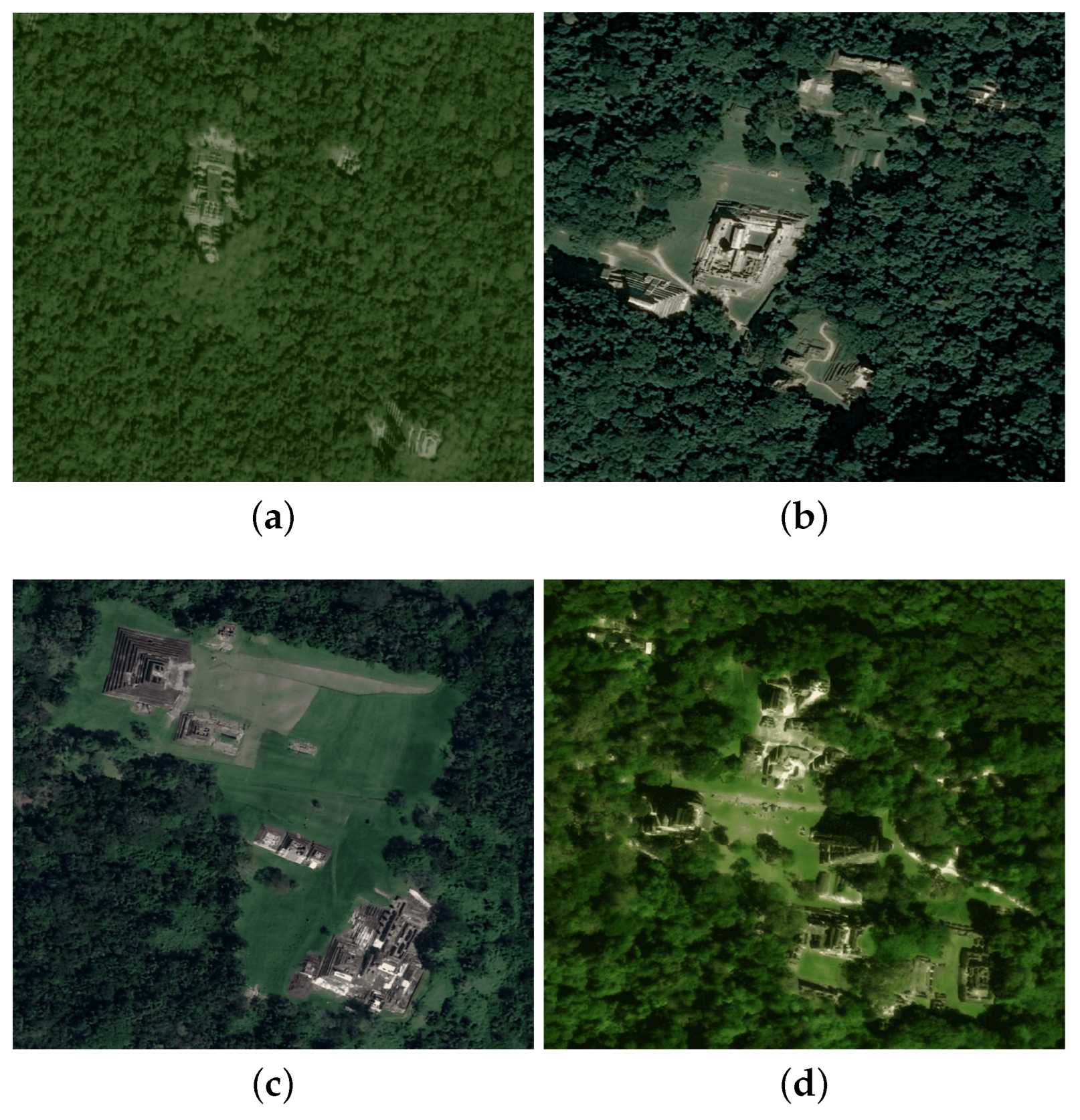
To assess the proposed method, we applied it to images of four archaeological sites: Calakmul, Palenque, Comalcalco, and Tikal. For this, we manually selected small training sets of pixels, as explained in the previous section. Some images of the archaeological sites used in this experiment can be seen in
Figure 5. To show the performance of our proposal, we performed three evaluations. First, we evaluated our method by applying five-fold cross-validation on the selected training set. As a second evaluation, we used the chosen training set on an image to classify all of the pixels in the image. Then, we assessed the classification by comparing the classifier’s result against the fully labeled image. Finally, a third evaluation is presented to show the performance of our proposal in a more realistic scenario; for this, we used high-resolution satellite images and graphically show the archaeological structures detected by our proposed method.
For our first evaluation, we selected training sets from four archaeological sites: Calakmul, Palenque, Comalcalco, and Tikal. For this, a training set was created for each archaeological site, manually selecting rectangles of different sizes on areas with structures and non-structures.
Table 1 shows the sizes of the training sets for each archaeological site. Since the selection was made manually, the number of pixels selected for each image varies due to the size of the selected rectangles. The pixels selected for the Calakmul area can be seen in
Figure 4.
To evaluate the performance of our proposal, we used the training set and applied five-fold cross-validation over this set to obtain an evaluation of the classifiers. This process consists of creating five subsets called folds, each with 20% of the training set, each containing the same proportion of structure and non-structure pixels as the whole training set. Then, we took four folds to train the classifier and one fold to test the classifier and evaluate its classification quality. This process was repeated five times, taking each of the five folds as a test set. Finally, the value reached by the quality measures in each of the five evaluations was averaged and reported. Although semantic segmentation is a major part of our work, we decided not to use segmentation-based performance measures such as IoU and BF score since, in a real scenario, the images are not apriori whole segmented. Thus, the measures used to evaluate the classifier in our experiment were: precision, recall, F1 score, and accuracy, since they are widely used to evaluate the performance of a classifier. To compute these metrics, it was necessary to know the values TP (true positive = number pixels of structure correctly classified as structure), TN (true negative = number pixels of non-structure correctly classified as non-structure), FP (false positive = number pixels of non-structure wrongly classified as structure), and FN (false negative = number pixels of structure wrongly classified as non-structure), where the positive class corresponds to structure pixels, and the negative class corresponds to non-structure pixels. To obtain these measures the following equations were used:
Table 2 shows the results obtained with different metrics using different supervised classifiers: KNN (K-nearest neighbors, using Euclidean distance with a value of K = 5), NN (neural networks, with an Adam optimizer, a hidden layer size of (5, 5, 7), a learning rate of 0.001, an alpha value of 1 ×
, and an epsilon of 1 ×
), RF (random forest, with a number of trees of 20 and a maximum depth of 3), SVM (support vector machines, using a polynomial kernel), and LR (logistic regression, with a liblinear optimizer and a maximum of 1000 iterations). In
Table 2, we can see that most of the values are higher than 0.98, because the results were obtained based just on the pixels of the training set.
The second evaluation uses a fully labeled image to assess the classification of unlabeled pixels in our proposed method. Thus, we select a small training set, as explained in the previous section. The pixels in the whole image are labeled by applying our method, and, using the same metrics, the classifier’s quality is evaluated. These metrics were obtained by comparing the pixels labeled by the classifier against the correct label in the fully manually labeled image. The image used for this experiment corresponds to a small portion of the high-resolution image of the archaeological site of Calakmul. It contains an image with a size of 599 × 512 pixels. The pixels selected for the training set in this image were 142 for structure and 256 for non-structure.
Figure 6 shows this small image and the pixels selected for the training set.
Figure 7 shows the fully labeled image, where the yellow outline delimits the areas corresponding to the archaeological structure. We manually labeled this image. The results obtained can be seen in
Table 3, where we can see that these results are lower than those obtained in the previous experiment. This happens because the classifier wrongly labeled some pixels as non-structure compared to the fully labeled image. The labeling error is due to the shadows contained in the structures. However, these results are fairly good, from 92% to 97%.
We show how our proposed method works in practice as a third evaluation. For this, we use large images from each of the archaeological sites. As an example, we only show the results obtained using our method on the image of the Calakmul site. For the other sites, we only show the image of the detected archaeological site output by our method. We selected Calakmul to show all the steps of our method because large amounts of vegetation hide it. However, the images of all the steps corresponding to the other archaeological sites and their results can be seen and downloaded from (
https://ccc.inaoep.mx/~ariel/Detection-of-archaeological-structures/, accessed on 14 May 2023). For the Calakmul site, the image in the HSL color space, as well as the filters (Laplacian, Canny, and Sobel), were generated and can be seen in
Figure 8. In this figure, we can notice, especially in the HSL image, that a large part of the vegetation can be differentiated, which is a good result of our method. However, this does not always happen with all images. On the other hand, it can be seen that the Canny and Laplacian filters can better represent the vegetation, and the Sobel filter can emphasize the edges of the structure.
Since all of the classifiers obtained similar results, we only show the results obtained with the neural network (NN) classifier.
Figure 9b shows the binary image generated by this classifier. This figure shows that a large part of the vegetation was correctly labeled if we compare it with
Figure 9a, so our method detected the structure pixels successfully. However, it is important to mention that the shadows in the images affected the classification of the pixels, since the structure pixels in shadow are similar to vegetation pixels in shadow. Therefore, providing images free of shadows to the classifier is advisable since it can help the classifier generate better classification results, producing better archaeological site detection.
Using the binary image generated by the classifier, we segmented the archaeological site detected by our method in the RGB image by changing the color of the pixels labeled as non-structure to black. Thus, we isolate the archaeological structure from the vegetation. The obtained results can be seen in
Figure 10b, where we can appreciate a large part of the structure was correctly segmented if we compare it with
Figure 10a.
Figure 11 shows the results obtained in the Palenque, Comalcalco, and Tikal archaeological sites, showing the images in RGB and the segmented RGB images. The archaeological sites of Palenque and Comalcalco obtained the best results since the quality of these images is better. The errors in Tikal’s and Calakmul’s images are due to the shadows and the soil’s similarity with the archaeological structure. So it was not easy for the classifier to discriminate between structure and non-structure pixels.
Finally, to validate our proposed method, we trained our classifiers using another archaeological site (Dzibilchaltun) and analyzed the results on archaeological sites such as Xcambó, Mayapán, and Aké. We used only one satellite (Google Maps) to obtain these images, because using different satellites would produce different-resolution images, affecting the classifiers’ performance. The obtained results can be seen in
Figure 12. As shown in
Figure 12, our proposed method can detect archaeological sites without prior labeling, with good results.
5. Discussion
Although at first sight, it seems that just by looking with the naked eye at the RGB image it is possible to distinguish pixels belonging to an archaeological structure from pixels not in the structure, for computers performing this task is not so immediate. From the experiments, we can see the usefulness of our proposed method to more quickly identify archaeological structures in large areas of land with a lot of vegetation. Our method reduces archaeologists’ pixel selection time when identifying large-image structures. Eventually, our method allows the archaeologist not to waste time on this task, allowing them to perform more significant duties. Our experiments also showed that using appropriate filters and color spaces, and their synergy with a supervised classifier, made possible the detection of archaeological structures. The difference between our method and other approaches is that our method focuses on images with large areas of land and a lot of vegetation. Hence, using color spaces and filters was vital to highlighting information helpful to the classifier.
The main limitation of our method is in images with shadows (due to vegetation, structures, and weather), which caused the classifiers to be unable to discriminate between archaeological structures and vegetation. Additionally, we noticed that some structures partially covered by grass, trees, or soil also caused classification errors. This type of image remains a challenge that deserves study in future work. However, as we showed in our experiments, the results obtained with our proposal are suitable for detecting archaeological structures in areas with a lot of vegetation which are usually difficult to access.

 ,
, 


