Operation Optimization of Medium-Depth Ground Source Heat Pump (MD-GSHP) Systems Based on the Improved Particle Swarm Algorithm

Abstract

In recent years, the medium-depth ground source heat pump (MD-GSHP) has become a promising and potential geothermal energy heating technology. This is due to the superior characteristics of buried pipes with a small diameter, the high energy efficiency of the heat pump, the insensitivity to the ground climate, and other conditions. Among currently available studies, both the variable operating conditions and the addition of thermal storage devices have rarely been considered. Despite this, the optimization methods applied to the medium-depth GSHP system are relatively simple. In this paper, an MD-GSHP system, including the thermal storage device with variable operating conditions, was fabricated. The operation strategies of the system were optimized by employing the improved particle swarm algorithm after applying the operating costs, the coefficient of performance of the system (COP) and the geothermal energy utilization coefficient to the objective functions, and the optimization results were compared and analyzed. The results show that the predictions of the optimized operating costs, the COP of the system, and the geothermal energy utilization coefficient were found to be CNY 279.27, 6.4420, and 0.8527, respectively. The effect of the COP on the optimization effect was opposite to that of operating costs, but analogous to that of the geothermal energy utilization coefficient.

1. Introduction

As a clean and renewable energy source, geothermal energy is characterized by a stable energy supply, large storage capacity, and wide distribution. As such, the use of geothermal systems for building heating has been increasing worldwide in recent decades. As it has no carbon footprint, ground source heat pump (GSHP) heating technology has a significant potential for continued development. The application of this technology will help mitigate smoke and haze occurring during winter in northern China, which results from coal combustion heating. Generally, according to the ground depth of heat extraction, GSHP roughly includes two categories of the shallow-depth GSHP and the medium-depth GSHP (MD-GSHP). As shallow-depth GSHP heating technology occupies a large area and has difficulty maintaining the thermal balance of the soil, the promotion and application of this technology has been limited. In 2012, medium-depth GSHP heating technology was proposed by some scientists in China, and it has been rapidly promoted in Shaanxi, Henan, and Beijing in northern China. For medium-depth GSHP heating technology, a closed-cycle water system is adopted to extract heat from the high-temperature rock and soil layer 2~3 km underground; this is achieved by drilling holes and installing medium-depth buried pipe heat exchangers in them. Then, heat from water as a heat transfer fluid (HTF) drives a high-temperature heat pump to heat the buildings [1]. Compared with shallow-depth GSHP technology, the underground heat-exchanging area of the buried pipe exchanger for MD-GSHP is smaller; this benefit comes in addition to the higher heat pump efficiency. Furthermore, MD-GSHP is not sensitive to ground temperature and other surrounding conditions [2].

At present, increasing amounts of attention have been paid to medium-depth GSHP systems in China. Numerical simulations on the heating coefficient of performance and optimization of the system have been conducted. The optimization of the MD-GSHP system was primarily carried out on the two kinds of variables of operating parameters, including the circulation flow and operation stop ratio, and the design parameters, including the space between boreholes, the nominal diameter of the buried pipe, the run-stop ratio, etc. Taking an 8000 m² residential building in Harbin, China, as a case study, Zhang [3] emulated the operational energy efficiency of the GSHP units and the water system of the ground source side in the GSHP system at constant and variable flowrates under certain operating variables. Ren et al. [4] analyzed the variations in the unit, buried pipe, and heating terminal under three operation conditions of intermittent mode GSHP through an experimental study on the operation modes of the MD-GSHP system in some severely cold regions. Deng et al. [5] tested the operational performance and energy efficiency of the medium-depth GSHP system in Xi’an. In their study, the energy efficiency of the medium-depth GSHP system and the heat transfer performance of the geothermal heat exchanger were revealed by the results of short-term and annual field tests. Pratiwi et al. [6] quantified the life cycle impacts of six heating and cooling configurations from shallow to medium-depth geothermal wells with connected, decentralized heat pumps and district heating and cooling in the State of Geneva. Zuo et al. [7] adopted the residential community heating in Fuxin City, Liaoning Province as an example and established a simulation model by TRNSYS software. In addition, they investigated the effect of variables that could determine the annual costs of the medium-depth double U-shaped buried pipe heat pump system through simulation and orthogonal tests. Wang [8] took the medium-depth GSHP system in Handan City, Hebei Province as an engineering case, along with proposing a simulation model of the medium-depth GSHP system. According to this model, they investigated the influence of different combinations of circulating flow rates on the operating efficiency of the system under different load demands, as well as the optimal operation strategy for the long-term operation of the medium-depth GSHP system. Du et al. [9] took the office building in Xi’an, Shaanxi Province as an example and studied the design load ratios of the medium-depth GSHP system with auxiliary heat sources in Northwest China, while the energy consumption, economic evaluation, and the emission of environmental pollutants were analyzed for a medium-depth geothermal energy-coupled gas boiler heating system at different design load ratios. Ma et al. [10] adopted the technology of a direct heat exchange of geothermal water coupling cascade utilization and the exchange of production wells and reinjection wells, developing the central heating of a residential district of Xianyang. Wang et al. [11] conducted field experiments on the performance of the deep borehole heat exchanger at multiple depths (400 m–2000 m) in a ground source heat pump system in Harbin. The results indicated that the heat extraction capacity climbs linearly with the increase in the borehole depth. Guo et al. [12] made a measurement for a medium-depth geothermal heat pump system with a depth of 3183 m in Shanxi Province, including the average initial soil temperature, heat exchange capacity, and operation parameters.

Particle swarm optimization (PSO) is a swarm intelligence algorithm which can be used to deal with various optimization and scheduling problems, and it has been applied in many fields. Zhao et al. [13] proposed an improved particle swarm optimization algorithm (IPSO) to the optimal reactive power dispatch and voltage control of power systems. Simulation results demonstrate that the proposed approach is superior to current methods for finding the best solution, in terms of both the solution’s quality and algorithm’s robustness. Mussetta et al. [14] proposed some variations over the basic particle swarm algorithm and applied them to a mathematical test function and to a microwave microstrip filter. The results show their superior capabilities with respect to the conventional version. Zhang et al. [15] used an improved particle swarm optimization algorithm to solve a DNA encoding problem and integrated it into required combinatorial and thermodynamic constraints for DNA computing. Gu et al. [16] used the principle depressed SSR by STATCOM and chose appropriate measured data to design sub synchronous damping control (SSDC) based on an improved particle swarm optimization algorithm. The subsystem within the Mohong and Yanchong series capacitors of the China Southern Power Grid was taken as an example to verify the validity of SSDC. Liu et al. [17] adopted an improved particle swarm optimization algorithm in the CDMA multiuser detection (MUD). The result shows that the algorithm accelerates the convergent speed, yet it also displays feasibility and superiority in case simulation. Ma [18] suggested an improved particle swarm optimization algorithm to deal with the hydropower station optimal operation. Compared with the particle swarm optimization algorithm, the simulation results of the new algorithm show an improved convergence speed and computational accuracy. Kumar et al. [19] developed three improved PSO algorithms, IPSO-A, IPSO-B, and IPSO-C, to solve an economic load dispatch (ELD) problem for IEEE 5, 14, and 30 bus systems. The results show that the proposed improved PSO techniques provides the optimum operating cost with consistent results in terms of the diversity of the results. Cao et al. [20] proposed an improved particle swarm optimization algorithm and improved the key parameters to enhance the performance of the algorithm. The results show that, under parallel mode, the operation cost of the micro-grid decreases by 2.9% by applying IPSO the algorithm compared to the other algorithm of PSO, while the operation cost is only 2.7% from the original algorithm under islanding mode. Song et al. [21] proposed an optimization of pulse CVT based on an improved particle swarm algorithm. The results show that the accuracy and robustness of the improved particle swarm algorithm is improved by an order of magnitude, the solution time is reduced by 70%, and the optimal transmission speed is decreased by about 41%. Luo et al. [22] used the algorithm based on improved particle swarm optimization to detect the optimum drainage route in the current environment and proposed an intelligent scheduling method for the drainage routing problem in drainage pipe network. Luo [23] proposed a grid harmonic estimation method based on the particle swarm optimization algorithm. The improved particle swarm optimization algorithm was used to simulate the dynamic voltage signal, and the parameter estimation effects in different noise environments were compared. Wang et al. [24] introduced the idea of neighborhood particles into the standard particle swarm optimization algorithm and proposed a furnace flame recognition method based on the improved particle swarm optimization algorithm. Ahmadi et al. [25] improved the particle swarm algorithm to solve the problem of optimal keying angles for inverters. The simulation results represent the high efficiency of the improved type of particle swarm algorithm in determining the appropriate angle of fire for reducing the high harmonics and generating a waveform with a very low harmonic distortion and near sinusoidal. Tao et al. [26] proposed an improved particle swarm optimization algorithm to solve the AGV path planning problem of a one-line production line in the workshop. The experimental results show that the algorithm can improve the efficiency of AGV in material transportation and verify the effectiveness of the related improvement mechanisms. Cai [27] proposed a dormitory allocation method oriented around the heuristic particle swarm genetic algorithm, which uses a traditional greedy algorithm, heuristic improved particle swarm algorithm, and improved genetic algorithm to optimize the randomly allocated dormitory sequence. Feng et al. [28] improved and applied the adaptive particle swarm optimization algorithm to the study of statistical model fitting of atmospheric turbulence profiles. The simulation results show that the proposed method has a similar convergence accuracy to other adaptive particle swarm optimization algorithms, but the speed is faster.

In 2018, Ioakimidis, C. S. et al. [29] established a mathematical model to peak-shave and valley-fill the electricity consumption of non-residential buildings by managing the charging/discharging process in an electric vehicle parking lot to stabilize the load. Fang C. et al. [30] discovered that the COP (coefficient of performance) of the heat pump was affected by the partial load rate and outdoor temperature. They proposed a method to reduce the operation cost of the heat pump by adjusting the temperature and mass flow rate of supply and return water, and the results showed that the operation cost could be saved by 20–30%. Bandyopadhyay A. et al. [31] analyzed a community’s appliances, such as their HAVC (heating, ventilation, and airconditioning) systems, electric boilers, electric cars, and water pumps. They found that the time-varying power price could encourage residents to concentrate power consumption from peak hours to valley hours on the premise of not incurring a significant inconvenience. Nouri G. et al. [32] performed a calculation of three configurations of a combined solar evacuation collector and ground source heat pump. They found that the indirect expansion of the collector in parallel had the highest COP (3.96), which was superior to those of a direct expansion and indirect expansion in series.

Among the currently available studies, not only the variable operating conditions and the addition of thermal storage devices are rarely considered; furthermore, the optimization methods applied for the medium-depth GSHP system were relatively simple in these studies. In this study, a medium-depth GSHP system including the heat storage device was fabricated, in which the variable working conditions of GSHP were adopted, while the improved particle swarm algorithm was applied to optimize the system operation under different objective functions. In addition, the heating load distribution by hot water storage and by the heat pump in peak time, as well as the heating load and thermal energy storage load by the heat pump in valley time, were optimized. Additionally, the optimization results were compared and analyzed.

Compared to the traditional system (a heating system without thermal energy storage) and system with thermal storage in the literature, the proposed system meets a variety of operating conditions over the course of one day, which is beneficial to develop the stability of power consumption. In addition, because a lot of the load is transferred from peak hours to valley hours and flat hours, the electric fee decreases, and the fluctuation in power is suppressed during the whole heating season as well.

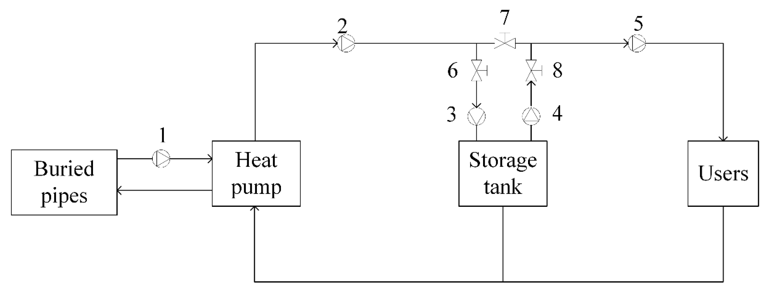
2. System Description

As shown in Figure 1, in order to meet the demand of a maximum heating load of 230 kW for a residential building with an area of 4000 m² in Xi’an, China, a MD-GSHP system was fabricated, including the medium-depth buried pipes, heat pump units, heat storage tanks, water pumps, and pipelines.

The working principle of the system is as follows: the working fluid in medium-depth buried pipes extracts heat from the underground rock and soil around the drilled hole. When the fluid flows through the GSHP, its temperature is increased. After fluid with a higher temperature heats the building, it flows back underground to repeat the next heat extracting circulation. As for the setting of the water storage tank, this is for the consideration of balancing the heat supply and demand in real time. When the heat supply from geothermal energy and GSHP is greater than the heat demand of the building, some of fluid will be stored in the heat storage tank. On the contrary, the water in the heat storage tank will be pumped out for a heating cycle.

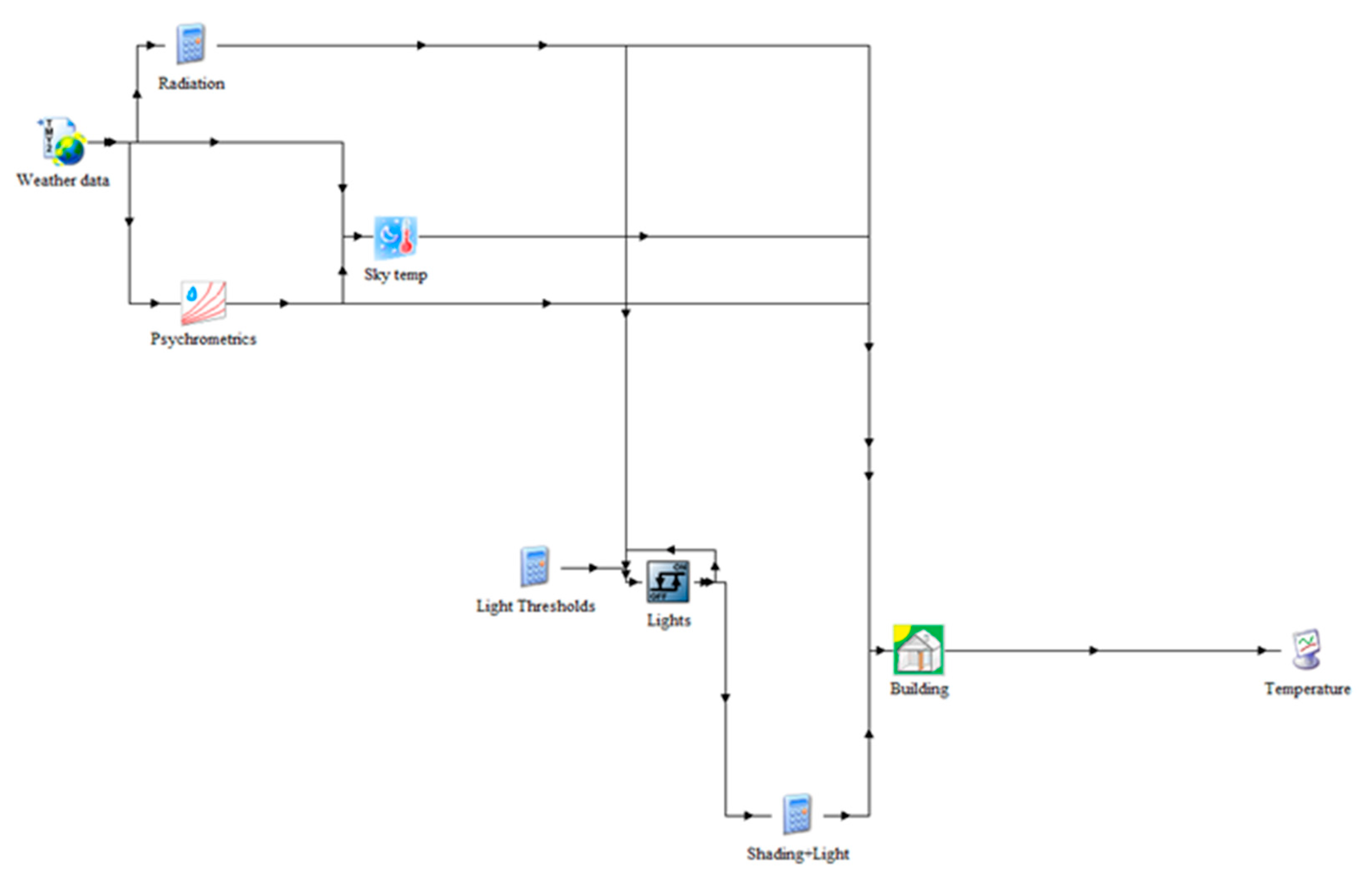
2.1. Calculation of Heating Load

Before the formal simulation, the user’s heating load should be obtained first. As Figure 2 shows, the building model was built in TRNSYS. The indoor temperature was kept at 20 °C and the heating load of the building was calculated.

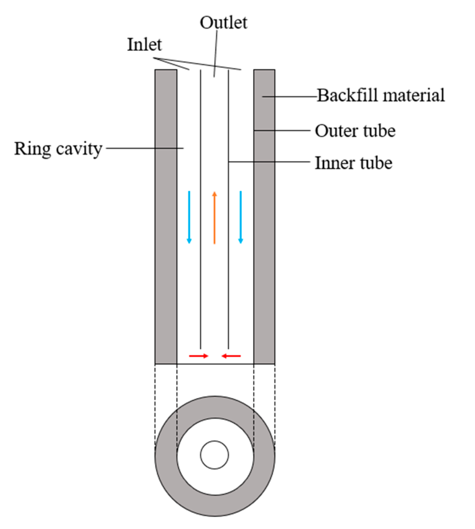
2.2. Buried Pipe Model

As shown in Figure 3, the buried pipe is a coaxial casing structure in which water, as the working medium, flows into the annulus, absorbs heat from the surrounding rocks and soil, and then flows out of the inner pipe. Besides the constant temperature difference between the water and formation, some basic parameters applied to the operation mode are listed in

Table 1. Basic parameters of buried pipe.

Parameter	Value
Drilling depth	2000 m
Drilling diameter	0.28 m
Outer diameter of outer tube	177.8 mm
Inner diameter of outer tube	159.42 mm
Outer diameter of inner tube	110 mm
Inner diameter of inner tube	90 mm
Thermal conductivity of outer tube	41 W/(m·K)
Thermal conductivity of inner tube	0.4 W/(m·K)
Thermal conductivity of backfill material	1.8 W/(m·K)

.

The governing equations applied in the buried pipes are expressed as follows: Energy equation of the ring cavity:

$$\rho q_{v}c\frac{\partial T_{\mathrm{f}1}}{\partial z}=\frac{T_{\mathrm{s}}-T_{\mathrm{f}1}}{R_1}+\frac{T_{\mathrm{f}2}-T_{\mathrm{f}1}}{R_2}$$

(1)

Energy equation of the internal cavity:

$$\rho q_{v}c\frac{\partial T_{\mathrm{f}2}}{\partial z}=\frac{T_{\mathrm{f}1}-T_{\mathrm{f}2}}{R_2}$$

(2)

where $\rho$ is the density of the circulating mass, kg·m⁻³. $q_v$ is the flow rate of the circulating mass, m³·s⁻¹. $c$ is the specific heat capacity of the circulating mass, J·kg⁻¹·K⁻¹. $R_1$ is the thermal resistance of the underground rock to the ring cavity fluid, m·K·W⁻¹. $R_2$ is the thermal resistance of the ring cavity fluid to the inner cavity fluid, m·K·W⁻¹.

The thermal resistances $R_1$, $R_2$ are calculated by Equations (3) and (4):

$$R_1=\frac{1}{h_1\mathsf{\pi }{d}_{1\mathrm{i}}}+\frac{1}{2\mathsf{\pi }{\lambda }_{\mathrm{p}1}}\ln \left(\frac{d_{1\mathrm{o}}}{d_{1i}}\right)+\frac{1}{2\mathsf{\pi }{\lambda }_{\mathrm{b}}}\ln \left(\frac{d_{\mathrm{b}}}{d_{1\mathrm{o}}}\right)$$

(3)

$$R_2=\frac{1}{h_2\mathsf{\pi }{d}_{2\mathrm{i}}}+\frac{1}{2\mathsf{\pi }{\lambda }_{\mathrm{p}2}}\ln \left(\frac{d_{2\mathrm{o}}}{d_{2i}}\right)+\frac{1}{h_1\mathsf{\pi }{d}_{2\mathrm{o}}}$$

(4)

where $d_{\mathrm{b}}$ is the drilling diameter, m. $d_{1\mathrm{i}}$ and $d_{1\mathrm{o}}$ are the inner diameter of the outer tube and the outer diameter of the outer tube, respectively, m. $d_{2\mathrm{i}}$ and $d_{2\mathrm{o}}$ are the inner diameter of the inner tube and the outer diameter of the inner tube, respectively, m. ${\lambda }_{\mathrm{p}1}$, ${\lambda }_{\mathrm{p}2}$, and ${\lambda }_{\mathrm{b}}$ are the thermal conductivity of the outer tube, the inner tube, and the backfill material, respectively, W·m⁻¹·K⁻¹. $h_1$ and $h_2$ are the convective heat transfer coefficient of the ring cavity fluid and inner cavity fluid, respectively, W·m⁻²·K⁻¹.

The convection heat transfer coefficient is calculated from the Nussle number:

$$h=N{u}_{\mathrm{f}}\frac{{\lambda }_{\mathrm{f}}}{d}$$

(5)

where $h$ is the convective heat transfer coefficient of the fluid, W·m⁻²·K⁻¹. ${\lambda }_{\mathrm{f}}$ is the thermal conductivity of the fluid, W·m⁻¹·K⁻¹. $d$ is the characteristic length, m. $N{u}_{\mathrm{f}}$ is calculated by the Sider–Tate equation [33]:

$$N{u}_{\mathrm{f}}=\left\{\begin{array}{c}1.86R{e}_{\mathrm{f}}{}^{\frac{1}{3}}P{r}_{\mathrm{f}}{}^{\frac{1}{3}}{\left(\frac{d}{l}\right)}^{\frac{1}{3}}{\left(\frac{{\mu }_{\mathrm{f}}}{{\mu }_{\mathrm{w}}}\right)}^{0.14}\left(R{e}_{\mathrm{f}}<2200\right)\\ 0.116\left(R{e}_{\mathrm{f}}{}^{\frac{2}{3}}-125\right)P{r}_{\mathrm{f}}{}^{\frac{1}{3}}\left(1+{\left(\frac{d}{l}\right)}^{\frac{2}{3}}\right){\left(\frac{{\mu }_{\mathrm{f}}}{{\mu }_{\mathrm{w}}}\right)}^{0.14}\left(2200<R{e}_{\mathrm{f}}<{10}^4\right)\\ 0.023R{e}_{\mathrm{f}}{}^{0.8}P{r}_{\mathrm{f}}{}^{\frac{1}{3}}{\left(\frac{{\mu }_{\mathrm{f}}}{{\mu }_{\mathrm{w}}}\right)}^{0.14}\left(R{e}_{\mathrm{f}}<{10}^4\right)\end{array}\right.$$

(6)

where $R{e}_{\mathrm{f}}$ is the Reynolds number of the fluid. $P{r}_{\mathrm{f}}$ is the Prandtl number of the fluid. $d$ is the characteristic length, m. $l$ is the pipe length, m. ${\mu }_{\mathrm{f}}$, ${\mu }_{\mathrm{w}}$ are the fluid dynamic viscosity of the fluid temperature and tube wall temperature, respectively, N·s·m⁻¹.

The governing equations were discretized by the forward difference method, and the fluid temperature field was solved by an iterative method. Due to the time step being small, the change in the underground rock temperature was ignored and the first type of boundary conditions were adopted. It is assumed that the temperature field outside the buried pipes varies with the depth and follows a constant geothermal gradient, which can be expressed as:

$$T_{\mathrm{s}}=T_{\mathrm{s}0}+k_{\mathrm{T}}y$$

(7)

where $T_{\mathrm{s}0}$ is the surface temperature, K. $k_{\mathrm{T}}$ is the ground temperature gradient, K·m⁻¹. $y$ is the depth, m.

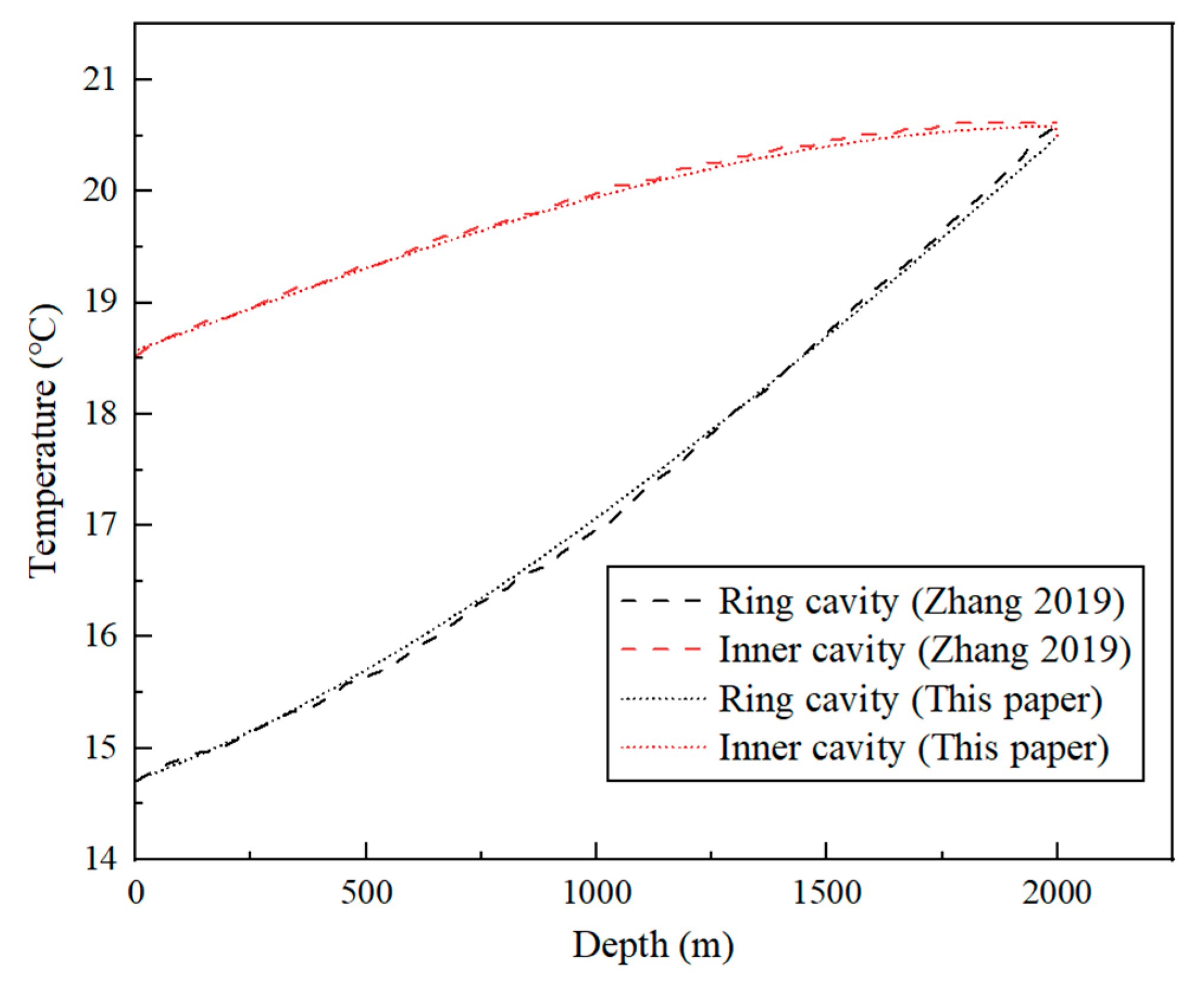
2.3. Model Validation

In order to validate the model, the results of the model were compared with the results obtained by Reference [3]. As shown in Figure 4, a comparison was made under the condition of the inlet temperature of 14.72 °C and a flow rate of 12 kg/s.

It can be seen from the figure that the simulation results of the model in this paper have similar temperature distribution curves with the results in the literature. The change trends of the two curves are also consistent. Although the results are not exactly the same, the differences are within an acceptable range. Therefore, it is considered that the model has a sufficiently high accuracy for subsequent research.

2.4. Heat Pump Model

The power consumption of the heat pump was calculated using the Gordan model [34]. Although the Gordan model is a semi-empirical one for the refrigerator established by theoretical thermodynamic analysis and experiments, it can also be applied to the calculation of the heat pump power consumption, which is calculated using the following equation:

$$P_{hp}={\mathrm{Q}}_{\mathrm{F}}\left[\left(L_{\mathrm{d}}+{\mathrm{C}}_1\right)\frac{T_{\mathrm{c},\mathrm{in}}}{T_{\mathrm{e},\mathrm{out}}}-\mathrm{K}\left(L_{\mathrm{d}}+{\mathrm{C}}_2\right)\right]$$

(8)

where ${\mathrm{Q}}_{\mathrm{F}}$ is the heating capacity at a full load under a rated operating condition, kW. $L_{\mathrm{d}}$ is the load rate, %. $T_{\mathrm{c},\mathrm{in}}$ is the inlet temperature of condenser, K. $T_{\mathrm{e},\mathrm{out}}$ is the outlet temperature of the evaporator, K. ${\mathrm{C}}_1$, ${\mathrm{C}}_2$, and $\mathrm{K}$ are undetermined constants.

According to the parameters of the selected heat pump, the undetermined constant in Equation (9) is determined by fitting:

$$P_{hp}={\mathrm{Q}}_{\mathrm{F}}\left[\left(L_{\mathrm{d}}+0.669\right)\frac{T_{\mathrm{c},\mathrm{in}}}{T_{\mathrm{e},\mathrm{out}}}-1.003L_{\mathrm{d}}-0.653\right]$$

(9)

2.5. Heat Storage Tank Model

The heat storage power or heat release power of the heat storage tank can be calculated using the following equation:

$$P_{\mathrm{TES}}=\frac{\rho c_p\Delta T{q}_T}{3600}$$

(10)

where $P_{\mathrm{TES}}$ is the heat storage power or heat release power of the heat storage tank, kW. $\rho$ is the density of the hot water in the heat storage tank, kg·m⁻³. $c_p$ is the constant pressure-specific heat capacity of the hot water in the heat storage tank, J·kg⁻¹·K⁻¹. $\Delta T$ is the temperature difference between the inlet and outlet hot water of the heat storage tank, K. $q_T$ is the inlet and outlet flow rate of the heat storage tank, m³·h⁻¹.

2.6. Water Pump Model

Because the flow rate of each circulation step in the system varies with time, the variable frequency pump was applied and the power consumption was calculated using the following equation:

$$P_{wp}=\frac{\rho gqH}{3.6\times {10}^6\eta }$$

(11)

where $q$ is the flow rate of the circulating water pump, m³·h⁻¹. $H$ is the head of the circulating water pump, m. $\eta$ is the efficiency of the variable frequency pump.

The head is calculated according to the law of similarity:

$$\frac{q}{q_0}=\frac{n}{n_0}=k$$

(12)

$$\frac{H}{H_0}={\left(\frac{n}{n_0}\right)}^2=k^2$$

(13)

where $q_0$ is the rated flow rate of the variable frequency pump, m³·h⁻¹. $H_0$ is the rated head of the variable frequency pump, m. $n_0$ and $n$ are the rated and actual speed of the variable frequency pump, respectively, r·min⁻¹. $k$ is the speed ratio.

The efficiency $\eta$ consists of three parts: the pump efficiency ${\eta }_{\mathrm{p}}$, the motor efficiency ${\eta }_{\mathrm{e}}$, and the inverter efficiency ${\eta }_{\mathrm{t}}$:

$$\eta ={\eta }_{\mathrm{p}}{\eta }_{\mathrm{e}}{\eta }_{\mathrm{t}}$$

(14)

The three are calculated according to the empirical equations [35]:

$${\eta }_{\mathrm{p}}={\eta }_{\mathrm{p}0}\sin \left(k\cdot \frac{\mathsf{\pi }}{2}\right)$$

(15)

$${\eta }_{\mathrm{e}}=0.94187\left[1-\exp \left(-9.04k\right)\right]$$

(16)

$${\eta }_{\mathrm{t}}=0.5067+1.283k-1.42k^2+0.5842k^3$$

(17)

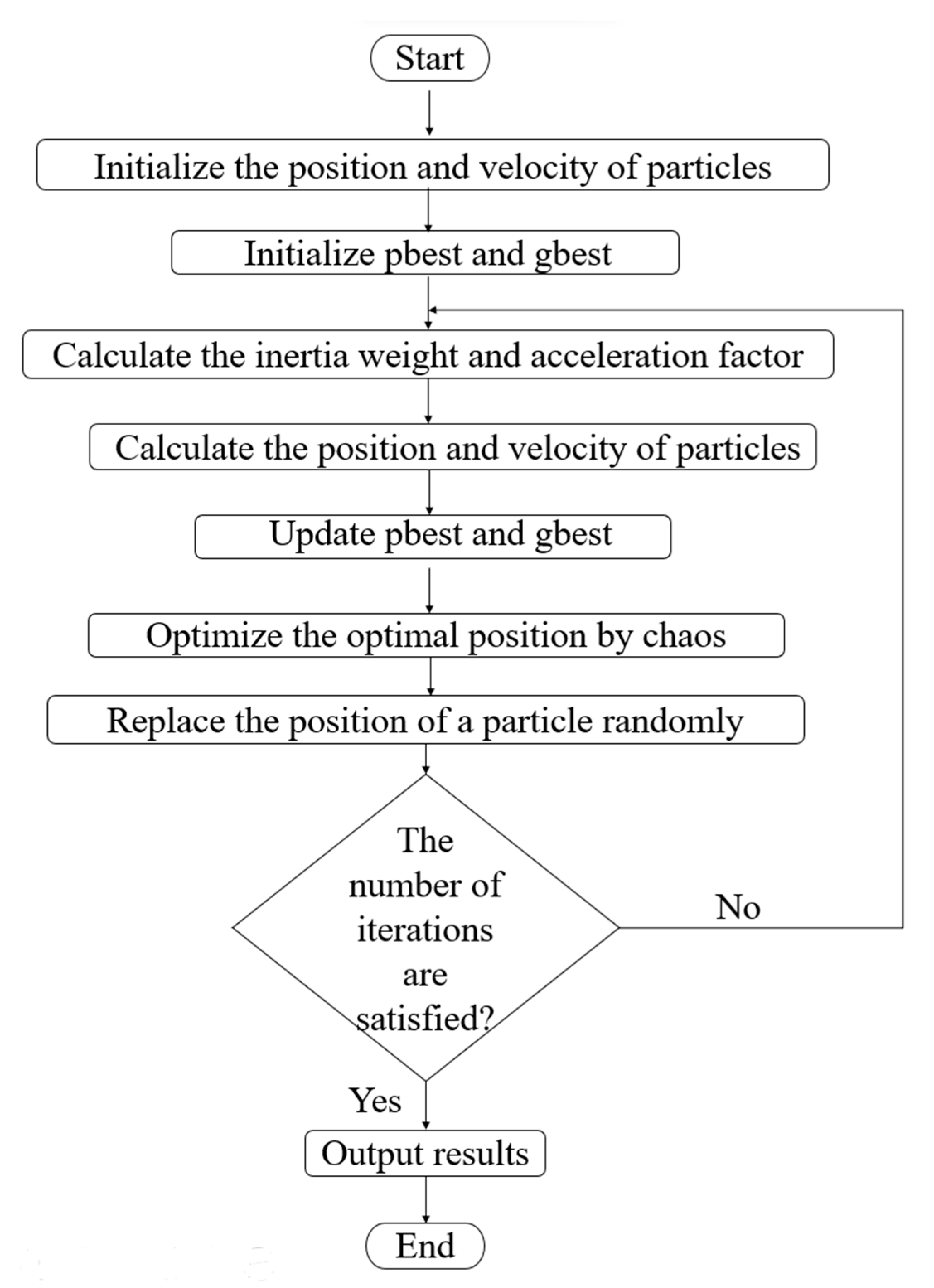
3. Improvement of Particle Swarm Optimization Algorithm

3.1. Particle Swarm Algorithm Model

The particle swarm algorithm (PSO) is a swarm intelligence algorithm designed by simulating the feeding behavior of birds [36]. In nature, birds are continuously searching and exchanging information in a region to find food. Similarly, the particle swarm algorithm randomly generates a group of particles in the search space so that the particles are all evaluated by a fitness value (Fitness) determined by the objective function and have a certain speed, thus they are moving continuously in the space. In each iteration, the individual optimal value pbest and the group optimal value gbest were obtained by comparing the fitness values of each particle. The velocity and position of the particles were updated by Equations (18) and (19) based on the positions of pbest and gbest.

$$v_{id}^{\left(k\right)}=\omega v_{id}^{\left(k-1\right)}+c_1{r}_1\left(pbes{t}_{id}-x_{id}^{\left(k-1\right)}\right)+c_2{r}_2\left(gbes{t}_d-x_{id}^{\left(k-1\right)}\right)$$

(18)

$$x_{id}^{\left(k\right)}=x_{id}^{\left(k-1\right)}+v_{id}^{\left(k\right)}$$

(19)

where $\omega$ is the inertia weight. $c_1$, $c_2$ are the accelerating factors. $r_1$, $r_2$ are the independent random variables which are uniformly distributed throughout [0, 1].

3.2. Improvement of the Particle Swarm Algorithm

The particle swarm algorithm suffers from the problem of a premature convergence and tends to fall into local optimality for the multimodal function as the objective function. In order to solve this problem, researchers have proposed numerous different improvement schemes in which one idea is applied to adjust the parameter settings of the algorithm. In the particle swarm algorithm, the parameter settings of the inertia weight $\omega$ and the accelerating factors $c_1$ and $c_2$ have an important influence on the performance of the algorithm. The global search ability of the algorithm can be improved by increasing the value of $\omega$; otherwise, the local search ability can be enhanced. Because the $c_1$ and $c_2$ represent the individual cognition and group cognition of the particles, respectively, the algorithm has a better local search ability when $c_1$ is smaller and $c_2$ is larger; otherwise, the global search ability is better. In order to avoid a premature convergence, the global search ability should be enhanced in the early iterations, while the local search ability should be enhanced in the late iterations. Therefore, $\omega$ decreases by the law of cosine function in the process of iteration, while $c_1$ and $c_2$ decrease and increase linearly, respectively, as shown in Equations (20)–(22):

$$\omega ={\omega }_{\min }+\cos \left(\frac{i-1}{i_{\max }-1}\right)\cdot \left({\omega }_{\max }-{\omega }_{\min }\right)$$

(20)

$$c_1=c_{1\mathrm{s}}+\frac{i-1}{i_{\max }-1}\cdot \left(c_{1\mathrm{e}}-c_{1\mathrm{s}}\right)$$

(21)

$$c_2=c_{2\mathrm{s}}+\frac{i-1}{i_{\max }-1}\cdot \left(c_{2\mathrm{e}}-c_{2\mathrm{s}}\right)$$

(22)

where ${\omega }_{\max }$, ${\omega }_{\min }$ are the upper and lower limits of the inertia weights, respectively. $c_{1\mathrm{s}}$, $c_{2\mathrm{s}}$ are the initial and final values of the acceleration factor $c_1$, respectively. $c_{2\mathrm{s}}$, $c_{2\mathrm{e}}$ are the starting and final values of the acceleration factor $c_2$, respectively. $i$ is the current number of iterations. $i_{\max }$ is the maximum number of iterations.

In addition, researchers have proposed some improved hybrid particle swarm algorithms by referring to ideas from other optimization algorithms. For example, the idea of chaos optimization can be introduced into the particle swarm algorithm, which improves to the chaotic particle swarm optimization algorithm (CPSO) [37]. On the one hand, the position and velocity of the particles were initialized by the chaotic sequence; on the other hand, the chaotic sequence was generated based on the optimal position of the group, while one particle in the current particle swarm was randomly replaced by the optimal particle.

Herein, the logistic equation was applied to the chaotic system in the optimization:

$$z_{n+1}=\mu z_n\left(1-z_n\right),n=0,1,2,\cdots ,Z_{n+1}$$

(23)

where $\mu$ is the control parameter, $\mu =4$, and the initial value $z_0$ satisfies $0\le z_0\le 1$.

The algorithmic flow of the improved particle swarm optimization algorithm applied is shown in Figure 5:

3.3. Objective Function

Herein, January 15 was chosen as a typical day for research, and the circulation flow rate in the buried pipe was applied to the optimal decision variable.

It can evaluate the medium-depth GSHP system from multiple perspectives, including economy, energy efficiency, as well as clean energy utilization. Therefore, three objective functions were designed to optimize the system, including operating costs, system COP, and the geothermal energy utilization coefficient.

The operating cost is the sum of the electricity cost generated by the system operation in each hour:

$$\min w={{\displaystyle \sum }}_{t=1}^{24}\left(P_{\mathrm{hp}}\left(t\right)+P_{\mathrm{wp}}\left(t\right)\right)\cdot \Delta t\cdot e\left(t\right)$$

(24)

where $P_{\mathrm{hp}}\left(t\right)$ is the heat pump power consumption of $t$ period, kW. $P_{\mathrm{wp}}\left(t\right)$ is the pump power consumption of $t$ period, kW, and $e\left(t\right)$ is the electricity price of $t$ period, RMB Yuan·kWh⁻¹.

The system COP is defined as the ratio of the system’s heat supply to the system’s power consumption:

$$\max CO{P}_{\mathrm{s}}=\frac{{{\displaystyle \sum }}_{t=1}^{24}\left(P_{\mathrm{geo}}\left(t\right)+P_{\mathrm{hp}}\left(t\right)+P_{\mathrm{wp},\mathrm{h}}\left(t\right)\right)}{{{\displaystyle \sum }}_{t=1}^{24}\left(P_{\mathrm{hp}}\left(t\right)+P_{\mathrm{wp}}\left(t\right)\right)}$$

(25)

where $P_{\mathrm{geo}}\left(t\right)$ is the heat extraction of the buried pipes in $t$ period, kW. $P_{\mathrm{wp},\mathrm{h}}\left(t\right)$ is the power consumption of the ground source side pump in $t$ period, kW.

The geothermal energy utilization coefficient was defined as the ratio of the heat extraction of the buried pipes to the heat supply of the system:

$$\max \xi =\frac{{{\displaystyle \sum }}_{t=1}^{24}{P}_{\mathrm{geo}}\left(t\right)}{{{\displaystyle \sum }}_{t=1}^{24}\left(P_{\mathrm{geo}}\left(t\right)+P_{\mathrm{hp}}\left(t\right)+P_{\mathrm{wp},\mathrm{h}}\left(t\right)\right)}$$

(26)

3.4. Constraint Condition

Considering the actual situation of the system’s operation, the following constraints were set in the optimization:

①

Thermal power balance constraint.

Part of the heat supply of the system is applied to meet the user’s heat load, while the remainder is stored in the heat storage tank. If the calculated heat storage power is negative, then the storage tank is in a heat release state.

$$P_{\mathrm{geo}}\left(t\right)+P_{\mathrm{hp}}\left(t\right)+P_{\mathrm{wp},\mathrm{h}}\left(t\right)=P_{\mathrm{load}}\left(t\right)+P_{\mathrm{TES}}\left(t\right)$$

(27)

where $P_{\mathrm{load}}\left(t\right)$ is the heat load of users in $t$ period, kW. $P_{\mathrm{TES}}\left(t\right)$ is the heat storage power of the heat storage tank in $t$ period, kW.

②

Water pump flow rate constraint.

The flow rate of the water pump should be greater than the specified minimum flow rate, but it should not be more than its rated flow rate either:

$$Q_{\mathrm{TES},\min }\le Q_{\mathrm{TES}}\le Q_{\mathrm{TES},\max }$$

(28)

③

Heat storage capacity constraint.

The heat energy stored in the heat storage tank cannot exceed its heat storage capacity, and it cannot be lower than the specified minimum value:

$$E_{\mathrm{TES},\min }\le E_{\mathrm{TES}}\le E_{\mathrm{TES},\max }$$

(29)

4. Results and Discussion

4.1. Operating Costs as the Objective Tunction

The optimization objective is to minimize the operating costs, in which the results obtained from the simulations are shown in Figure 6, Figure 7 and Figure 8.

As can be seen from Figure 6, the buried pipe flow rate first decreases from approximately 14 m³/h to 8.5 m³/h and then increases to 11 m³/h, with 18:00 as the demarcation point. Additionally, the buried pipe flow rate is high when the electricity price is low, while it is low when the electricity price is high.

Figure 7 depicts the heat storage capacity and consumers’ heat load of each period after optimization. According to the profile of the heat storage with time, the working conditions of the heat storage tank can be mainly divided into three stages: 2:00–10:00 and 20:00–24:00 are both the heat release stage, while 12:00–20:00 is the heat storage stage. The heat storage capacity first changes from approximately 300 kW to 0 in 2:00–10:00, then from 0 to 150 kW in 12:00–20:00, and then to 0 in 20:00–24:00. Compared with the profile of the heat load, the heat load is smaller during the heat storage period and basically at a high level during the heat release period. In contrast, compared with the time-of-use electricity price curve, the heat storage period is basically the valley electricity period, but the heat release period is basically the peak electricity period. Therefore, it can be assumed that the operating mode of the heat storage tank at this time is jointly determined by the consumers’ heat load and the electricity price.

Figure 8 illustrates the power consumption of each period after optimization; it can be seen that the variation in the heat pump power consumption is very small and the variation trend in the total power consumption is mainly determined by the water pump power consumption. It can be seen from Figure 7 that 21:00–10:00 is the higher power consumption period of the system, which is mainly due to the larger flow rate of the buried pipe at this time, resulting in the higher power consumption of the pump on the ground source side. Overall, the system is designed to reduce operating costs by increasing the heat supply and storing heat during the valley electricity period as well as releasing heat during the peak electricity period, thereby shifting the power consumption of the system over time.

4.2. System COP as the Objective Function

Taking the optimization objective as the highest system COP, the simulation results are shown in Figure 9, Figure 10 and Figure 11.

Figure 9 illustrates the flow rate in buried pipes in each period after optimization, from which it can be seen that the flow rate in buried pipes fluctuates constantly, but always maintains a high level, with a maximum of 14 m³/h and a minimum of 11.75 m³/h.

Figure 10 compares the heat storage and the consumers’ heat load of each period after optimization. It can be seen that the variation trend in the heat storage is basically decreasing first and then increasing as time goes by. Therefore, the working conditions of the heat storage tank are mainly divided into two stages: 1:00–10:00 is the heat release stage, and 10:00–20:00 is the heat storage stage. The heat storage capacity first changes from approximately 250 kW to 0 in 1:00–10:00, and then from 0 to approximately 460 kW in 10:00–20:00. While the heat load of the consumers at 1:00–10:00 is larger and increasing, while the heat load at 10:00–20:00 is small and decreasing, which means that the working modes of the heat storage tank are determined by the heat load of the consumers at this time.

Figure 11 shows the power consumption of each period after optimization. It can be seen that the power consumption of the heat pump changes very little and the total power consumption and water pump power consumption fluctuate within a small range. Therefore, in order to obtain a high system COP, the buried pipe flow rate should be maintained at a high level, and the heat storage tank should store or release heat according to the user’s heat load.

4.3. Geothermal Energy Utilization Coefficient as the Objective Function

Taking the optimization objective as the maximum geothermal energy utilization coefficient, the results obtained from the simulation are shown in Figure 12, Figure 13 and Figure 14. It can be seen that the results obtained are close to those when the objective function is the system COP, which indicates that the optimization effects with the system COP and the geothermal energy utilization coefficient as the objective function are similar.

4.4. Improvement of the Particle Swarm Algorithm

Table 2. Evaluation indicators of the system after optimization with different objective functions.

Objective Functions	Operating Costs (CNY)	System COP	Geothermal Energy Utilization Coefficient
Operating costs	279.27	5.8257	0.8369
System COP	300.02	6.4420	0.8524
Geothermal energy Utilization coefficient	300.74	6.4413	0.8527

lists the evaluation indices for the system after optimization with different objective functions. It can be seen that the variation trend in the operating costs and the system COP are opposite, with one reaching the optimum and the other reaching the worst. The variation trend in the geothermal energy utilization coefficient is the same as the system COP, but its range is limited.

5. Conclusions

In this study, a medium-depth GSHP system is fabricated for an office building in Xi’an, in which the particle swarm algorithm is improved by adjusting the parameters of the algorithm and introducing the chaotic optimization idea. Based on the improved particle swarm optimization algorithm, the system operation is optimized with the operating costs, system COP, and the geothermal energy utilization coefficient as the objective functions, respectively, while the optimization results are compared and analyzed. The main conclusions are as follows:

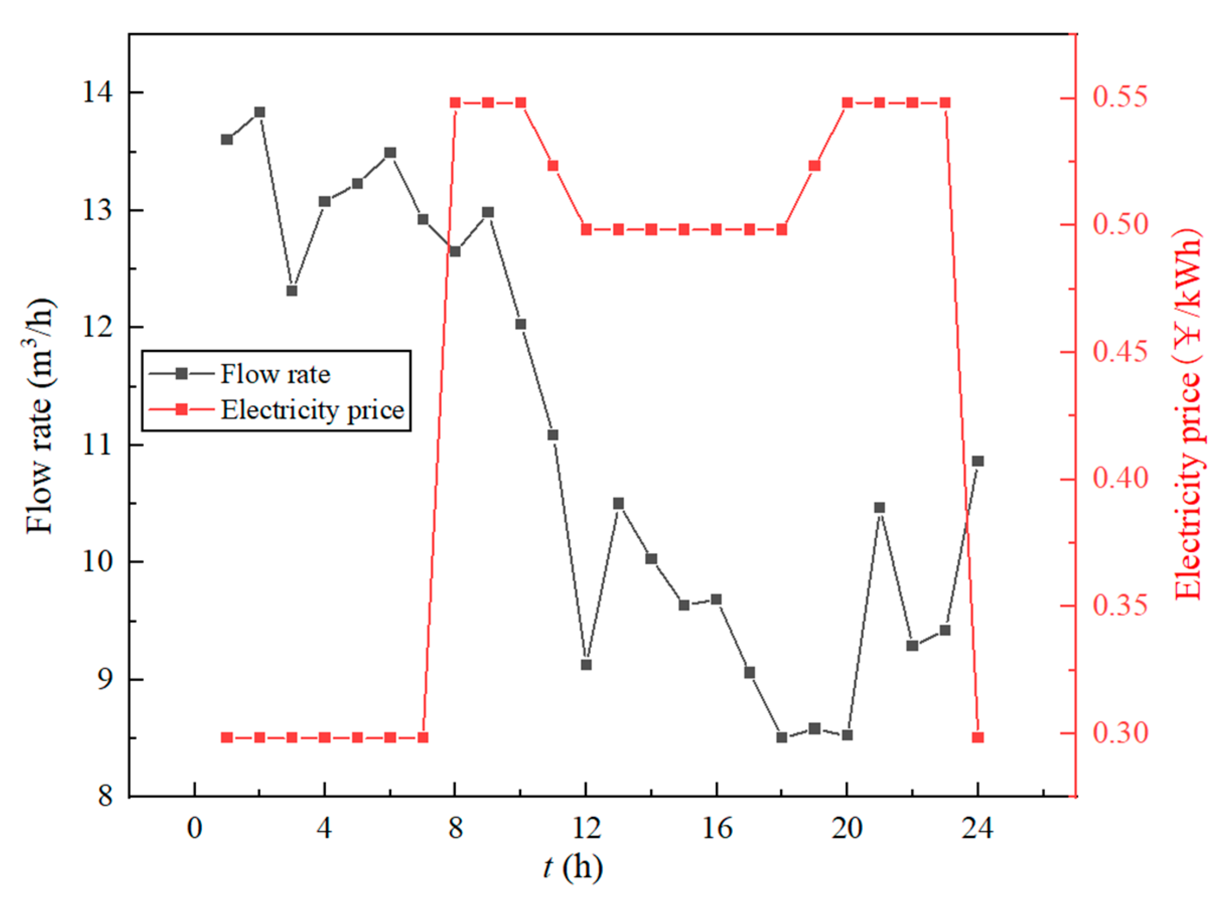
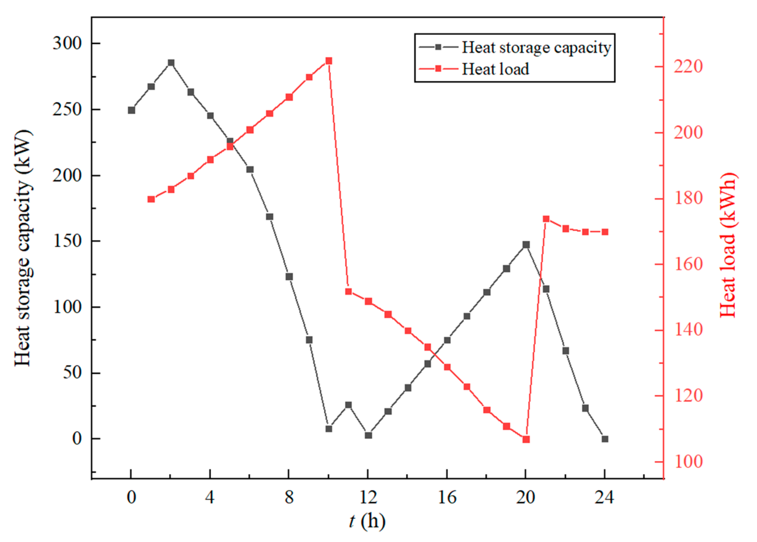
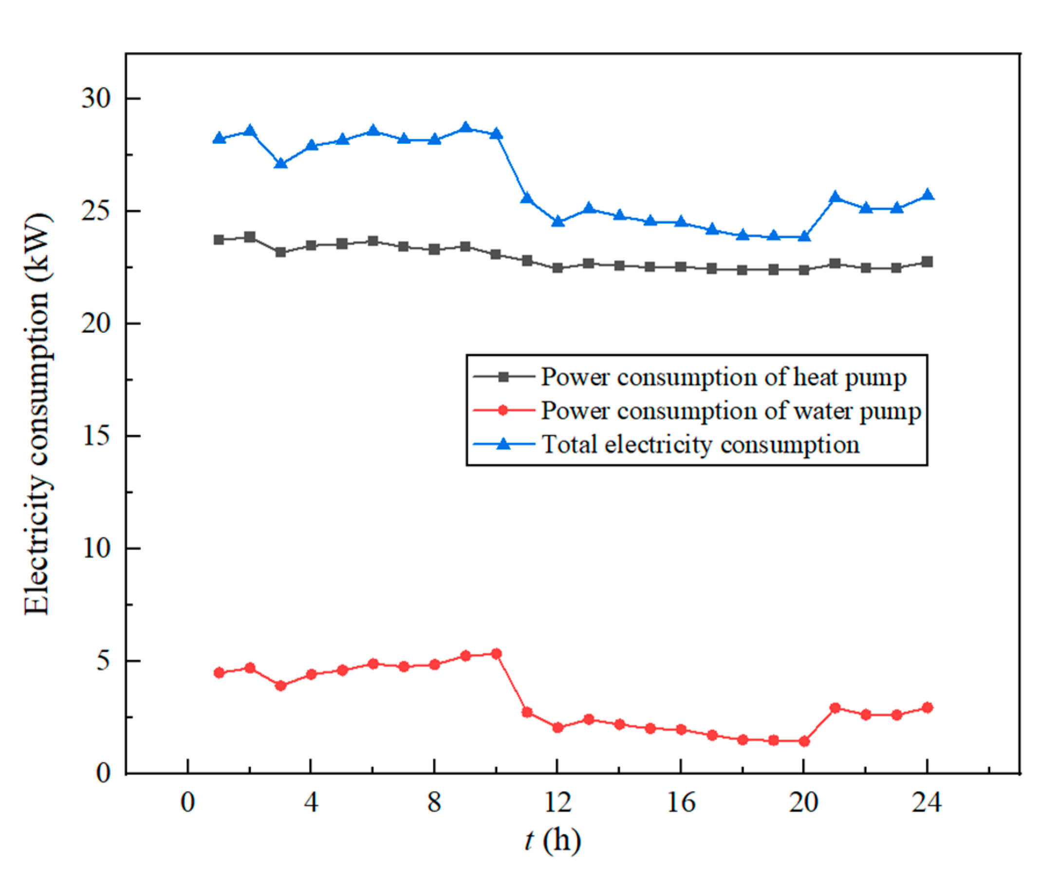
• Taking the operating costs as the objective function, the buried pipe flow rate first decreases from approximately 14 m³/h to 8.5 m³/h and then increases to 11 m³/h with 18:00 as the demarcation point, and the higher power consumption of the system in 21:00–10:00, about 25–30 kW. At the same time, the working conditions of the heat storage tank are mainly divided into three stages, 2:00–10:00, 20:00–24:00, which is the heat release mode, and 12:00–20:00, which is the heat storage mode. The heat storage capacity first changes from approximately 300 kW to 0 in 2:00–10:00, then from 0 to 150 kW in 20:00–24:00, and then to 0 in 12:00–20:00. Furthermore, the system transfers some of the power consumption from the peak power period to the valley power period by switching the heat storage and heat release modes of the heat storage tank. In this way, the operating cost is the lowest, CNY 279.27. The system COP and the geothermal energy utilization coefficient are 5.8257 and 0.8369, respectively.
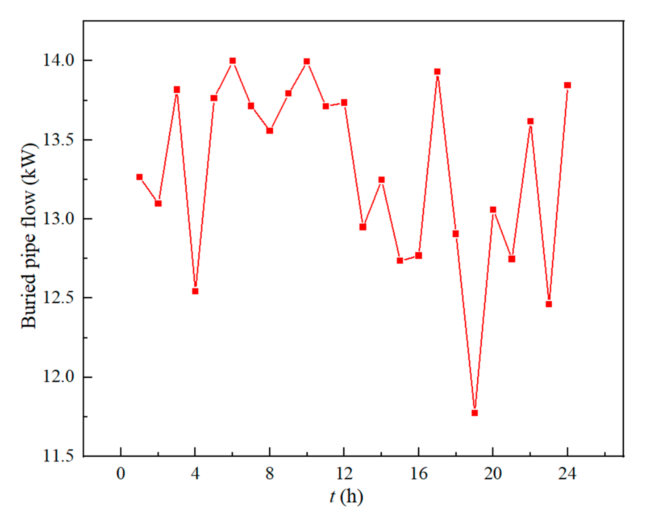
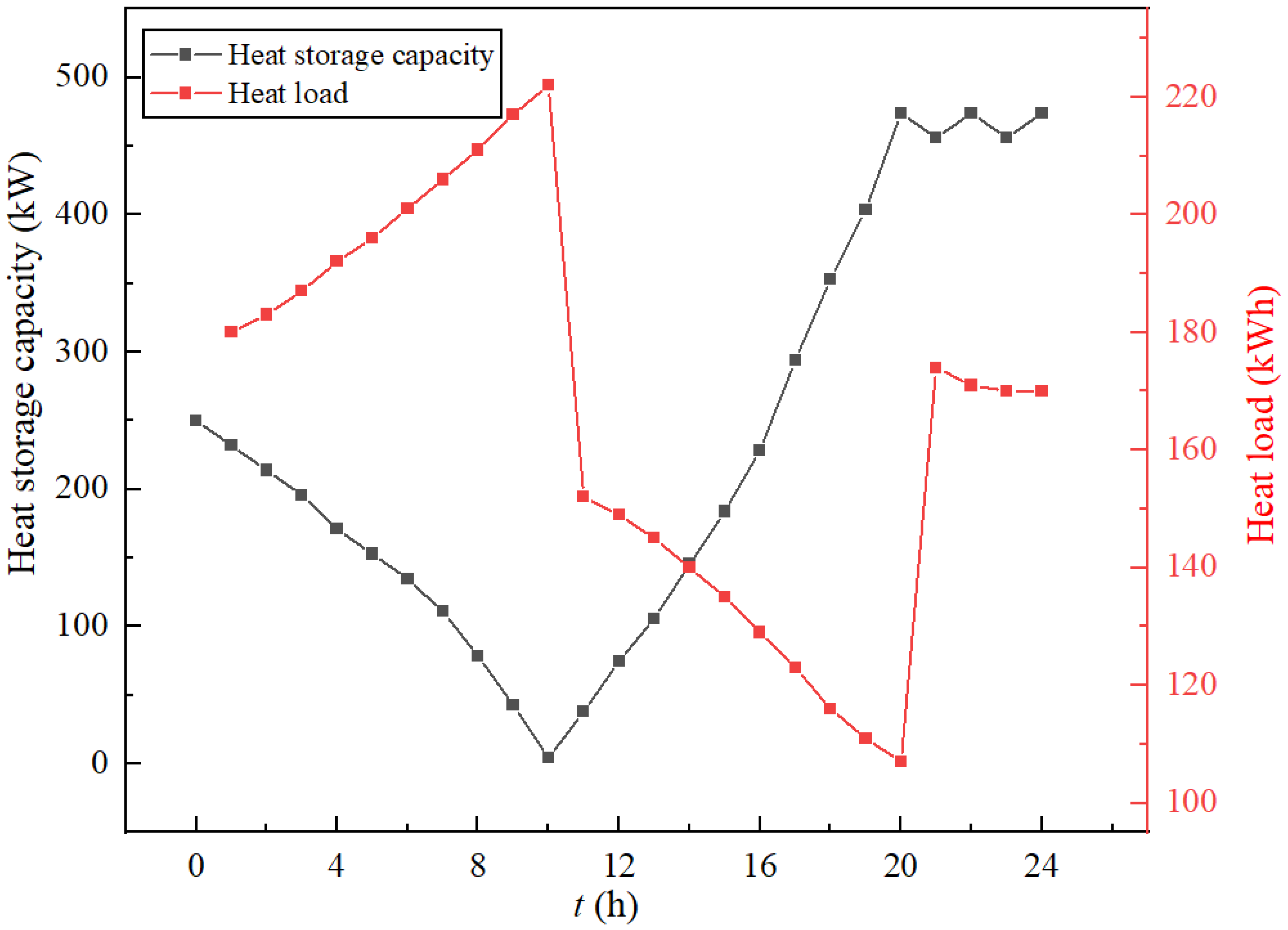
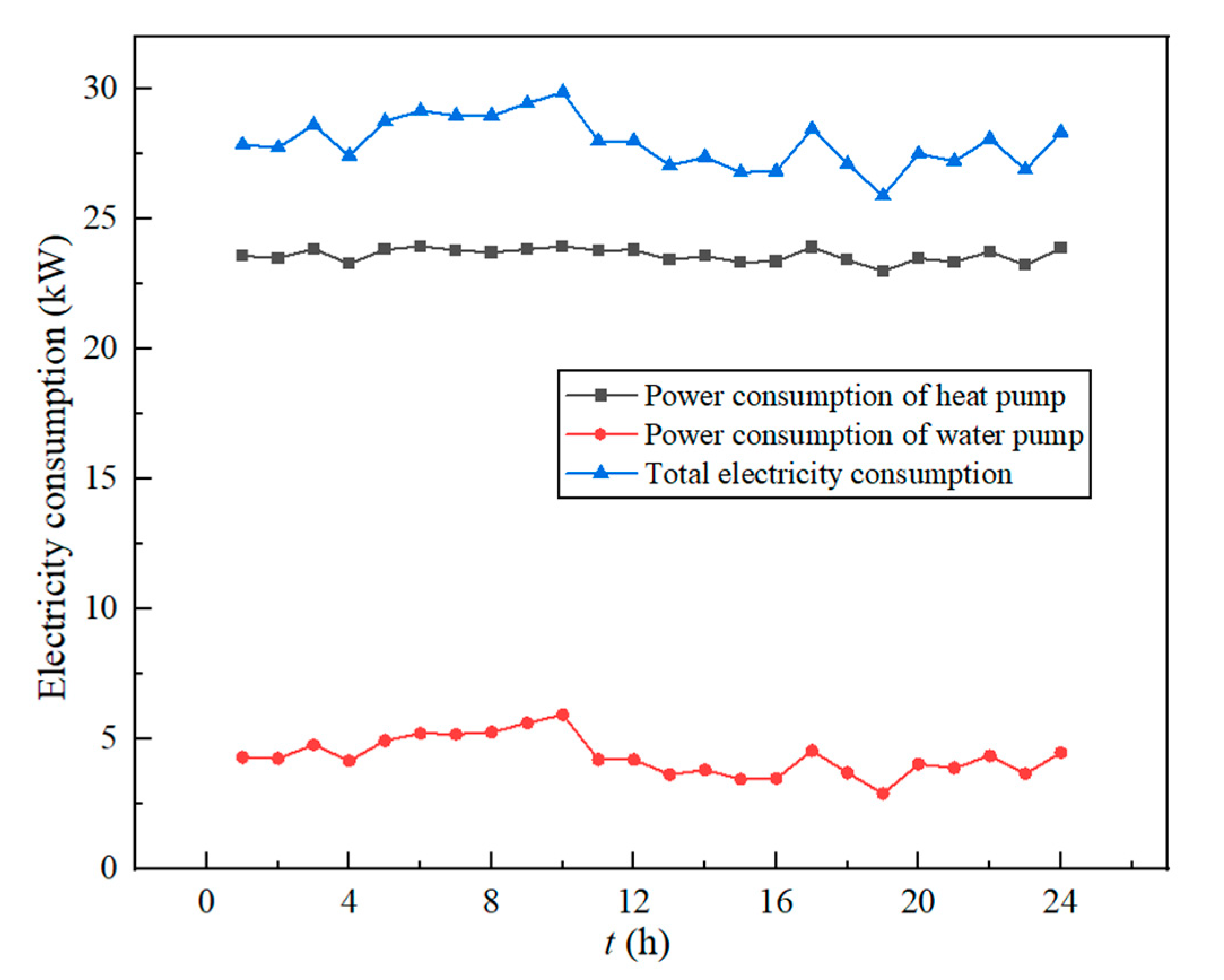
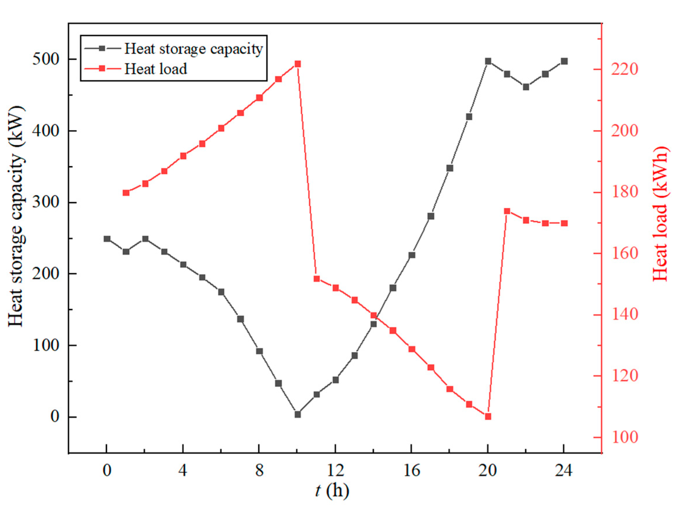
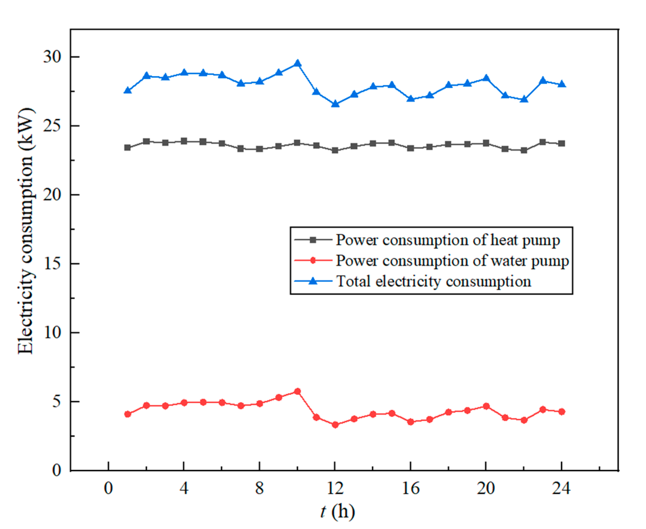
• Taking the system COP as the objective function, the buried pipe flow rate fluctuates slightly at a high level, with a maximum of 14 m³/h and a minimum of 11.75 m³/h. However, the system power consumption varies little with time, staying at around 27 kW. In this way, the working conditions of the heat storage tank are mainly divided into two stages: 1:00–10:00 is the heat release mode, and 10:00–20:00 is the thermal storage mode. The heat storage capacity first changes from approximately 250 kW to 0 in the 1:00–10:00 stage, and then from 0 to approximately 460 kW in the 10:00–20:00 stage. In addition, the heat supply of the system is maintained at a relatively stable level at all times by switching the heat storage and heat release modes of the heat storage tank. In this case, the maximum system COP is 6.4420. The operating cost and the geothermal energy utilization coefficient are 300.02 and 0.8524, respectively.
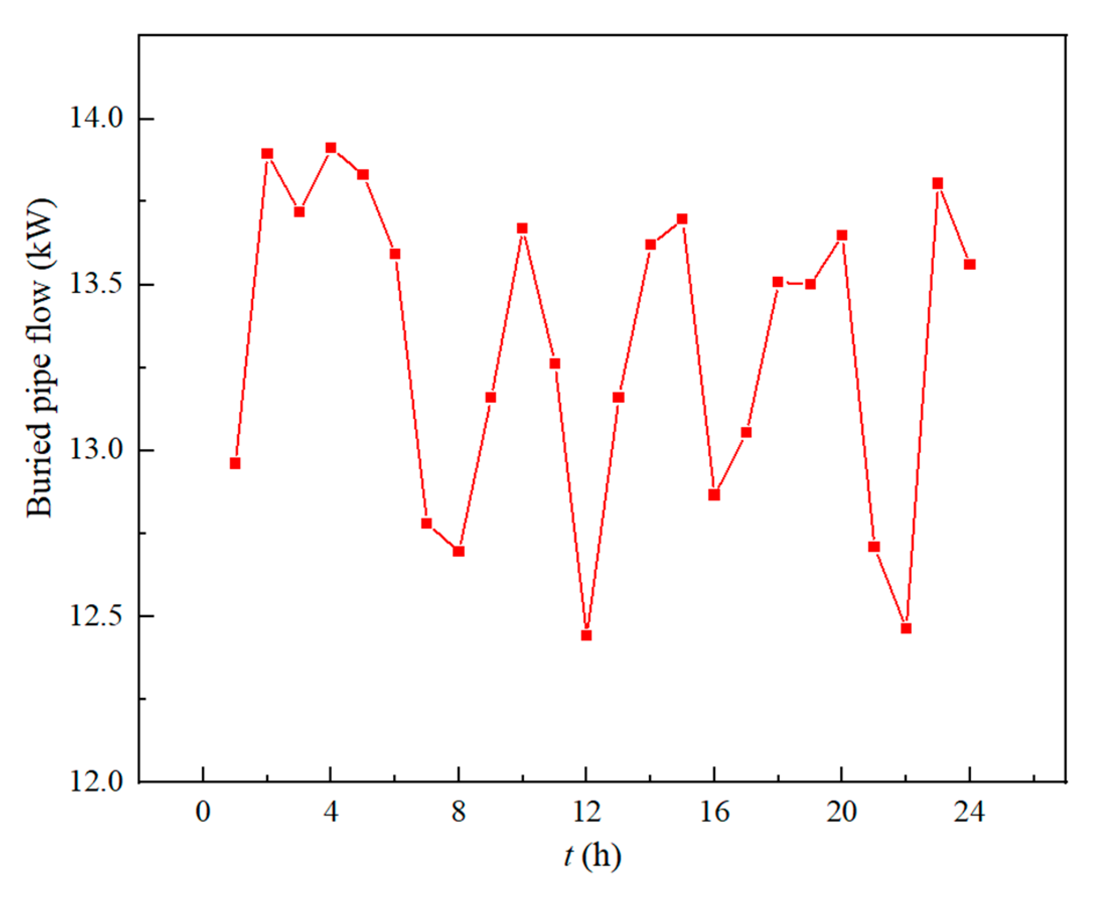
• Taking the geothermal energy utilization coefficient as the objective function, it can be seen that the optimization effects are similar to the effect of taking the system COP as the objective function. At this time, the maximum geothermal energy utilization coefficient is 0.8527. The operating cost and the system COP are 300.74 and 6.4413, respectively.
• Comparing the three objective functions, it can be revealed that the operating costs are opposite to the optimization effects of the system COP, while the values of the geothermal energy utilization coefficient are not much different under different objective functions.

References

1. Wang, F.H.; Cai, W.L.; Wang, M.; Gao, Y.; Liu, J.; Wang, Z.H.; Xu, H. Status and outlook for research on geothermal heating technology. J. Refrig. 2021, 42, 14–22. (In Chinese) [Google Scholar] [CrossRef]
2. Li, J.; Xu, W.; Li, J.F.; Li, Z.; Zhang, Y.Q.; Yang, C.; Qiao, B.; Sun, Z.Y.; Wang, X.; Xiao, L.; et al. Heat supply technology review and engineering measurement analysis of medium and deep buried pipes. HVAC 2020, 50, 35–39. (In Chinese) [Google Scholar]
3. Zhang, B.B. Study on Energy Efficiency of Medium-Depth Borehole Casing Type Buried Pipe Heat Exchanger and Ground Source Side Water System; Shandong Architecture University: Jinan, China, 2019. (In Chinese) [Google Scholar]
4. Ren, Y.Z. Experimental Study on Medium Medium-Depth Soil Source Heat Pump System in Severe Cold Area; Harbin Institute of Technology: Harbin, China, 2019. (In Chinese) [Google Scholar]
5. Deng, J.W.; Wei, Q.P.; Liang, M.; He, S.; Zhang, H. Field test on the energy performance of medium-depth geothermal heat pump systems (MD-GHPs). Energy Build. 2019, 184, 289–299. [Google Scholar] [CrossRef]
6. Pratiwi, A.S.; Trutnevyte, E. Life cycle assessment of shallow to medium-depth geothermal heating and cooling networks in the State of Geneva. Geothemics 2020, 90, 101988. [Google Scholar] [CrossRef]
7. Zuo, T.T.; Li, X.L.; Wang, Z.S. Application of medium-depth double U-tube ground-source heat pump systems to severe cold zone. HVAC 2021, 51, 118–123. (In Chinese) [Google Scholar]
8. Wang, W. Optimization analysis of the operation strategy of medium and deep ground source heat pump heating system. Build. Energy Build. 2022, 41, 62–67. (In Chinese) [Google Scholar]
9. Du, S.S. Design load ratio analysis of medium and deep ground source heat pump heating system with auxiliary heat source in northwest China. Northwest. Hydropower 2022, 1, 95–98+102. (In Chinese) [Google Scholar]
10. Ma, J.X.; Zhang, X.G.; Yao, X.Y.; Li, Y. Design and application of medium-depth geothermal heating system in a residential district of Xianyang. HVAC, 2022; 52, 200–204. (In Chinese) [Google Scholar]
11. Wang, X.Y.; Zhou, C.H.; Ni, L. Experimental investigation on heat extraction performance of deep borehole heat exchanger for ground source heat pump systems in severe cold region. Geothemics 2022, 105, 102539. [Google Scholar] [CrossRef]
12. Guo, H.M.; Wu, J.H.; Hu, P.F.; Ren, H.J.; Zhang, J.; Li, Z.X. The measurement and analysis for a medium-depth geothermal heat pump system. China Min. Mag. 2023, 32, 165–172. (In Chinese) [Google Scholar]
13. Zhao, B.; Guo, C.X.; Cao, Y.J. An improved particle swarm optimization algorithm for optimal reactive power dispatch. In Proceedings of the 2005 IEEE Power Engineering Society General Meeting, San Francisco, CA, USA, 12–16 June 2005; pp. 272–279. [Google Scholar]
14. Mussetta, M.; Selleri, S.; Pirinoli, P.; Zich, R.E.; Matekovits, L. Improved particle swarm optimization algorithms for electromagnetic optimization. J. Intell. Fuzzy Syst. Appl. Eng. Technol. 2008, 19, 75–84. [Google Scholar]
15. Zhang, R.; Zhang, Q.; Wang, B. Improved particle swarm optimization algorithm for designing DNA codewords. Inf.-Int. Interdiscip. J. 2009, 12, 497–505. [Google Scholar]
16. Gu, W.; Li, X.Y.; Wang, Y.H. Design of subsynchronous damping control based on improved particle swarm optimization algorithm by STATCOM. In Proceedings of the 2010 Asia-Pacific Power and Energy Engineering Conference (APPEEC), Chengdu, China, 28–31 March 2010; pp. 2903–2906. [Google Scholar]
17. Liu, N.P.; Zheng, F.; Xia, K.W. CDMA multiuser detection based on improved particle swarm optimization algorithm. In Proceedings of the International Conference on Intelligent Structure and Vibration Control (ISVC 2011), Chongqing, China, 14–16 January 2011; Volume 50–51, pp. 3–7. [Google Scholar]
18. Ma, X. Optimal operation of hydropower station based on improved particle swarm optimization algorithm. In Proceedings of the International Conference on Advanced Research on Computer Science and Information Engineering, Zhengzhou, China, 21–22 May 2011; Volume 153, pp. 226–231. [Google Scholar]
19. Kumar, N.; Nangia, U.; Sahay, K.B. Economic load dispatch using improved particle swarm optimization algorithms. In Proceedings of the 6th IEEE Power India International Conference (PIICON), Delhi, India, 5–7 December 2014; pp. 1–6. [Google Scholar]
20. Cao, H.Q.; Xu, J.; Ke, D.P.; Jin, C.X.; Deng, S.C.; Tang, C.H.; Cui, M.J.; Liu, J. Economic dispatch of micro-grid based on improved particle-swarm optimization algorithm. In Proceedings of the 48th North American Power Symposium (NAPS), Denver, CO, USA, 18–20 September 2016. [Google Scholar]
21. Song, Z.K.; Wang, P.; Bai, L.Q. Optimization of pulse CVT based on improved particle swarm algorithm. In Proceedings of the 2nd International Conference on Materials Science, Machinery and Energy Engineering (MSMEE 2017), Dalian, China, 13–14 May 2017; Atlantis Press: Dordrecht, The Netherlands; Volume 123, pp. 835–839. [Google Scholar]
22. Luo, Y.Q.; Zeng, B. An intelligent scheduling method based on improved particle swarm optimization algorithm for drainage pipe network. AIP Conf. Proc. 2017, 1864, 020037. [Google Scholar]
23. Luo, K.Y. Power system fault harmonic analysis based on improved particle swarm optimization algorithm. AIP Conf. Proc. 2019, 2066, 020015. [Google Scholar]
24. Wang, W.; Peng, C.; Mi, H.Y.; Chen, C.L.; Zeng, D.L. Furnace flame recognition based on improved particle swarm optimization algorithm. Proc. Inst. Mech. Eng. Part I-J. Syst. Control. Eng. 2020, 234, 888–899. [Google Scholar] [CrossRef]
25. Ahmadi, S.; Sahnesaraie, M.A.; Talami, S.H.; Dini, F.; Zanganeh, M.M.; Ashgevari, Y. Determine the optimal switching angles symmetrical cascaded multilevel inverter using Improved particle swarm optimization algorithm. In Proceedings of the 18th IEEE World Symposium on Applied Machine Intelligence and Informatics (SAMI 2020), Herlany, Slovakia, 23–25 January 2020; pp. 329–335. [Google Scholar]
26. Tao, Q.Y.; Sang, H.Y.; Guo, H.W.; Wang, P. Improved particle swarm optimization algorithm for AGV path planning. IEEE Access 2021, 9, 33522–33531. [Google Scholar]
27. Cai, M.Z. Dormitory allocation method oriented to heuristic particle swarm genetic algorithm. In Proceedings of the 2nd International Conference on Artificial Intelligence and Information Systems (ICAIIS ’21), Chongqing, China, 28–30 May 2021; p. 51. [Google Scholar]
28. Feng, K.T.; Li, X.Y.; Qian, X.; Wu, L.H.; Zheng, H.; Chen, M.; Li, M.R.; Liu, B. Atmospheric optical turbulence profile model fitting based on improved particle swarm algorithm. Laser Optoelectron. Prog. 2022, 59, 0501002. (In Chinese) [Google Scholar]
29. Ioakimidis, C.S.; Thomas, D.; Rycerski, P.; Genikomsakis, K.N. Peak shaving and valley filling of power consumption profile in non-residential buildings using an electric vehicle parking lot. Energy 2018, 148, 148–158. [Google Scholar] [CrossRef]
30. Fang, C.; Xu, Q.; Wang, S.; Ruan, Y. Operation optimization of heat pump in compound heating system. Energy Procedia 2018, 152, 45–50. [Google Scholar] [CrossRef]
31. Bandyopadhyay, A.; Leibowicz, B.D.; Beagle, E.A.; Webber, M.E. As one falls, another rises? Residential peak load reduction through electricity rate structures. Sustain. Cities Soc. 2020, 60, 102191. [Google Scholar] [CrossRef]
32. Nouri, G.; Noorollahi, Y.; Yousefi, H. Designing and optimization of solar assisted ground source heat pump system to supply heating, cooling and hot water demands. Geothermics 2019, 82, 212–231. [Google Scholar] [CrossRef]
33. Diao, N.R. Buried Pipe Ground Source Heat Pump Technology; Higher Education Press: Beijing, China, 2006; pp. 21–22. (In Chinese) [Google Scholar]
34. Gordon, J.M.; Kim, C.N.; Hui, T.C. Centrifugal chillers: Thermodynamic modeling and a diagnostic case study. Int. J. Refrig. 1995, 18, 253–257. [Google Scholar] [CrossRef]
35. Bernier, B.M.A.; Bourret, B. Pumping energy and variable frequency drives. ASHRAE J. 1999, 41, 37–40. [Google Scholar]
36. Kennedy, J.; Eberhart, R. Particle swarm optimization. In Proceedings of the ICNN’95-International Conference on Neural Networks, Perth, WA, Australia, 27 November–1 December 1995; pp. 1942–1948. [Google Scholar]
37. Tang, X.L. The Theory and Application of Particle Swarm Optimization Algorithm Based on Chaos; Chongqing University: Chongqing, China, 2007. (In Chinese) [Google Scholar]
Figure 1. Schematic diagram of the medium-depth GSHP system (1—ground source side pump, 2—circulation pump, 3—heat storage pump, 4—heat release pump, 5—heat storage valve, 6—heating valve, 7 and 8—operating mode control valve.
Applsci 13 03821 g001
Figure 2. The building model in TRNSYS.
Applsci 13 03821 g002
Figure 3. Schematic diagram of the casing buried pipe heat exchanger (red arrows—fluid with high temperature; blue arrows—fluid with low temperature).
Applsci 13 03821 g003
Figure 4. Model validation [3].
Applsci 13 03821 g004
Figure 5. Flow chart of improved PSO algorithm.
Applsci 13 03821 g005
Figure 6. Buried pipe flow and electricity price in each period when the objective function is operating costs.
Applsci 13 03821 g006
Figure 7. Heat storage capacity and heating load in each period when the objective function is operating costs.
Applsci 13 03821 g007
Figure 8. Electricity consumption in each period when the objective function is operating costs.
Applsci 13 03821 g008
Figure 9. Buried pipe flow in each period when the objective function is system COP.
Applsci 13 03821 g009
Figure 10. Heat storage capacity and heating load in each period when the objective function is system COP.
Applsci 13 03821 g010
Figure 11. Electricity consumption in each period when the objective function is system COP.
Applsci 13 03821 g011
Figure 12. Buried pipe flow in each period when the objective function is geothermal energy utilization coefficient.
Applsci 13 03821 g012
Figure 13. Heat storage capacity and heating load in each period when the objective function is geothermal energy utilization coefficient.
Applsci 13 03821 g013
Figure 14. Electricity consumption in each period when the objective function is geothermal energy utilization coefficient.
Applsci 13 03821 g014