Estimation of Processing Times and Economic Feasibility of Producing Moringa oleifera Lam. Capsules in Mexico

Featured Application

The simulation of processes in the agricultural sector is necessary; this work studied a real production system. The results contributed to improving productivity in the processing of Moringa oleifera capsules, addressing an area of knowledge with limited research. This model can be used by new companies intending to invest in this area of agricultural products for human consumption. The results indicated that production is feasible at a commercial level.

Abstract

The production of Moringa oleifera capsules has emerged as a promising agricultural activity in Mexico, driven by the plant’s well-documented health and nutritional benefits. In response, farmers have begun producing Moringa oleifera as a dietary supplement, using artisanal methods with minimal production controls. This study aimed to estimate the processing times of the Moringa oleifera production system using simulation modeling with Arena^® software and to evaluate the economic feasibility of capsule production. Methodologically, it was approached as a case study in the state of Veracruz, and processing times were estimated through systematic sampling and modeled with Arena simulation software. Three simulation scenarios were considered to select a technically and economically viable alternative for agricultural producers, as follows: one with a 200-capsule encapsulator (1E200C), another with two 200-capsule encapsulators (2E200C), and a third with an 800-capsule encapsulator (1E800C). For the initial diagnosis, a research stay was conducted for 180 days, and the production capacity was set at 24,000 capsules due to raw material limitations. Results indicated that the 1E800C scenario reduced processing time by 60% compared to the 1E200C scenario and by 35% compared to the 2E200C scenario. Additionally, the 1E800C model required only Arena simulation software version 162 days (16 h) of work, while the 2E200C required 4 days (32 h) and the 1E200C required 7 days (56 h). In terms of production costs per unit of 90 capsules, the 1E200C was USD 3.93, the 2E200C was USD 3.64, and the 1E800C was USD 3.45. This study concluded that due to raw material limitations, the company can produce 12,800 units of 90 capsules per year. It is recommended to adopt the 1E800C encapsulator, which would lower the overall production costs by 12.23%, representing USD 0.48 per unit produced and resulting in an additional profit of USD 6150.50. Over a five-year evaluation period, the benefit–cost ratio was 5.03, the NPV was 922,370.11, and the IRR was 42.09%, indicating that this type of agribusiness in Mexico is both technically and economically feasible.

1. Introduction

In engineering sciences, simulation is used as a tool for decision-making at different scales, and its applications have generally been oriented toward manufacturing and services in the field of industrial engineering and quantitative methods for management to analyze a wide variety of systems and organizations [1,2]. A simulation model provides insight into the operation of a real system with the purpose of understanding the behavior of the business system [3]. Simulation has advantages that are relevant to existing systems, making it an effective tool for planning production systems [4], including reducing system development time, experimenting artificially with the system, and low development costs. The model can be used multiple times, it is easier to use than certain analytical techniques, it allows for controlled simulation, its development does not affect the real system, and it is useful in compressing the time of the company’s operation process [5].

1.1. Review of Empirical Evidence

Process simulation in empirical evidence has been applied in various scientific disciplines and is still in development [6]. Cases have been reported for modeling and analyzing the behavior of complex systems, understanding their dynamics, and predicting results [7,8]. Simulations of production lines in a factory Ref. [9] simulate workflow and resource allocation [10] to improve efficiency and productivity [11]. Furthermore, within the simulation of customer service systems, customer flow was analyzed in a service system environment. On the other hand, in the simulation of customer service systems, the flow of customers in a service system has been analyzed [12,13], as well as staffing strategies [14,15,16], waiting times [17,18], and resource distribution to optimize customer satisfaction [19,20]. Analyses have also been performed on logistics systems [21,22]. Another area that has been widely studied with simulation is vehicle flow systems in a transportation network [23,24,25], modeling traffic and intersections [26,27,28,29,30,31], and modeling public transportation systems [32,33,34,35,36], as well as health systems [37,38].

In the agricultural sector, models such as the Integrated Farm Systems Model DairyMod [39], DyNoFlo [40], SIMS (DAIRY) [41], and the Ruminant Farm Systems Model (RuFaS) [42] have been developed. Other dynamic models found in empirical evidence applied to livestock include Ruminant [43,44], LiveSim [45], CNCPS [46], Grazplan [47], and GLEAM [48]. Additionally, some agricultural system models reported are IMPACT-HHM [49,50,51], APSFARM [52], and FARMSIM [49,53].

In agriculture, Tensi et al. [54] used Monte Carlo simulation to evaluate the capacity of microbial applications to improve the sustainability of Dutch potato production. In aquaculture, the Energy Plus simulator was used as a building performance simulation (BPS) tool to model a fish farm with a focus on energy efficiency [55]. Another method called computational fluid dynamics (CFD) was used to simulate ammonia distribution on a livestock farm [56]. The finite element numerical approach with COMSOL Multiphysics software (Version 6.2) was used to simulate groundwater flow and salinity in a rice field adjacent to a marine shrimp farm [57].

To analyze systems with simulation, various software programs have been developed, including the Arena^® simulation developed by Rockwell Automation. This software allows researchers to create discrete event simulation models to study behavior over time and analyze different scenarios. The flexibility and detailed modeling capabilities of Arena^® make it suitable for a wide range of applications in engineering and system management [58].

1.2. Problem Statement

Although not all research has focused on the use of visual interface simulators for modeling and analysis, this work stands out in its relevance because the simulation of processes on small-scale agricultural farms is lacking in information and has received little attention. Limited studies have addressed solving problems associated with these agricultural production systems that seek to transform their products [37,59]. On the other hand, no evidence has been found for their modeling using discrete simulation with Arena in the agricultural sector. Therefore, this work addresses a knowledge gap in the agricultural sector, which is useful for farmers interested in generating value-added products, such as dietary supplements, to optimize manufacturing efficiency and make them financially feasible for development in this new normality. This is because the demand for products that help improve health is appreciated by consumers [60].

The problem addressed by this research focused on the 83% of small agro-industrial companies in which agricultural CEOs market dietary supplements made from Moringa oleifera leaves [61] and lack technical knowledge for product transformation using quantitative methods. Despite this, they embarked on capsule production and other products empirically, without any production control, with the aim of diversifying their income [62]. The driving force behind this research was the connection between academia and the company, which faced a greater demand for products when entering new markets and needed to increase its production capacity. Regarding its design, the processing facilities of its production system were divided into distant workstations, which resulted in low production process efficiency.

1.3. Justification and Relevance of the Research

The justification for this work involves the fact that Moringa oleifera has become popular in Mexico and around the world as a dietary supplement due to its nutritional properties [63,64,65,66,67]. Moringa oleifera is a tree native to the subtropical and tropical regions of South Asia, although it is also grown in other parts of the world due to its climatic adaptability [68]. Moringa oleifera leaves contain high levels of vitamins, minerals, antioxidants, and proteins, including iron, calcium, and potassium, as well as essential amino acids [69,70,71,72,73]; some studies have reported its bioactive components and health benefits [74].

In Mexico, plantations of Moringa oleifera are reported in five states and eleven municipalities, covering 428 hectares, with a yield of 1206 tons valued at USD 704,500, Michoacán is the main producer of Moringa oleifera, accounting for 98.7% of the total volume, with Huetamo being the municipality responsible for 98% of the national production [75]. In the state of Veracruz, there are no official data on commercial plantations of Moringa oleifera. Mota-Fernández et al. [76] reported plantations in the municipalities of Tierra Blanca, Soledad de Doblado, and Puerto de Veracruz, totaling less than 10 hectares. Their main purpose is to produce dietary supplements from the leaves, intending to offer Mexican consumers an alternative to complement their diet due to the health benefits it provides [62,77]. Recently, Carrión et al. [78] determined the agroecological potential of Moringa oleifera cultivation in the state of Veracruz, highlighting its high productive potential at the national level. Olson et al. [79] determined that Mexico has a wide extension of the ideal climate for its cultivation.

Moringa oleifera powder can be added to fortify food as a nutritional supplement due to its easy ingestion [80]. Therefore, the market for companies producing quality supplements is high, as the demand for dietary supplements is increasing. This is why the company BD Moringa^® was established, to offer a dietary supplement based on Moringa oleifera to this potential market due to the health benefits reported in the specialized literature [67,81]. Therefore, generating reliable and low-cost products will be essential to compete in this industry, which offers opportunities for farmers [74,82].

The relevance of this research lies in the underutilized uses of the parts of the Moringa oleifera tree; the seeds can be used for animal feed, soap and cosmetic production, insecticides, water treatment, coagulant, and oil, the root and bark are used for their nutritional properties in human food, and the leaves are used as fodder for farm animals and human consumption, as well as fertilizer [82]. The stems and shoots are used as livestock feed [83,84,85]. These aspects highlight the agro-industrial potential of Moringa oleifera as a business with a future, and their innovation and development need to be investigated more deeply at the enterprise level.

The social value of this work offers three aspects. Firstly, according to [86], there are 500 million small farmers worldwide cultivating less than five acres. To improve the lives of small farmers, it is essential to develop specific solutions for each market. In this context, processing their products through previous studies, modeling, and analyzing each stage of the manufacturing process of dietary supplements, from raw material reception to final product packaging, is feasible. Secondly, increasing sales makes this market more vulnerable to dishonest producers. Therefore, it is necessary to avoid safety and quality issues [87]. Finally, malnutrition is a widespread problem worldwide, affecting people of all backgrounds and ages [88]. Moringa oleifera leaf protein has been reported by nutritionists and consumers to treat nutritional deficiencies [89].

For these reasons, its practical implication is significant because simulating the production processes of dietary supplements in agricultural companies becomes a valuable tool for optimizing efficiency and process quality. By modeling and analyzing different scenarios, small agricultural entrepreneurs can make informed decisions to improve the productivity and profitability of their operations and projects without the need for large investments in new or existing systems.

The theoretical contribution of this work focuses on the engineering sciences in the fields of simulation, agronomy, and agricultural economics, complementing quantitative methods, economic engineering, and innovation in the context of the agro-industrial processing of Moringa oleifera, for which no similar studies exist. Therefore, the objectives of this work were, first, to estimate the processing times of the Moringa oleifera production system using a simulation model with Arena, as well as to evaluate the economic feasibility of Moringa oleifera capsule production in Mexico, comparing three simulation scenarios to select a technically and economically viable alternative for agricultural producers. Finally, we defend the hypothesis that process simulation with Arena in small agricultural companies producing Moringa oleifera capsules is appropriate for estimating processing times and that its production is technically and economically viable. This is supported by the fact that some studies in agriculture and livestock have used simulation with other methods for their evaluation [90].

2. Materials and Methods

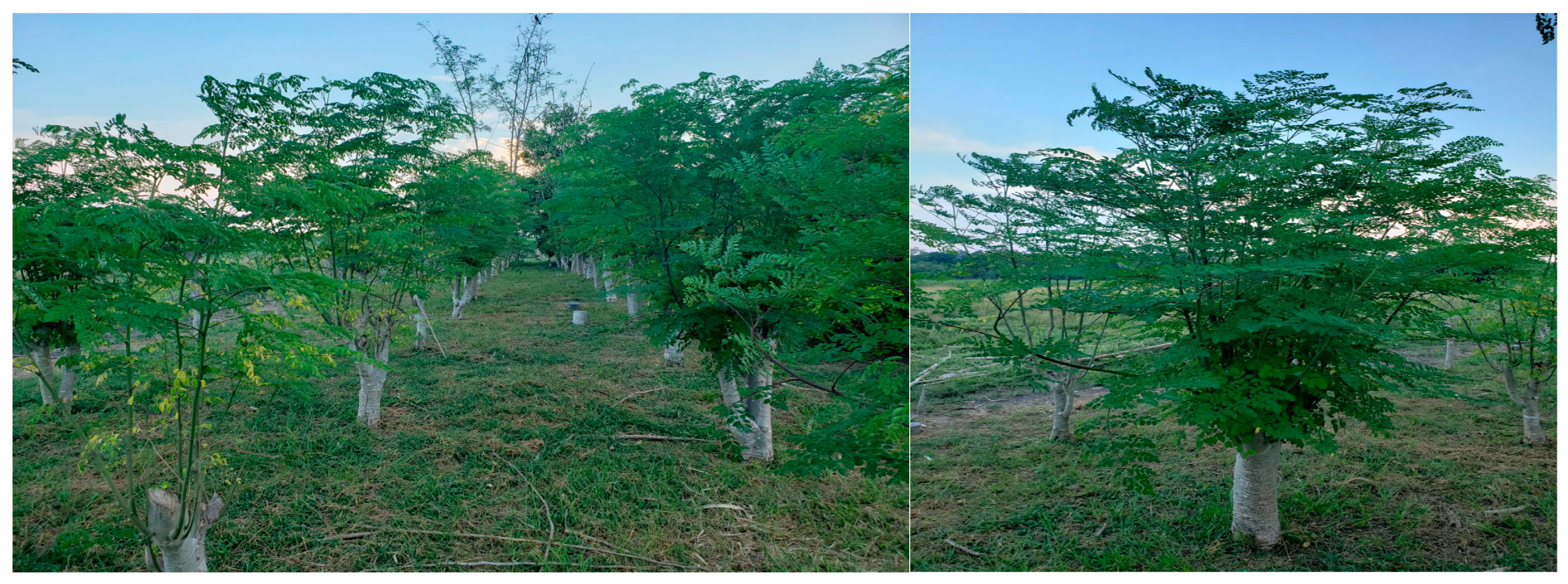
2.1. Study Site

BD Moringa^® is the commercial brand of the company “Ingeniería Agropecuaria del Papaloapan S.P.R de R.L.” located in Tierra Blanca, Veracruz, Mexico. It has a production system characterized by low technology. Currently, the company has a total of 1150 four-year-old moringa trees in production (Figure 1).

2.2. Stage 1: Analysis of the Current Situation of the Study Area

Characterization of the Process: The production system under study was mapped using process flow diagrams [91], value stream mapping (VSM) [92], plant layout design [93], and flowcharts [94].

Identification of Study Variables: The variables analyzed during the research were as follows: For VSM, the effective capacity, cycle time, and TAKT TIME (time required to complete one unit to meet demand) in the production process were analyzed. Descriptive statistics (mean and standard deviation in minutes) were obtained for each stage of the process. For the simulation model, the average global manufacturing time in minutes was calculated as the total finished product, with the batch size restriction of 12 kg of raw material powder. The daily production of 90-capsule bottles was also determined. Production costs were calculated monthly, including raw material procurement, processing costs, indirect costs, inputs, advertising, and administrative expenses. The economic analysis included the net present value, internal ratio of return, benefit–cost ratio, and payback period. The unit analysis involved calculating production costs per bottle, capsule processing per hour, labor costs, and the required personnel for the production process for the three simulation scenarios.

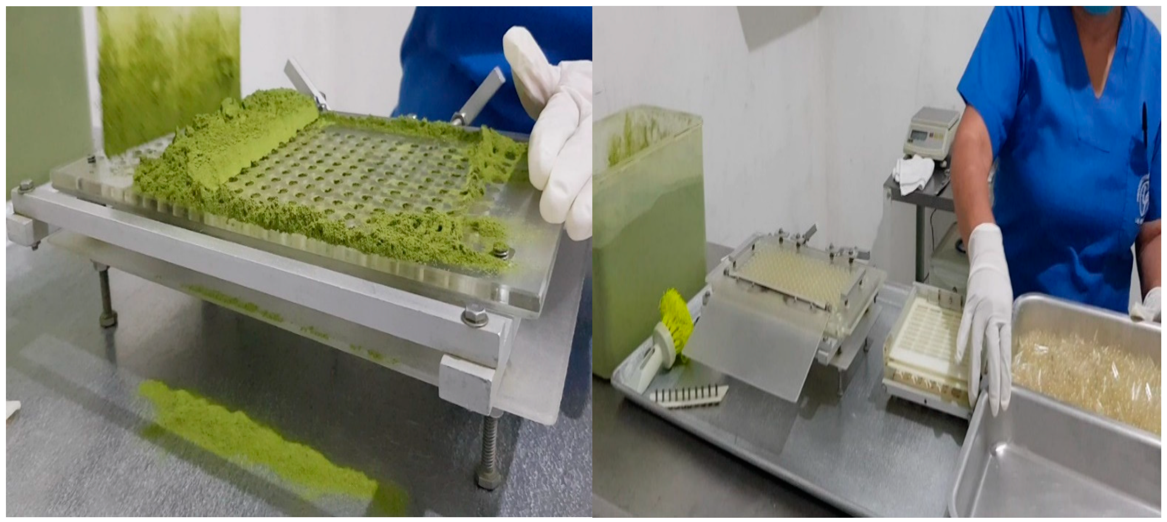
2.3. Stage 2: Analysis of the Key Process, Encapsulation

During the research stay, the process was characterized, and 10 activities were identified for the development of the final product. The focus was on analyzing the encapsulation process, as it was determined to be the key process affecting the production system, acting as a bottleneck. The process flow diagram was developed following the elements established [95].

Analysis of technology used in the process: The production process was identified, and each of its components was analyzed through interviews with staff and non-participant observation to understand the processes and equipment in detail [96].

Process simulation: For the development of the simulation, the methodology of [97] was used (Figure 2), using Arena Software (Simulation software version 16, Rockwell Automation, Milwaukee, WI, USA).

Data collection: For data sampling, a record of encapsulation process times was made at different times during a workday, recorded in minutes. To collect these time data, visits were made over a period of 90 days, during which 50 samples were taken according to the different activities required for the encapsulation production process (

Table 1. Methodological record for time recording.

Sampling Technique: Random Sampling Instrument: Time Recording Table
Type of instrument	Time Sheet	Target Population	Units produced in the production process
Study Representativeness	Local	Sample Frame	Number of daily lots, 24 h
Number of Sampling Points	10	Sampling Method Unit Selection	Systematic
Number of Data per Point	50	Data Collection Method	Digital Stopwatch
Total Number of Samples	50	Dates of Data Collection	Phase1 March (2022) Phase 2 April (2022)
Sampling Design, Measurement Instrument, Capture, and Analysis.	E.D.P., E.A.B.-T., R.Á.M.-A, J.M.C.D., M.J.H.-R., M.E.G.-R and O.B.-S.	Confidence Level%	95%
Field operation, supervision	E.D.P.	Margin of error %	5%

).

Data Sampling: The sampling frame consisted of sampling units equivalent to the minutes and seconds of a day of production. The unit of observation for quality characteristics corresponded to the time at each workstation, according to the production process flow diagram. It was decided, in conjunction with the factory personnel, to take the times using systematic sampling [99] at 10 sampling points on the production line, at 30-min intervals, forming a pilot sample of 50 records, which correspond to 20% of the shift time. We began with the first sampling point randomly during one shift using the following procedure:

• The sampling frame was divided into segments, where n is the desired sample size. The size of these segments will be K = N/n, where K is called the interval or elevation coefficient;
• Starting number: A random integer, r, less than or equal to the interval was obtained. This number corresponds to the first subject we will select for the sample within the first segment into which we have divided the population;
• Selection of the remaining n − 1 individuals: The individuals were selected starting from the randomly selected individuals, using an arithmetic sequence, selecting individuals from the remaining segments into which the sample was divided, occupying the same position as the initial subject. This is equivalent to selecting individuals with the following equation:

r, r + K, r + 2K, r + 3K, …, r + (n − 1)K

(1)

This method was chosen because it is commonly used in inspection and quality control due to its high speed and low variance [100]. The optimal sample size was determined to be 50 data points taken during a full day of work. Given the nature of the process, it was not feasible to select large samples during the process [101]. Additionally, the production line is continuous, meaning that once the process starts, products are generated continuously. Therefore, the sampling units are ordered sequentially, in line with the suggestion by [102] for choosing the sample size, as follows: “some amount of empirical judgement is required”. On the other hand, Refs. [103,104,105] suggest the application of monitoring, in which the expert selects a sample of process observations ordered over time as historical data for parameter estimation.

Field instrument: An Excel database was designed to capture the input data for the variables for each activity based on Shewart control charts [106]. The data were collected during March and April 2022, when a random sample of data was obtained for each activity of the production process.

Determination of the type of distribution to which the data fit: Romero-Saldaña [107], states that goodness-of-fit tests are used to verify that the data obtained from the sample fit a particular known probability distribution. For this purpose, the software Stat:Fit Student Version, 3.1.2.1 (Geer Mountain Software Corp, Pinehurst, NC, USA) was used to determine the type of distribution that the data fit and to determine the specific probability distribution that best fits each operation.

The Kolmogorov–Smirnov and Anderson–Darling tests were applied to determine which curve the data fit, and the mean and standard deviation were obtained for each stage of the process in order to obtain sufficient statistical evidence to assert that the data fit some probability distribution, which will be the basis for programming in each of the stages of the simulation model [108].

Model validation: Model validation is a mathematical procedure whose importance lies in ensuring that the data generated by the simulation are statistically similar to those of the real system, thus providing a model capable of emulating the real system and being an effective tool in decision-making. For validation, the paired t-test was used, with the following null hypothesis:

H₀: 

There is no significant difference between the data from the simulator and those from the real system.

H₁ :

There is a significant difference between the data from the simulator and those from the real system.

To achieve this, it is assumed that x₁, x₂ … x_k are observations from a real system, and y₁, y₂, … y_l are data produced by a simulation model. It is necessary to compare the data in data sets to determine if the model is a valid representation of the system.

The procedure used to perform this validation was as follows: m independent sets of data from the system and n sets of data from the model are collected. Let xj be the average of the observations in the J-th set of the system, and let yj be the average of the observations in the j-th set of data from the model. The xj’s are independent and identically distributed (IID) random variables with a mean of µx = E(xj), and the yj’s are IID random variables (assuming that the n sets of data were obtained from different replications) with a mean of µ_y = E(y_j). Therefore, the model was compared with the system by constructing a confidence interval for the following:

Z = µx − µy

(2)

Formulas for the paired t-test, as follows:

$$Z_i=X_I-Y_i$$

(3)

The observed difference between µ, as follows:

$${\displaystyle \frac{Z_{\left(n\right)}={{\displaystyle \sum }}_{i=1}^n{Z}_i}{n}}$$

(4)

$$\widehat{V}\mathrm{ar}\left[Z\left(n\right)\right]={\displaystyle \frac{{{\displaystyle \sum }}_{i=1}^n{\left[Z_{\mathrm{i}}-{\overline{Z}}_{\left(n\right)}\right]}^2}{n\left(n-1\right)}}\dots .$$

(5)

The confidence interval is 100 (1 − α), as follows:

$${\overline{\mathrm{Z}}}_{\left(n\right)}\pm {\mathrm{t}}_{n-1,1-\mathsf{\alpha }∕2}\sqrt{\hat{\mathrm{V}}\mathrm{ar}\left({\overline{\mathrm{Z}}}_{\left(n\right)}\right)}$$

(6)

Let l(α) and µ(α) be the lower and upper confidence limits, respectively. If ø$\varnothing \notin \left[l_{\left(\alpha \right)},{\mu }_{\left(\alpha \right)}\right]$, then the observed difference between µ_x and µ_y is as follows:

$${\overline{X}}_{\left(m\right)}-{\overline{Y}}_{\left(n\right)}$$

It is stated that it is statistically significant at level α. This is equivalent to rejecting the null hypothesis, as follows:

$$H_0:{\mu }_x={\mu }_y$$

In favor of the alternative, as follows:

$${\mathrm{H}}_1:{\mathsf{\mu }}_{\mathrm{x}}\ne {\mathsf{\mu }}_{\mathrm{y}}\mathrm{A}={\mathsf{\pi }\mathrm{r}}^2$$

If ø$\varnothing \notin \left[l_{\left(\alpha \right)},{\mu }_{\left(\alpha \right)}\right]$, any observed difference between µx and µy is not statistically significant at level α and can be explained by random fluctuations, thus accepting that the model is valid.

Number of replications: To ensure that the output data from the simulation are as accurate as possible and that the number of obtained data is sufficient, the initialization bias in the runs was considered [108]. Since a terminal-type simulation was used, the initialization bias was not considered regarding the number of runs (replicas). For models with highly varied output data, more than five replicas are needed to obtain satisfactory results. Therefore, to make decisions, once the simulation is validated, it is necessary to know the number of replications (independent simulations). For this purpose, the procedure for estimating the mean µ = E(x) with a specific error was used after the model had been validated. If the estimator $\overline{X}$ is such that $|\overline{\mathrm{x}}-\mathrm{\mu }|=\mathrm{\beta }$, then it is said that $\overline{X}$ has an absolute error $\beta$. If replications of the same simulation are made until half of the confidence interval, given the following:

$${\overline{X}}_n^{}\pm t_{n-1,1-\alpha /2}\sqrt{{\displaystyle \frac{s^2\left(n\right)}{n}}}$$

(7)

Is less than or equal to $\beta$ (where $\beta$ ˃ 0, and $\beta$ is the absolute error), then:

$$1-\alpha \approx p\left(\overline{X}-half\le \mu \le \overline{X}+half\right)$$

$$=p\left(\left|\overline{x}-\mu \right|\le half\right)$$

$$\le p\left(\overline{X}-\mu \le \beta \right)$$

Therefore, $\overline{X}$ has an absolute error of $\beta$ with a probability of approximately 1 − $\alpha$.

In other words, if 100 independent confidence intervals are constructed at 90%, it is expected that $\overline{X}$ has an absolute error of $\beta$ in 90 cases; around 10 intervals, the absolute error would be greater than $\beta .$ A confidence interval for $\mu$ based on a fixed number of replications n was constructed. Assuming that the estimator of the population variance does not change appreciably as the number of replications increases, an approximate expression for the total number of replications n*$\left(\beta \right)$ required to obtain an absolute error of $\beta$ is given as follows:

$$n*\left(\beta \right)\left\{i\ge n:t_{i-1,1-\alpha /2}\right.\sqrt{{\displaystyle \frac{s^2\left(n\right)}{i}}}\le \beta$$

It is possible to determine n*($\beta )$ by increasing i by one until a value of i is obtained, as follows:

$$\left\{t_{i-1,1-\alpha /2}\right.\sqrt{{\displaystyle \frac{s^2\left(n\right)}{i}}}\le \beta$$

(8)

2.4. Stage 3: Analyzed Simulation Scenarios

To make a decision that allows for improving the process situation, three scenarios were designed, as suggested by the company’s manager. The first scenario consisted of comparing the following:

• Maintaining the natural conditions of the model, one encapsulator producing 200 capsules with one operator;
• Increasing to an additional encapsulator with the same characteristics as the existing one, which will require two operators;
• An encapsulator with a capacity of 800 capsules, operated by one person.

This decision was made because it was determined that the key process was encapsulation.

Economic Evaluation: Economic and Financial Indicators

The economic variables for the financial evaluation of the production process of Moringa oleifera leaf powder capsules were calculated according to the methodology established by [109] for evaluating investment projects regarding the internal rate of return (IRR), the benefit–cost ratio (B/C), and the net present value (NPV).

3. Results and Discussion

The processing times and the feasibility analysis of the production of Moringa oleifera capsules require a comprehensive analysis that starts with process characterization. In the empirical evidence in the field of Moringa oleifera knowledge, economic data and production processes have not been reported; despite the wide range of studies about this tree with other types of study variables [110], these findings are pioneering in studying the variables of interest for implementing small capsule production factories. Within the existing knowledge, no previous studies were found in the field of simulation, engineering, and agronomy.

3.1. Process Characterization

To deeply understand the production process, the creation of the process flow diagram (Figure 3) and the value stream mapping (VSM) (Supplementary Materials: Figure S1; Value Stream Mapping (VSM) of the capsule production process of Moringa oleifera leaf) showed a vision of the information flow during the production process of Moringa oleifera encapsulation. With VSM, the activities that are functioning correctly were identified, as well as those activities that do not add value to the production process and can be corrected to improve the process.

3.2. Analysis of Study Variables in VSM

The previous VSM of the company indicated that, during an 8 h period, production starts with an inventory of 5000 g of raw material, allowing for the processing of 62 units of 200 capsules in a working day. Therefore, it is necessary to work 10 h, achieving 6.2 units per hour, and each finished unit is produced in 9.67 min.

To obtain the current situation of the company, it was necessary to complement the VSM with the following three important concepts: effective capacity, cycle time, and TAKT TIME (time required to complete one unit to meet the demand) [111]. It can be observed that the company’s effective capacity is 63%, meaning that it is capable of satisfactorily fulfilling 63 of 100 units. The process efficiency is 43%, which is relatively low. Therefore, it is common to require extra time on days of increased production and the hiring of temporary personnel to meet market demands. The current cycle time of the company to produce two units is 25,820 s. The TAKT time is 221.76 s, indicating that this is the time within which a customer can acquire a product or service from the company. In other words, the production rate should be adjusted as close as possible to the TAKT time. Overall, the VSM identified areas for improvement in raw material reception, raw material selection, sterilization, and the grinding–pulverizing process.

3.3. Analysis of the Key Process, Encapsulation

The encapsulation process is critical to the system. During this process, the pulverized raw material reaches a manual encapsulator, which is operated by one worker. This manual encapsulator interrupts the continuous flow of the process due to its limited capacity of 200 capsules. Therefore, this stage was identified as the bottleneck of the system (Figure 4). For this reason, the simulation scenarios focused on analyzing the replacement of this encapsulator model, considering the following criteria:

• Maintaining the natural conditions of the model using a 200-capsule encapsulator with one worker;
• Increasing to an additional encapsulator with the same characteristics as the existing one, requiring two workers;
• An encapsulator with a capacity of 800 capsules, with one operator.

3.4. Simulation Model Description

In the Supplementary Materials: Figure S2: Simulation model of the Moringa oleifera leaf powder encapsulation process, the simulation model is depicted, in which modules available in the simulator were used to create entities and assign them the corresponding attributes. Programming initiation began with a “create” module named “raw material supply” to track the arrival of raw materials every 14 days. The “create” window is a constant expression set to 14 days with a maximum of 120 created entities.

The second module is a batch named “6-kg” functioning as a grouping mechanism within the simulation model. Batches can be grouped permanently or temporarily; in this case, they are permanently grouped into 6 kg batches. The third module, named “raw material reception”, is performed using a process module, which is used to occupy and release a resource. In this case, 6 kg batches are received and passed on to the next module. The following modules are processes named basic cleaning, leaf selection, sterilization, crushing, grinding, and secondary sterilization.

The time for each process is added to the corresponding entity in each module. Once the assigned time is completed, it is released to the next module. For instance, in the leaf selection process module, an average time in minutes (58.7), a standard deviation (0.583), and a process type (standard) are determined.

After the process modules, a “route1” is observed in the model, which is used for direct translation from one station to another. An output station is not required for this module, as it automatically connects to the next station. The clock in the animation toolbar is an important addition and configuration, as it helps identify exact moments in which anomalies in the system might occur.

The next module is “station1”, which together with “route1”, is used to transfer from one station to another. Following this module, there is a component called separate, which is referred to as “approximately 100 g”. It is used to replicate incoming entities into multiple entities or to divide a previously grouped entity. It was used to group 100 g of raw material. In the next three modules, we have process modules, which are grouped to receive and release the resource. They receive the specified quantity within the programmed time and release it to the next module. After these three modules, there is a record module named “count”, which was used to keep track of how many orders are processed within a programmed time.

The following module is “decide1”, which is the last packet (pkt); this one is used to decide whether to proceed to the next module or return to the previous one in the model’s path. This module has two entity outputs, one true and one false. When analyzing the model and using the true output, it indicates that the packets are finished, and a product output is generated. In the case of a negative decision in the simulation, it records the completed packets and returns to the previous module until new packets arrive. This process continues until the programmed number of packets is completed.

The second “decide1” module was necessary to generate a report on the daily production, creating a multiple-output report. For example, if it is within the first 8 h of the process, it is considered the first day. If it is between 8 and 16 h, it is the second day, and if it is between 16 and 24 h, it corresponds to the third day, and so on. All these times are measured in minutes. The parameters of the simulation model are shown in Supplementary Materials: Figure S2: Simulation model of the Moringa oleifera leaf powder encapsulation process 120 batches (24,000 capsules).

3.5. Determination of the Type of Distribution to Which the Data Fit

In

Table 2. Data obtained from the goodness fit test of observed data from the production process.

Process Stage	Measures of Central Tendency (min)		Test Statistic						Data Distribution Fit	Theoretical Distribution Statistics.
			Kolmogorov–Smirnov			Anderson–Darling
	$\overline{\mathit{X}}$	s	Statistic KS	Alpha	p	Statistic AD	1-α	p		Minimum Value	µ	σ
Raw Material Reception	39.99	3.663	0.116	0.005	0.477	1.3	0.005	0.232	Log normal	30	2.25	0.395
Basic Cleaning	3.78	0.310	0.137	0.005	0.275	1.99	0.005	0.934	Log normal	3	−0.320	0.496
Leaf Selection	58.87	0.583	0.131	0.005	0.329	1.51	0.005	0.174	Uniform	58.02
Basic Sterilization	4.79	0.116	0.125	0.005	0.382	0.73	0.005	0.534	Log normal	4.49	−2.23	0.14
Crushing	39.02	2.66	0.158	0.005	0.145	2.18	0.005	0.073	Log normal	33.895	1.66	0.582
Pulverization	40.00	3.94	0.175	0.005	0.008	2.25	0.005	0.004	Log normal	30	2.23	0.51
Secondary Sterilization	120.12	0.142	0.102	0.005	0.635	0.427	0.005	0.821	Log normal	119.81	0.0097	0.129
Encapsulation	21.84	1.55	0.00973	0.005	0.694	0.418	0.005	0.831	Log normal	19.49	0.907	0.540
Business Labeling	4.51	0.570	0.168	0.005	0.106	1.44	0.005	0.192	Log normal	3.45	0.329	0.441

, the Kolmogorov–Smirnov and Anderson–Darling tests were applied to determine which curve the data fit, and the mean and standard deviation were obtained for each stage of the process in order to obtain sufficient statistical evidence to assert that the data fit some probability distribution, which will be the basis for programming in each of the stages of the simulation model [108].

3.6. Model Validation

For the validation, the paired t-test was applied to the model. This was performed to verify the results obtained from the simulation with real data using the time it takes to produce 120 batches, which is 24,000 capsules. The following working hypothesis was tested:

• X = The time in minutes it takes to produce 120 batches (24,000 capsules) in the real process.
• Y = The time in minutes it takes to produce 120 batches (24,000 capsules) in the created simulation model.

The results of the 2-week, 10-day runs are shown in

Table 3. Two-week simulation runs.

	Real	Simulated
Runs	Xj	Yj	Zj = Xj − Yj	${\left({\mathit{Z}}_{\mathit{J}}\mathbf{-}{\overline{\mathit{Z}}}_{\mathbf{15}}\right)}^{\mathbf{2}}$
1	3465.66	3469.00	−3.34	76.38
2	3490.00	3467.97	22.03	276.55
3	3485.22	3439.94	45.28	1590.41
4	3460.81	3448.79	12.02	43.82
5	3440.12	3434.99	5.13	0.07
6	3450.23	3450.19	0.04	28.72
7	3445.30	3476.31	−31.01	1325.68
8	3463.12	3470.78	−7.66	170.56
9	3459.15	3461.51	−2.36	60.21
10	3449.51	3448.08	1.43	15.76
11	3455.28	3456.14	−0.86	39.18
12	3482.27	3444.58	37.69	1042.64
13	3443.08	3444.25	−1.17	43.16
14	3462.00	3465.90	−3.9	86.49
15	3463.23	3455.42	7.81	5.8
		Total	81.13	4805.43
		Average	5.4

, for which a 95% confidence interval was considered for Z where ZJ = XJ − YJ. A 95% confidence interval was considered for Z where ZJ = XJ − YJ. Applying the formulas described in the previous section for the paired t-test, the results are shown in Table 3.

$$5.40$$

$$\widehat{V}ar\left[Z\left(n\right)\right]={\displaystyle \frac{{{\displaystyle \sum }}_{i=1}^{15}{\left[z_{\mathrm{i}}-{\overline{z}}_{\left(15\right)}\right]}^2}{15\left(15-1\right)}}={\displaystyle \frac{4805.43}{\left(15\right)\left(14\right)}}=22.88$$

$${\overline{Z}}_{\left(n\right)}\pm t_{n-1,1-\alpha ∕2}\sqrt{\widehat{V}ar\left({\overline{Z}}_{\left(n\right)}\right)}$$

$$-5.40\pm t_{14,0.975}\sqrt{22.88}$$

$$-5.40\pm 2.145\sqrt{22.88}$$

$$-5.40\pm 10.26$$

(−15.66, +4.86)

It is observed that the resulting interval includes zero; therefore, the null hypothesis cannot be rejected. Thus, it is concluded that with a 95% confidence level, the model is valid and representative of the real system. Any observed difference between µx and µy is statistically negligible and can be explained by random fluctuations.

3.7. Number of Replications

To make decisions once the simulation model has been validated, it is necessary to know the number of replications (independent simulations). For this purpose, the procedure for estimating the mean with a specific error was used, as shown in

Table 4. Replications carried out and their average manufacturing time.

Replications or Runs	Average Manufacturing Time (min)
1	3469
2	3467.97
3	3439.94
4	3448.79
5	3434.99
6	3450.19
7	3476.31
8	3470.78
9	3461.51
10	3448.08
11	3456.14
12	3444.58
13	3444.25
14	3465.9
15	3455.42
Average	3455.59
Standard Deviation	12.4949

.

For the calculation of the number of replications, a sample of 15 data points of the average time between each production process was used, with an absolute error of 5.4 s and a confidence level of 95%. Substituting the obtained values into the equation, the input data are as follows:

$$\overline{X}=3455.59,S=156,\beta =5.4,\alpha =0.1$$

$$\min \left\{i\ge 15:t_{0.95}\right.\sqrt{{\displaystyle \frac{156}{i}}}\le 5.4\}$$

For 15 replications, the equation is as follows: i = 15

1.660$\sqrt{{\displaystyle \frac{156}{15}} }=$ 5.3 ≤ 5.4 The condition is met.

Therefore, it is determined that the simulation model is statistically valid with an optimal number of replications of 15 runs.

3.8. Analyzed Simulation Scenarios

Table 5. Comparison of the 3 simulation scenarios for the encapsulation stage.

	Parameters of the Models
Simulation Scenario	Total Time			Encapsulation			Personnel Occupied	Worked Hours	Worked Days	Time Reduction (%)	Downtime (Hours)
	Minutes	Hours	Working Days	Capsules	Batches	Kg
1E200C	3455	57.5	7	24,000	120	12	1	56	7	35	0
2E200C	2263	37.7	4	24,000	120	12	2	32	4	24	24
1E800C	1415	23.5	2	24,000	120	12	1	16	2	60	35

compares the simulated times considering three simulation scenarios, which included the following: one encapsulator of 200 capsules (1E200C), two encapsulators of 200 capsules (2E200C), and one encapsulator of 800 capsules (1E800C). It is clearly observed that the 1E200C encapsulator requires the most time to complete the batch. In scenario 1E200C, the processing time in hours was 57.5 min, with 2E200C it was 37.7 min, and with 1E800C, it was 23.5 min. The production capacity was set at 24,000 capsules due to raw material limitations. As for the reduction in time, it is noteworthy that models 1E200 (35%), 2E200C (24%), and 1E800C (60%) show significant reductions. Furthermore, with the 1E800C model, only 2 working days (16 h) are required, while 4 working days (32 h) are needed with 2E200C, and 7 working days (56 h) are needed with 1E200C.

The results indicated that the working days of the different scenarios show a reduction in working days based on the model. Thus, it is evident that with the 1E800C model, only 23.5 h (2 days) are required, with 2E200C it is 37.7 (4 days), and with 1E200C it is 57.5 (7 days). This indicates that with this model, the labor cost is high because personnel are required throughout the week. However, with the 1E800C and 2E200C models, it is noticeable that personnel are only partially occupied. Therefore, raw materials would need to be increased, and idle times of 24 and 35 h per week, respectively, would need to be eliminated if these models are implemented.

On the other hand, in

Table 6. Cost comparison of the three scenarios of the simulation of the whole production process.

Simulation Scenario	Total Process Time			Limit of Simulation Model Due to Raw Material Limitation per Week			Larger Queue in System		Personnel	Labor Cost (USD)	Days Occupied per Week
	Minutes	Hours	Working Days	Capsules	Batches	Kg
1E200C	3455	57.5	7	24,000	120	12	Encapsulation	1	830.51	7	3.93
2E200C	2263	37.7	4	24,000	120	12	Encapsulation	2	474.58	4	3.64
1E800C	1415	23.5	2	24,000	120	12	Encapsulation	1	237.29	2	3.45

, the cost comparison of the three scenarios shows that with 1E800C, the production cost per bottle is 58.11. This is because fewer personnel hours are required to meet the quota of 24,000 capsules (266 units of 90 capsules) per week. Currently, with the 1E200C model, the production cost amounts to USD 3.93, as 7 working days per week are required to meet the quota. Finally, with 2E200C, the cost was USD 3.64, with 4 working days required to complete the quota. These results confirm that increasing production capacity reduces production costs, but the alternative of producing more raw materials must be sought to avoid downtime or hiring personnel only for the days worked and thus avoid losses.

Regarding the waiting lines (Table 6), it is confirmed that the encapsulation process is critical in the production process, as the average waiting times in the queue in the system for the 120 batches to be processed were 57.52 h for 1E200C, 37.7 h for 2E200C, and 23.5 h for 1E800C, indicating that with this last model, the average waiting time is reduced by 60%.

3.9. Moringa oleifera Capsule Production Costs and Financial Evaluation

Once the simulation of the base case has been carried out and the results of the main technical-economic indicators of the process in question have been obtained, as well as the technical characteristics of the equipment used, the selling price of bottles of 90 capsules of Moringa oleifera is set at an average of USD 10.68. The economic study was carried out by calculating the NPV, IRR, and B/C, among other indicators that are shown in the income statement (

Table 7. Comparison of production costs of Moringa oleifera leaf powder capsules and financial evaluation (USD).

Costs	Unit of Measure	Unit Cost	Quantity	Year 1
Raw Material Reception
Disinfection	Month	148.31	12.00	1779.66
II. Processing
Labor	Month	0.18	12,000.00	8542.37
III. Indirect Costs
Energy	Month	332.20	12.00	3986.44
Water	Month	24.32	12.00	291.86
Telephony	Month	71.19	12.00	854.24
IV. Supplies
Raw Material per month	Kgs	1.42	1200.00	20,501.68
Packaging Material	Batch	0.65	12,800.00	8276.61
Advertising
Digital Media	Month	711.86	1.00	711.86
Transportation and Hauling	Freight	0.059	12,000.00	711.86
Distributable	Kgs	USD 0.45	12,000.00	316.78
Total Costs				45,973.36
Production Cost per Bottle of 90 capsules				3.59
Gross Profit				227,382.41
Administrative Expenses				593.22
Fees	88.98	Month		1067.80
Stationery and Desk Supplies	29.66	Month		29.66
Depreciation and Amortization				3707.63
Total Costs and Expenses				50,274.21
Net Operating Income				22,3081.57
Final production cost per bottle of 90 capsules				3.93
Final production cost per capsule				0.043

).

The financial evaluation reflects the performance of the project and is of particular interest to the stakeholders of this proposal for making sound decisions. The evaluation will be based on the pro forma financial statements, which are projections of future expenses and revenues based on the company’s experience and future plans. The financial analysis aims to study the return and profitability on the investment of the project; among the aspects to be evaluated will be the net present value (NPV), internal rate of return (IRR), and benefit–cost ratio (B/C).

Table 8. Financial indicators of the production process for the model.

Financial Indicators
B/C Ratio	USD 5.03
NPV	USD 922,370.11
IRR	42.09%

shows the results of the main process indicators.

Benefit–Cost Ratio (B/C): This indicator measures the relationship between the project’s revenues and the costs incurred over its useful life, including the total investments. It takes the net present revenues and expenses from the income statement to determine the benefits for every peso invested in the project [112]. The possible results of the benefit–cost ratio are described as follows: (a) If the B/C ratio is greater than one, the project is acceptable because the benefits outweigh the costs 5.03. (b) If the B/C ratio is less than one, the model should be rejected because there is no benefit. (c) If the B/C ratio is equal to one, it is indifferent to carry out the project because there is no profit or loss. The business idea shows that for every USD 1 invested, it generates an additional USD 5.03.

The positive net present value (NPV) reflects that the project is profitable (it is financially feasible). Therefore, the decision that must be made is to execute the initiative. A positive NPV means that the project can generate enough money to recover the investment and make a profit [113].

On the other hand, the internal rate of return (IRR) represents the annual percentage rate that reduces the net present value of the project to zero. It shows investors the maximum interest rate at which they should take out loans without incurring future financial failures [114]. To achieve this, a rate applied to the net cash flow that generates an NPV equal to zero is sought. The model shows an average annual internal rate of return (IRR) of 42.09%. This indicates that despite the limitations, the company is viable since it meets the minimum profitability expectations. This is mainly due to the low production costs.

4. Conclusions

This work reaffirms the importance of applying modeling with Arena software in small businesses and linking with the productive sector of research institutions. The evidence presented determined that the waiting times in the queues of the simulation model showed the highest times in the encapsulation stage, identifying a bottleneck in this process. A simulation model was developed with Arena, which was validated by the plant manager. The model was designed and statistically validated, obtaining information that allowed for decision-making evidence. It was found that the company has a raw material limitation that allows it to produce 12,800 units of 90 capsules per year. It is recommended to establish the 1E800C encapsulator, as it reduces processing times by 60%. Additionally, it will reduce the overall production costs by 12.23%, which represents USD 0.48 per unit produced. Economically, this will allow for an additional profit of USD 6150.50.

With the financial engineering calculations, the profitability of this new type of agribusiness in Mexico was confirmed. However, work should be conducted on the development of a business plan that allows for the commercialization of the product through various distribution channels to guarantee the proper sale of the product and with a higher volume. Furthermore, with the data presented, the hypothesis proposed is accepted, which states that process simulation with Arena in a small agricultural business producing Moringa oleifera capsules is suitable for estimating processing times, and its production is technically and economically viable.

In this case study, despite the deficiencies in the production process of Moringa oleifera capsules, it is economically profitable. Therefore, it is recommended that other producers undertake the production of Moringa oleifera capsules due to its profitability, which is above banking reference rates and inflation, in addition to the low operating costs, as indicated by the cost–benefit ratio.

Future Lines of Research

During the development of this work, the following lines of research are proposed in the field of Moringa oleifera knowledge, in which information is limited: (1) Evaluate drying systems for Moringa oleifera leaves to ensure the permanence of nutrients and incorporate a quality and traceability control in the system that involves both the field and the factory. (2) Determine the optimal size of plots planted with Moringa oleifera trees to design optimal plant sizes. (3) Determine the production capacity of green Moringa oleifera leaf material, and define the number of kilograms that can be produced under different soil conditions under rainfed and irrigation conditions for processing. Finally, in the primary sector, simulation can be used to model and optimize quality control processes, including raw material inspection, process monitoring, and the evaluation of the quality of the final product to ensure compliance with quality and food safety standards. In addition, in production scheduling and management, simulation can optimize the resource allocation and production costs of other products based on Moringa oleifera and mitigate risks associated with the production of food supplements, including cross-contamination, process variability, and regulatory compliance.

References

1. Rockwell Automation Inc. Arena® Simulation Software, version 16; Rockwell Automation Inc.: Milwaukee, WI, USA, 2017. Available online: https://www.rockwellautomation.com/es-mx/products/software/arena-simulation/case-studies/hospital-simulation-prevents-unnecessary-investment.html (accessed on 17 May 2024).
2. Roungas, B.; Bekius, F.; Verbraeck, A.; Meijer, S. Improving the decision-making qualities of gaming simulations. J. Simul. 2021, 15, 1–14. [Google Scholar] [CrossRef]
3. Black, L.; Tarquin, A. Economic Engineering, 7th ed.; Mc Graw Hill: Mexico City, Mexico, 2012. [Google Scholar]
4. Troncoso-Palacio, A.; Neira-Rodado, D.; Ortíz-Barrios, M.; Jiménez-Delgado, G.; Hernández-Palma, H. Using Discrete-Event-Simulation for Improving Operational Efficiency in Laboratories: A Case Study in Pharmaceutical Industry. In En Lecture Notes in Computer Science; Springer International Publishing: Cham, Switzerland, 2018; pp. 440–451. [Google Scholar] [CrossRef]
5. Reyes Mejia, R.; Troncoso Mendoza, B.; Troncoso Palacio, A. Discrete Event Simulation Applying Lean methodologies: Case study. Wooden Sector. Int. J. Manag. Sci. Oper. Res. 2020, 4, 440–451. [Google Scholar] [CrossRef]
6. Robinson, S. Simulation: The Practice of Model Development and Use; Red Globe Press: New York, NY, USA, 2020. [Google Scholar]
7. Frough, O.; Khetwal, A.; Rostami, J. Predicting TBM utilization factor using discrete event simulation models. Tunn. Undergr. Space Technol. 2019, 87, 91–99. [Google Scholar] [CrossRef]
8. Tavasszy, L.A. Predicting the effects of logistics innovations on freight systems: Directions for research. Transp. Policy 2020, 86, A1–A6. [Google Scholar] [CrossRef]
9. Mendoza-Salguero, E.; De-La-Asunción-González, A.; Mejía-Vega, I.; Triana-Infante, J.; Troncoso Palacio, A. Análisis de Restricciones a Través Del Software Arena. Caso Empresa de Fabricación de Calzado. Boletín Innovación Logística Oper. 2022, 4, 8–15. [Google Scholar] [CrossRef]
10. Cuzcano Espino, L.A.; Vasquez Mamani, A.S.; Ramos Bonifaz, J.V.; Bazan-Aguilar, A. Design of SMARTER multi-criteria model to improve the productivity of the Order-picking process: Computational simulation. In En 21st LACCEI International Multi-Conference for Engineering, Education and Technology (LACCEI 2023): “Leadership in Education and Innovation in Engineering in the Framework of Global Transformations: Integration and Alliances for Integral Development”; Latin American and Caribbean Consortium of Engineering Institutions: Boca Raton, FL, USA, 2023. [Google Scholar] [CrossRef]
11. Rosova, A.; Behun, M.; Khouri, S.; Cehlar, M.; Ferencz, V.; Sofranko, M. Case study: The simulation modeling to improve the efficiency and performance of production process. Wirel. Netw. 2020, 28, 863–872. [Google Scholar] [CrossRef]
12. Johnstone, M.; Creighton, D.; Nahavandi, S. Simulation-based baggage handling system merge analysis. Simul. Model. Pract. Theory 2015, 53, 45–59. [Google Scholar] [CrossRef]
13. Huang, P.B.; Yu, T.-Y.; Chou, Y.-J.; Lin, Y.-C. Simulation method for dispatching national border security manpower to mitigate manpower shortage. J. Air Transp. Manag. 2016, 57, 43–51. [Google Scholar] [CrossRef]
14. Wong, T.C.; Xu, M.; Chin, K.S. A two-stage heuristic approach for nurse scheduling problem: A case study in an emergency department. Comput. Oper. Res. 2014, 51, 99–110. [Google Scholar] [CrossRef]
15. Valls, V.; Pérez, Á.; Quintanilla, S. Skilled workforce scheduling in Service Centres. Eur. J. Oper. Res. 2009, 193, 791–804. [Google Scholar] [CrossRef]
16. Çelik, G.; Sabuncuoğlu, İ. Simulation modelling and analysis of a border security system. Eur. J. Oper. Res. 2007, 180, 1394–1410. [Google Scholar] [CrossRef]
17. Bolkovska, A.; Petuhova, J. Simulation-based Public Transport Multi-modal Hub Analysis and Planning. Procedia Comput. Sci. 2017, 104, 530–538. [Google Scholar] [CrossRef]
18. Coronado-Hernández, J.R.; Ibáñez SF, U.; Gatica, G.; Rodríguez, M.A. Simulation Model of the Effect of the COVID-19 Biosecurity Protocol in the Queues for the Return to Face-to-Face Classes. Procedia Comput. Sci. 2023, 220, 904–908. [Google Scholar] [CrossRef] [PubMed]
19. Navarro, M. Simulation of a manual order picking system in a convenience store chain distribution center. In Proceedings of the 18th LACCEI International Multi-Conference for Engineering, Education, and Technology, Bogota, DC, Colombia, 27–31 July 2020; Available online: http://ndltd.ncl.edu.tw/handle/47300620219584190941 (accessed on 16 May 2024).
20. Ibrahim, M.F.; Putri, M.M.; Sari, D.N.; Utama, D.M. Industrial area weighbridge simulation model considering vehicle capacity and destination using arena software. In Proceedings of the 1st International Conference on Technology, Informatics, and Engineering, Malang, Indonesia, 28–29 July 2021; AIP Publishing: Melville, NY, USA, 2022. [Google Scholar] [CrossRef]
21. Pierreval, H.; Bruniaux, R.; Caux, C. A continuous simulation approach for supply chains in the automotive industry. Simul. Model. Pract. Theory 2007, 15, 185–198. [Google Scholar] [CrossRef]
22. Vidalakis, C.; Tookey, J.E.; Sommerville, J. Logistics simulation modelling across construction supply chains. Constr. Innov. 2011, 11, 212–228. [Google Scholar] [CrossRef]
23. Jaoua, A.; Riopel, D.; Gamache, M. A simulation framework for real-time fleet management in internal transport systems. Simul. Model. Pract. Theory 2012, 21, 78–90. [Google Scholar] [CrossRef]
24. Motraghi, A.; Marinov, M.V. Analysis of urban freight by rail using event based simulation. Simul. Model. Pract. Theory 2012, 25, 73–89. [Google Scholar] [CrossRef]
25. Köhler, J.; Brauer, C. Transformation in freight transport: New analysis requirements and potential modelling approaches. Transp. Res. Procedia 2023, 72, 4420–4427. [Google Scholar] [CrossRef]
26. Wu, W.; Shen, L.; Ji, X.; Jin, W. Analysis of freeway service patrol with discrete event-based simulation. Simul. Model. Pract. Theory 2014, 47, 141–151. [Google Scholar] [CrossRef]
27. Kamrani, M.; Hashemi Esmaeil Abadi, S.M.; Rahimpour Golroudbary, S. Traffic simulation of two adjacent unsignalized T-junctions during rush hours using Arena software. Simul. Model. Pract. Theory 2014, 49, 167–179. [Google Scholar] [CrossRef]
28. Fumasoli, T.; Bruckmann, D.; Weidmann, U. Operation of freight railways in densely used mixed traffic networks—An impact model to quantify changes in freight train characteristics. Res. Transp. Econ. 2015, 54, 15–19. [Google Scholar] [CrossRef]
29. Arathi, H.S.; Smith, T.J. Drought and temperature stresses impact pollen production and autonomous selfing in a California wildflower, Collinsia heterophylla. Ecol. Evol. 2023, 13, e10324. [Google Scholar] [CrossRef]
30. Saval, R.A. Remolque Autopropulsado Para Transporte De Embarcaciones; Maestria, Escola Tècnica Superior d’Enginyeria Industrial de Barcelona: Barcelona, Spain, 2020. [Google Scholar]
31. Mora, G.L.A. Transportation Logistics and Cargo Distribution, 23rd ed.; Ecoe Ediciones: Bogota, Colombia, 2023. [Google Scholar]
32. Sun, L.; Tirachini, A.; Axhausen, K.W.; Erath, A.; Lee, D.-H. Models of bus boarding and alighting dynamics. Transp. Res. 2014, 69, 447–460. [Google Scholar] [CrossRef]
33. Leich, G.; Bischoff, J. Should autonomous shared taxis replace buses? A simulation study. Transp. Res. Procedia 2019, 41, 450–460. [Google Scholar] [CrossRef]
34. Mepparambath, R.M.; Soh, Y.S.; Jayaraman, V.; Tan, H.E.; Ramli, M.A. A novel modelling approach of integrated taxi and transit mode and route choice using city-scale emerging mobility data. Transp. Res. 2023, 170, 103615. [Google Scholar] [CrossRef]
35. Delcea, C.; Chirita, N. Exploring the Applications of Agent-Based Modeling in Transportation. Appl. Sci. 2023, 13, 9815. [Google Scholar] [CrossRef]
36. Bae, J.W.; Lee, C.-H.; Lee, J.-W.; Choi, S.H. A data-driven agent-based simulation of the public bicycle-sharing system in Sejong city. Simul. Model. Pract. Theory 2024, 130, 102861. [Google Scholar] [CrossRef]
37. Gittins, P.; McElwee, G.; Tipi, N. Discrete event simulation in livestock management. J. Rural Stud. 2020, 78, 387–398. [Google Scholar] [CrossRef]
38. Rockwell Automation Inc. Arena® Simulation Software, version 16; Rockwell Automation Inc.: Milwaukee, WI, USA, 2017. Available online: https://www.rockwellautomation.com/es-mx/products/software/arena-simulation/case-studies/cancer-treatment-facility-reduces-patient-clinic-time.html (accessed on 17 May 2024).
39. Lee, K.-S.; Kim, S.-H.; Choi, W.-H. Self-Bag-Drop Simulation Development of Systems for Airport Baggage Handling System. Int. J. Adv. Sci. Technol. 2018, 118, 1–12. [Google Scholar] [CrossRef]
40. Cabrera, V.E.; Hildebrand, P.E.; Jones, J.W.; Letson, D.; de Vries, A. An integrated North Florida dairy farm model to reduce environmental impacts under seasonal climate variability. Agric. Ecosyst. Environ. 2006, 113, 82–97. [Google Scholar] [CrossRef]
41. Del Prado, A.; Misselbrook, T.; Chadwick, D.; Hopkins, A.; Dewhurst, R.J.; Davison, P.; Butler, A.; Schröder, J.; Scholefield, D. SIMSDAIRY: A modelling framework to identify sustainable dairy farms in the UK. Framework description and test for organic systems and N fertiliser optimisation. Sci. Total Environ. 2011, 409, 3993–4009. [Google Scholar] [CrossRef]
42. Jones, J.W.; Antle, J.M.; Basso, B.; Boote, K.J.; Conant, R.T.; Foster, I.; Godfray, H.C.J.; Herrero, M.; Howitt, R.E.; Janssen, S.; et al. Brief history of agricultural systems modeling. Agric. Syst. 2017, 155, 240–254. [Google Scholar] [CrossRef] [PubMed]
43. Herrero, M.; Havlik, P.; Valin, H.; Notenbaert, A.; Rufino, M.C.; Thornton, P.K.; Blummel, M.; Weiss, F.; Grace, D.; Obersteiner, M. Biomass use, production, feed efficiencies, and greenhouse gas emissions from global livestock systems. Proc. National Acad. Sci. USA 2013, 110, 20888–20893. [Google Scholar] [CrossRef] [PubMed]
44. Herrero, M.; González-Estrada, E.; Thornton, P.K.; Quirós, C.; Waithaka, M.M.; Ruiz, R.; Hoogenboom, G. IMPACT: Generic household-level databases and diagnostics tools for integrated crop-livestock systems analysis. Agric. Syst. 1996, 92, 240–265. [Google Scholar] [CrossRef]
45. Rufino, M.C.; Herrero, M.; Van Wijk, M.T.; Hemerik, L.; De Ridder, N.; Giller, K.E. Lifetime productivity of dairy cows in smallholder farming systems of the Central highlands of Kenya. Animal 2009, 3, 1044–1056. [Google Scholar] [CrossRef] [PubMed]
46. Ruiz, R.; Tedeschi, L.O.; Marini, J.C.; Fox, D.G.; Pell, A.N.; Jarvis, G.; Russell, J.B. The Effect of a Ruminal Nitrogen (N) Deficiency in Dairy Cows: Evaluation of the Cornell Net Carbohydrate and Protein System Ruminal N Deficiency Adjustment. J. Dairy Sci. 2002, 85, 2986–2999. [Google Scholar] [CrossRef]
47. Moore, A.D.; Donnelly, J.R.; Freer, M. GRAZPLAN: Decision support systems for Australian grazing enterprises. III. Pasture growth and soil moisture submodels, and the GrassGro DSS. Agric. Syst. 1997, 55, 535–582. [Google Scholar] [CrossRef]
48. Gerber, P.; Uwizeye, A.; Schulte, R.; Opio, C.; de Boer, I. Nutrient use efficiency: A valuable approach to benchmark the sustainability of nutrient use in global livestock production? Curr. Opin. Environ. Sustain. 2014, 9–10, 122–130. [Google Scholar] [CrossRef]
49. Van Wijk, M.T.; Rufino, M.C.; Enahoro, D.; Parsons, D.; Silvestri, S.; Valdivia, R.O.; Herrero, M. Farm household models to analyse food security in a changing climate: A review. Glob. Food Secur. 2007, 3, 77–84. [Google Scholar] [CrossRef]
50. Vayssières, J.; Guerrin, F.; Paillat, J.-M.; Lecomte, P. GAMEDE: A global activity model for evaluating the sustainability of dairy enterprises Part I—Whole-farm dynamic model. Agric. Syst. 2009, 101, 128–138. [Google Scholar] [CrossRef]
51. Lisson, S.; MacLeod, N.; McDonald, C.; Corfield, J.; Pengelly, B.; Wirajaswadi, L.; Rahman, R.; Bahar, S.; Padjung, R.; Razak, N.; et al. A participatory, farming systems approach to improving Bali cattle production in the smallholder crop–livestock systems of Eastern Indonesia. Agric. Syst. 2010, 103, 486–497. [Google Scholar] [CrossRef]
52. Rodriguez, D.; Cox, H.; deVoil, P.; Power, B. A participatory whole farm modelling approach to understand impacts and increase preparedness to climate change in Australia. Agric. Syst. 2014, 126, 50–61. [Google Scholar] [CrossRef]
53. Van Wijk, M.T.; Tittonell, P.; Rufino, M.C.; Herrero, M.; Pacini, C.; Ridder, N.D.; Giller, K.E. Identifying key entry-points for strategic management of smallholder farming systems in sub-Saharan Africa using the dynamic farm-scale simulation model Nuances-farmsim. Agric. Syst. 2009, 102, 89–101. [Google Scholar] [CrossRef]
54. Tensi, A.F.; Ang, F.; van der Fels-Klerx, H.J. Microbial Applications and Agricultural Sustainability: A Simulation Analysis of Dutch Potato Farms. SSRN Electron. J. 2023, 214, 103797. [Google Scholar] [CrossRef]
55. Goo, J.; Kwak, Y.; Kim, J.; Kang, J.; Shin, H.; Jo, S.-K.; Huh, J.-H. Development of early design tool for aquaculture buildings using building performance simulation: A case study of an indoor fish farm. Dev. Built Environ. 2024, 17, 100363. [Google Scholar] [CrossRef]
56. Konapathri, R.; Azimov, U. Assessment of ammonia distribution in a livestock farm using CFD simulations. Smart Agric. Technol. 2024, 7, 100376. [Google Scholar] [CrossRef]
57. Kongnuan, S.; Thongjub, N. A 3D-numerical simulation of groundwater flow and salinity in a rice field adjacent to a marine shrimp farm. Environ. Adv. 2024, 15, 100473. [Google Scholar] [CrossRef]
58. Kelton, W.D.; Zupick, N.; Ivey, N. Simulation with Arena (McGraw-Hill Series in Industrial Engineering and Management); McGraw-Hill Higher Education: New York, NY, USA, 2024. [Google Scholar]
59. Bawankule, G.; Urwate, P.; Chavan, K.; Inamdar, F.; Deshpande, S. Smart Precision Agriculture using IoT Simulation. Int. J. Adv. Res. Sci. Commun. Technol. 2024, 302–312. [Google Scholar] [CrossRef]
60. Fibigr, J.; Šatínský, D.; Solich, P. Current trends in the analysis and quality control of food supplements based on plant extracts. Anal. Chim. Acta 2018, 1036, 1–15. [Google Scholar] [CrossRef] [PubMed]
61. Valdés-Rodríguez, O. Socioeconomic characteristics and agricultural practices of Moringa oleifera Lam. Producers in México. Agro Product. 2019, 12, 2–8. [Google Scholar] [CrossRef]
62. Delfin-Portela, E.; Carrión-Delgado, J.M.; Garcia-Santamaria, L.E. Characterization of Moringa oleifera production systems in the state Veracruz. In Proceedings of the IV National Forum for the Evaluation of the Female Gender, Xalapa, Mexico, 23–24 October 2019; pp. 1–12. [Google Scholar]
63. Mathur, B. Trees for Life. En Conference, 4 de May of 2012; ACM Press: Sydney, Australia, 2005. [Google Scholar]
64. Gopalakrishnan, L.; Doriya, K.; Kumar, D.S. Moringa oleifera: A review on nutritive importance and its medicinal application. Food Sci. Hum. Wellness 2016, 5, 49–56. [Google Scholar] [CrossRef]
65. Dhakad, A.K.; Ikram, M.; Sharma, S.; Khan, S.; Pandey, V.V.; Singh, A. Biological, nutritional, and therapeutic significance of Moringa oleifera Lam. Phytother. Res. 2019, 33, 2870–2903. [Google Scholar] [CrossRef] [PubMed]
66. Thapa, K.; Poudel, M.; Adhikari, P. Moringa oleifera: A Review Article on Nutritional Properties and its Prospect in the Context of Nepal. Acta Sci. Agric. 2019, 3, 47–54. [Google Scholar] [CrossRef]
67. Dhiman, J. A Review on Medicinal uses of Moringa oleifera. J. Drug Deliv. Ther. 2023, 13, 197–201. [Google Scholar] [CrossRef]
68. Carrión, J.M.; Valdés Rodríguez, O.A.; Gallardo López, F.; Palacios Wassenaar, O.M. Agroecological potential of Moringa oleifera Lam. for the State of Veracruz. Rev. Mex. Sci. 2022, 13, 42–63. [Google Scholar] [CrossRef]
69. Fahey, J.; Fahey, J.W. Moringa oleifera: A review of the medical evidence for its nutritional, therapeutic, and prophylactic properties. Part 1. Trees Life J. 2005, 1, 1–15. [Google Scholar]
70. Babu, R.; Chaudhuri, M. Home water treatment by direct filtration with natural coagulant. J. Water Health 2005, 3, 27–30. [Google Scholar] [CrossRef] [PubMed]
71. Khawaja, T.M.; Tahira, M.; UI, I. Moringa oleifera: A natural gift—A review. J. Pharm. Sci. Res. 2010, 51, 6558–6563. [Google Scholar]
72. Bazán, C.J.C.; Reyes, S.V.A. Effects of Moringa of Hypertensive Adults. Bachelor’s Thesis, Cent Health San pedro, San pedro, CA, USA, 2018. [Google Scholar]
73. Famakinwa, A.; Oguntibejo, O.; Jideani, V. Fortification of Foodstuffs (Food Material) with Moringa oleifera; B P International: Meguro City, Japan, 2024; pp. 1–64. [Google Scholar] [CrossRef]
74. Su, X.; Lu, G.; Ye, L.; Shi, R.; Zhu, M.; Yu, X.; Li, Z.; Jia, X.; Feng, L. Moringa oleifera Lam.: A comprehensive review on active components, health benefits and application. RSC Adv. 2023, 13, 24353–24384. [Google Scholar] [CrossRef] [PubMed]
75. Diario Oficial de la Federación. Servicio de Información Agroalimentaria y Pesquera—SIAP, El poder de la Moringa en la Salud, s. f. (Mexico). 1 March 2023. Available online: https://www.gob.mx/siap/articulos/el-poder-de-la-moringa-en-la-salud?idiom=es#:~:text=Some%20benefits%20of%20the%20consumption%20of%20of%20of%20of,Control%20levels%20of%20cholesterol (accessed on 17 May 2024).
76. Bocarando-Guzmán, M.D.; Ríos-Corripio, M.A.; Hernández-Cázares, A.S.; Gómez-Merino, F.C.; Servín-Juárez, R. Caracterización de da Oferta de Moringa (Moringa oleifera Lam.) en México. Agro Product. 2020, 13, 2–8. [Google Scholar] [CrossRef]
77. Delfín-Portela, E.; Sanchez Galvan, F.; Bautista Santos, H.; Betanzo Torres, E.A. Scenario modeling of a Moringa capsule production process (Moringa oleifera Lam.) with Arena simulation software. In Proceedings of the International Congress on Sustainable Development and Renewable Energies (CIDSER), online, 21–22 September 2020; pp. 1–15. [Google Scholar]
78. Carrión Delgado, J.M.; Valdés-Rodríguez, O.A.; Palacios-Wasenaar, O.M.; Gallardo-López, F. Variations of the agroecological potential of Moringa oleifera Lam., in the presence of climate change scenarios in Veracruz, Mexico. Agro Product. 2023; early access. [Google Scholar] [CrossRef]
79. Olson, M.E.; Alvarado-Cárdenas, L.O. Where to grow the miracle tree, Moringa oleifera, in Mexico? An analysis of its potential distribution. Rev. Mex. Biodivers. 2016, 87, 1089–1102. [Google Scholar] [CrossRef]
80. Baek, C.-W.; Lee, J.-H. Quality evaluation of macaroons added with moringa leaf (Moringa oleifera Lam.) and green tea powder. Korean J. Food Preserv. 2020, 27, 555–565. [Google Scholar] [CrossRef]
81. Jikah, A.N.; Edo, G.I. Moringa oleifera: A valuable insight into recent advances in medicinal uses and pharmacological activities. J. Sci. Food Agric. 2023, 103, 7343–7361. [Google Scholar] [CrossRef] [PubMed]
82. Srivastava, S.; Pandey, V.K.; Dash, K.K.; Dayal, D.; Wal, P.; Debnath, B.; Singh, R.; Dar, A.H. Dynamic bioactive properties of nutritional superfood Moringa oleifera: A comprehensive review. J. Agric. Food Res. 2023, 14, 100860. [Google Scholar] [CrossRef]
83. Makkar, H.P.S.; Becker, K. Nutrional value and antinutritional components of whole and ethanol extracted Moringa oleifera leaves. Anim. Feed Sci. Technol. 1996, 63, 211–228. [Google Scholar] [CrossRef]
84. Castro, M. The moringa tree (Moringa oleifera Lam.): A renewable alternative for the development of the economic and environmental sectors of Colombia. Repos. Unimilitar Colomb 2013, 18, 3. [Google Scholar]
85. Gharsallah, K.; Rezig, L.; Rajoka, M.; Mehwish, H.; Chew, S. Moringa oleifera: Processing, phytochemical composition and industrial application. S. Afr. J. Bot. Afr. 2023, 160, 180–193. [Google Scholar] [CrossRef]
86. FAO. Abridged Version of The State of Food and Agriculture 2023; FAO: Rome, Italy, 2023. [Google Scholar] [CrossRef]
87. López-Martínez, L.X.; Dominguez-Ávila, J.A.; Salazar-Lopez, N.J.; Gonzalez-Aguilar, G.A. Quality Control and Safety of Moringa. En Biological and Pharmacological Properties of the Genus Moringa; CRC Press: New York, NY, USA, 2021; pp. 83–98. [Google Scholar] [CrossRef]
88. World Health Organization (WHO). WHO Global Database on Child Growth and Malnutrition; World Health Organization: Geneva, Switzerland, 2021. [Google Scholar]
89. Lafont Mendoza, J.; Negrete Humanez, W.; Espitia Arrieta, A. Estudios químicos realizados a la semilla de Moringa oleifera lam y su impacto en la salud humana: Una revisión teórica. In Science and Technology for Environmental, Cultural and Socioeconomic Development; Artemis Publishing House: Nashville, TN, USA, 2021; pp. 159–170. [Google Scholar] [CrossRef]
90. Calendario Martínez, B.; Ruiz Rosado, O.; Perez, P.; Martinez, A.; Vargas, L. Aplicación de modelos de simulación en el estudio y planificación de la agricultura, una revisión. Trop. Subtrop. Agroecosystems 2011, 14, 999–1010. [Google Scholar]
91. Theisen, M.F.; Flores, K.N.; Balhorn, L.S.; Schweidtmann, A.M. Digitization of chemical process flow diagrams using deep convolutional neural networks. Digit. Chem. Eng. 2022, 6, 100072. [Google Scholar] [CrossRef]
92. Horsthofer-Rauch, J.; Schumann, M.; Milde, M.; Vernim, S.; Reinhart, G. Digitalized value stream mapping: Review and outlook. Procedia CIRP 2022, 112, 244–249. [Google Scholar] [CrossRef]
93. Hawarneh, A.A.; Bendak, S.; Ghanim, F. Construction site layout planning problem: Past, present and future. Expert Syst. Appl. 2020, 168, 114247. [Google Scholar] [CrossRef]
94. Baca-Urbina, G. Project Evaluation, 7th ed.; McGraw-Hill Interamericana: Mexico City, Mexico, 2016. [Google Scholar]
95. Slack, N.; Jones, A. Operations & Process Management: Principles & Practice for Strategic Impact; Pearson Education: London, UK, 2021. [Google Scholar]
96. Hernández-Sampieri, R.; Fernández-Collado, C.; Baptista, L.P. Analysis of quantitative data. In Research Methodology; Mc Graw Hill: Mexico City, Mexico, 2020. [Google Scholar]
97. Law, A.M. Simulation Modeling and Analysis, 15th ed.; McGraw-Hill: New York, NY, USA, 2014. [Google Scholar]
98. Law, A.M. Simulation Modeling and Analysis Student Edition, 15th ed.; McGraw-Hill: New York, NY, USA, 2024. [Google Scholar]
99. Rodríguez Balza, M.Y.; Machado Torrealba, W.S.; Villamarin Oliveros, A.J. Sampling for quality control in the manufacturing process of metallic food containers. Res. Eng. Tecnol. 2019, 20, 1–9. [Google Scholar] [CrossRef]
100. Guillen, R.A.; Buela, C.G. Psychometric update and differential item functioning in the State Trait Anxiety Inventory (STAI). Psicothema 2011, 23, 510–515. [Google Scholar]
101. Palinkas, L.A.; Horwitz, S.M.; Green, C.A.; Wisdom, J.P.; Duan, N.; Hoagwood, K. Purposeful Sampling for Qualitative Data Collection and Analysis in Mixed Method Implementation Research. Adm. Policy Ment. Health 2015, 42, 533–544. [Google Scholar] [CrossRef] [PubMed]
102. Besterfield, D.H. Quality Control, 8th ed.; Pearson: Mexico City, Mexico, 1998. [Google Scholar]
103. Woodall, W.H.; Montgomery, D.C. Some Current Directions in the Theory and Application of Statistical Process Monitoring. J. Qual. Technol. 2014, 46, 78–94. [Google Scholar] [CrossRef]
104. Goedhart, R.; Schoonhoven, M.; Does, R.J.M.M. On guaranteed in-control performance for the Shewhart X and control charts. J. Qual. Technol. 2018, 50, 130–132. [Google Scholar] [CrossRef]
105. Saleh, N.A.; Mahmoud, M.A.; Keefe, M.J.; Woodall, W.H. The Difficulty in Designing Shewhart X ¯ and X Control Charts with Estimated Parameters. J. Qual. Technol. 2015, 47, 127–138. [Google Scholar] [CrossRef]
106. Zhou, M. Variable sample size and variable sampling interval Shewhart control chart with estimated parameters. Oper. Res. 2017, 17, 17–37. [Google Scholar] [CrossRef]
107. Romero-Saldaña, M. Goodness-of-fit tests to normal distribution. Enfermeria Trab. 2016, 6, 144. [Google Scholar] [CrossRef]
108. Robinson, S. Discrete-event simulation: From the pioneers to the present, what next? J. Oper. Res. Soc. 2005, 56, 619–629. [Google Scholar] [CrossRef]
109. Tarquin, A.J.; Blank, L.T. Basics of Engineering Economy, 3rd ed.; McGraw-Hill Higher Education: New York, NY, USA, 2020. [Google Scholar]
110. Ortiz, C.A. Kaizen Assembly: Designing, Constructing, and Managing a Lean Assembly Line; Taylor & Francis Group: Abingdon, UK, 2006. [Google Scholar]
111. Cedillo-Portillo, J.; Ponce-González, A.J.; González-Coronel, V.; Vega-Sánchez, M.; Teresa Zayas-Pérez, M.; Soriano-Moro, G. Utilización de moringa oleífera como un coagulante-floculante natural para la descontaminación de agua. RD-ICUAP 2024, 10, 224–235. [Google Scholar] [CrossRef]
112. De la Cruz-Uribe, A.; Jesús-Castañeda, M.Á.; Bolívar-Fuentes, R.C.; Laines-Canepa, J.R.; Hernández-Barajas, J.R. Análisis beneficio-costo de techos verdes extensivos en condiciones del trópico húmedo en Villahermosa, México. Ecosistemas Recur. Agropecu. 2023, 10. [Google Scholar] [CrossRef]
113. Delgado Tello, P. Modelos de Simulación para la Evaluación de Proyectos de Inversión. Neumann Bus. Rev. 2019, 5, 97–107. [Google Scholar] [CrossRef]
114. Shouman, E.R.; El Shenawy, E.T.; Khattab, N.M. Market financial analysis and cost performance for photovoltaic technology through international and national perspective with case study for Egypt. Renew. Sustain. Energy Rev. 2016, 57, 540–549. [Google Scholar] [CrossRef]
Figure 1. Location of the study site.
Applsci 14 07225 g001aApplsci 14 07225 g001b
Figure 2. Development of simulation models [97,98].
Applsci 14 07225 g002
Figure 3. Process flow diagram of Moringa oleifera leaf encapsulation.
Applsci 14 07225 g003
Figure 4. Moringa oleifera leaf powder encapsulation.
Applsci 14 07225 g004