A General Method for Solving Differential Equations of Motion Using Physics-Informed Neural Networks

Abstract

The physics-informed neural network (PINN) is an effective alternative method for solving differential equations that do not require grid partitioning, making it easy to implement. In this study, using automatic differentiation techniques, the PINN method is employed to solve differential equations by embedding prior physical information, such as boundary and initial conditions, into the loss function. The differential equation solution is obtained by minimizing the loss function. The PINN method is trained using the Adam algorithm, taking the differential equations of motion in structural dynamics as an example. The time sample set generated by the Sobol sequence is used as the input, while the displacement is considered the output. The initial conditions are incorporated into the loss function as penalty terms using automatic differentiation techniques. The effectiveness of the proposed method is validated through the numerical analysis of a two-degree-of-freedom system, a four-story frame structure, and a cantilever beam. The study also explores the impact of the input samples, the activation functions, the weight coefficients of the loss function, and the width and depth of the neural network on the PINN predictions. The results demonstrate that the PINN method effectively solves the differential equations of motion of damped systems. It is a general approach for solving differential equations of motion.

1. Introduction

In engineering, various complex problems are often represented and described using differential equations. Among them, the equations of motion are widely applied to describe and analyze the dynamic behavior of structural systems, including vibrations, displacements, and accelerations [1]. These differential equations provide crucial information about structural response and behavior, assisting engineers in designing safe, stable, and reliable civil structures. While analytical methods can yield exact solutions to differential equations, they have limitations such as a high computational workload and strict applicability conditions. Moreover, mathematical models based on physical laws may not always have analytical solutions, making it challenging to resolve most practical problems [2]. Therefore, numerical methods are commonly employed for approximate solutions. Popular analytical methods include the finite element method [3], finite difference method [4], boundary element method, and Newmark-β method [5]. Although numerical methods for solving differential equations have made significant progress and can solve many engineering and physical problems, these methods still face challenges such as high computational complexity, nonconvergence, large errors, and error accumulation.

In the past few decades, machine learning techniques, represented by neural networks, have achieved remarkable advancements and provided new approaches to problem solving in various fields [6,7,8,9]. Many researchers have utilized artificial neural networks (ANNs) to develop different methods [10] for solving differential equations. Lagaris et al. [11] proposed a general method for solving differential equations using artificial neural networks as function approximators. Rudd et al. [12] introduced a novel constrained integration method for solving partial differential equations by combining classical Galerkin methods with artificial neural networks. Piscopo et al. [13] utilized artificial neural networks to calculate tunneling profiles for cosmological phase transitions, obtaining approximate or more exact results than dedicated differential equation solvers. Berg et al. [14] presented a method for solving partial differential equations using deep feedforward neural networks. This method was applied to solve examples of advection- and diffusion-type partial differential equations (PDEs) in 1D and 2D, demonstrating superior performance over traditional grid-based methods. However, classical machine learning algorithms train models using known data to establish the mapping relationship between the input and output data, training a specific neural network model.

Furthermore, purely data-driven approaches may exhibit an excellent fit to observations, but the predicted results could be physically inconsistent or implausible [15,16]. This is mainly due to the challenges posed by extrapolation and observational biases, which can result in limited generalization performance. Moreover, in practical engineering applications, training data often satisfy certain physical rules. Purely data-driven neural network algorithms cannot consider this valuable information, wasting information resources or limiting their application in practical engineering scenarios.

In recent years, with the explosive growth of data and computing resources, computer technology has experienced rapid development, and machine learning techniques, such as image recognition and language processing, have achieved significant advancements in various fields [8,17,18,19,20,21]. The rapid development of machine learning techniques has also brought new opportunities for solving differential equations. Raissi et al. [22] proposed the PINN in 2017. The PINN is a type of neural network used to solve supervised learning tasks. It can learn the mapping relationship between the input and output in training samples. Additionally, the physical laws described by mathematical physics equations can be learned. The physical rules are learned by adding physical equations, boundary conditions, and initial conditions as penalty terms to the loss function during the training process. These penalty terms penalize solutions that do not satisfy the physical conditions, ensuring that the training results meet the physical laws.

Compared to purely data-driven neural networks, the PINN can achieve better training results with less training data. The PINN does not require grid generation or discretization for solving problems and is not affected by the computational step size. This approach is highly suitable for solving ordinary differential equations (ODEs) and PDEs. Therefore, the possibility of adopting the PINN to solve differential equations has garnered increasing attention [23]. Wei et al. [24] proposed a self-learning method based on deep reinforcement learning to solve nonlinear differential equations and partial differential equations. Using this method, they successfully obtained accurate solutions for equations such as Burgers and Lorenz. Cai et al. [25] presented the application of PINNs in industrial heat transfer problems by analyzing two prototype problems of forced and mixed convection. Meng et al. [26] introduced a parallel physics-informed neural network algorithm that significantly improves the computational efficiency of the long-term integration of partial differential equations. Liu et al. [27] developed a Bayesian physics-informed neural network for solving PDEs and nonlinear problems described by noisy data, effectively quantifying uncertainty and avoiding overfitting. Bolandi et al. [28] proposed the PINN-Stress model, which combines a PINN with finite element simulation to predict the stress distribution in gusset plates under dynamic loads.

This study employs a fully connected neural network as a function approximator to solve the motion equations of structural systems and obtain displacement response outputs. The loss function comprises a combination of motion equations, boundary conditions, and initial conditions as loss terms. The PINN is constructed based on the adaptive moment estimation (Adam) optimization algorithm. Numerical studies were conducted on structural systems with two degrees of freedom, four degrees of freedom, and a cantilever beam under various loading conditions. These examples verify the accuracy and efficiency of the PINN model proposed in this paper for solving differential equations.

The remaining sections of this paper are structured as follows: In Section 2, the composition structure of the PINN is introduced, and detailed descriptions of the embedding method for physical information, the setup of the loss function, and the training rules are provided. The third section uses the proposed method to solve the motion equations of three damped multiple-degree-of-freedom systems under forced vibrations. The displacement results for each degree of freedom are computed using this approach. The accuracy of the predictions is validated by comparing them with the results obtained using the Newmark-β method. Finally, the conclusions of this paper are presented in Section 4.

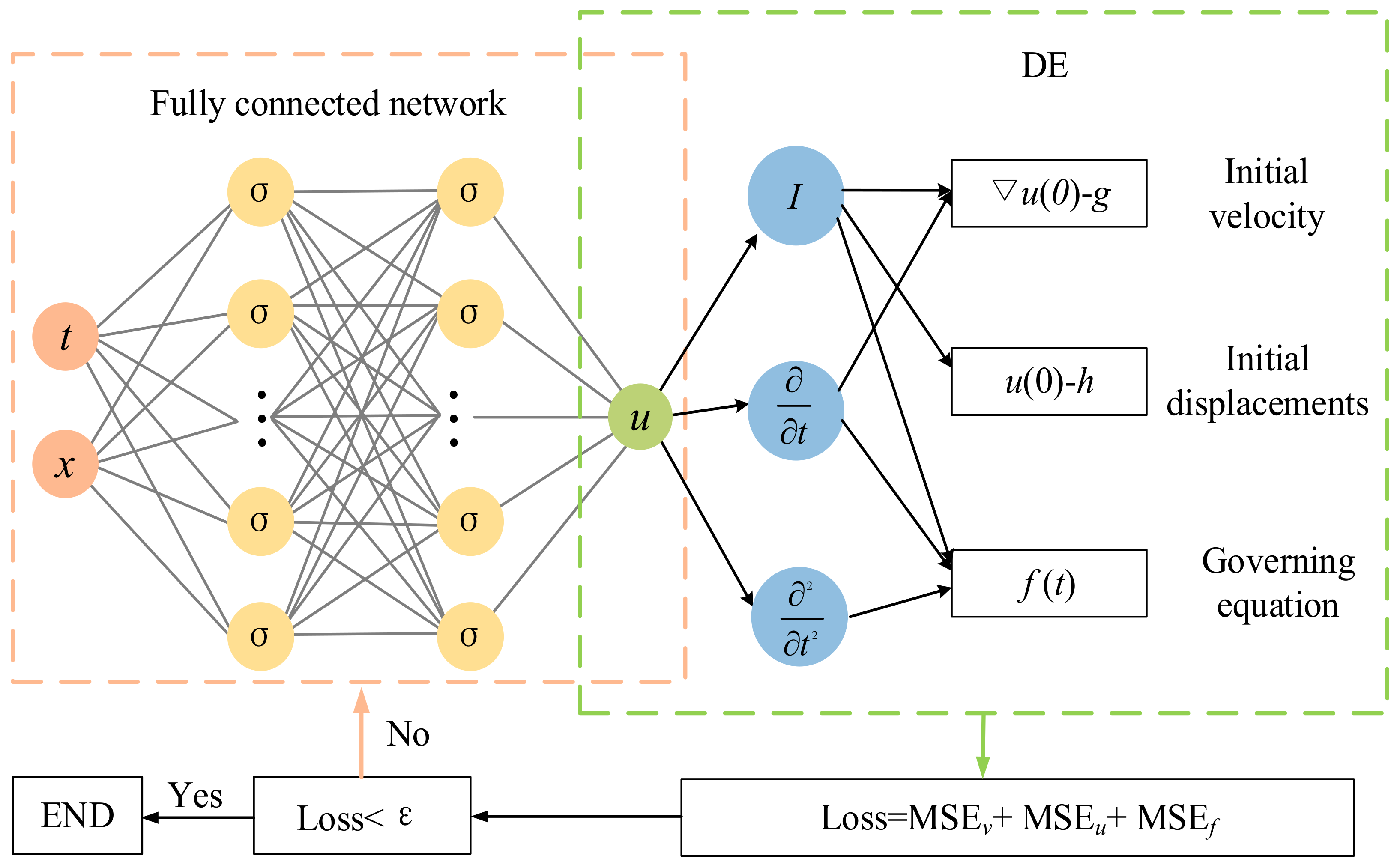
2. Physics-Informed Neural Networks

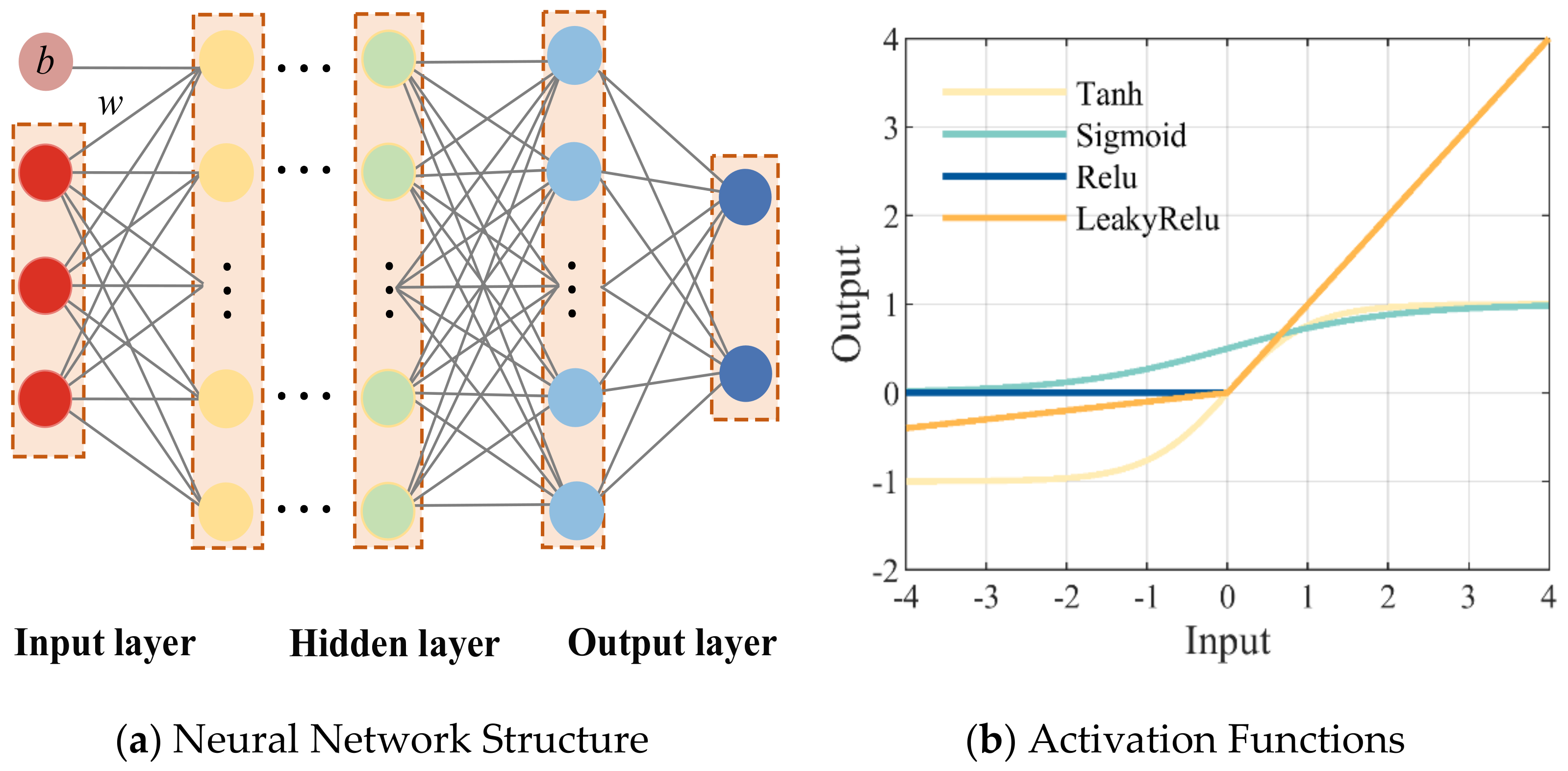
2.1. Fully Connected Neural Network

A neural network is a mathematical model that simulates the neural connections in the human brain for information processing. It approximates the real mapping relationship between input data and target output through information transmission among numerous neurons, nonlinear transformations by activation functions, and optimization algorithms for searching for optimal parameters. Essentially, it is a universal function approximator. When a neural network has enough depth (number of hidden layers) and width (number of neurons), it can approximate any continuous function with arbitrary precision. The basic components of a neural network include the input layer, output layer, hidden layer, weights, and biases, as shown in Figure 1a. The input layer receives input data and passes it to the hidden layer, with the number of nodes in the input layer determined by the features of the input data. The hidden layer performs a series of complex transformations and computations using the input data to learn the features and relationships within the data. The output layer is the last layer of the neural network, producing the output results, where the number of nodes is determined by the dimensions of the output results. At the connection of each layer in the neural network, there are weights and biases. Weights measure the importance of inputs and adjust the input data to better adapt to the feature relationships. Biases are constant values for each node and are used to adjust the thresholds of node outputs, enhancing the fitting capability and stability of the neural network to better accommodate different input data.

A neural network consists of multiple layers of neurons, where an activation function generates the output of each layer and serves as the input for the next layer. In this network, the output of each layer is determined by the previous layer’s results and the weights and biases of the neurons in that layer.

$${\mathit{l}}^{(i)}{=\mathit{w}}^{(i)}{\mathit{z}}^{(i-1)}+{\mathit{b}}^{(i)}$$

(1)

$${\mathit{z}}^{(i)}=\sigma ({\mathit{l}}^{(i)}), \forall \mathit{i}\in \{1,2,\cdots ,H\}$$

(2)

where $\sigma (·)$ is the activation function and ${\mathit{z}}^{(i)}$ and ${\mathit{z}}^{(i-1)}$ are the output vectors of the i − 1 and i-th layers, respectively. ${\mathit{w}}^{(i)}$ is the weight vector of the i-th layer and ${\mathit{b}}^{(i)}$ is the bias vector of the i-th layer.

Each neuron requires an activation function in the neural network to process input and output data. The activation function is crucial for learning and understanding highly complex and nonlinear functions. Its primary purpose is to introduce nonlinear transformations, enabling the neural network to learn nonlinearity and fit complex nonlinear function relationships. Common activation functions include the hyperbolic tangent function (tanh), logistic function (sigmoid), rectified linear unit function (ReLU), and leaky rectified linear unit function (LeakyReLU). Figure 1b shows the activation functions, and their definitions are provided in

Table 1. Activation functions.

Tanh	Sigmoid	ReLU	LeakyReLU
$\sigma (\mathit{z})={\displaystyle \frac{2}{1+e^{-2z}}}-1$	$\sigma (\mathit{z})={\displaystyle \frac{1}{1+{\mathit{e}}^{-z}}}$	$\sigma (z)=\left\{\begin{array}{l}max(0,z) ,z\ge 0\\ \hspace{1em}0 ,z<0\end{array}\right.$	$\sigma (z)=\left\{\begin{array}{l}{z}_i\hspace{1em}, \mathit{i}\mathit{f} \mathit{z}>0\\ a_i{z}_i, \mathit{i}\mathit{f} z\le 0\end{array}\right.$

.

2.2. Differential Equations

Many models in various fields can be described using differential equations. The solution of ordinary and partial differential equations is essential for many engineering fields. This paper uses the example of the equations of motion with N degrees of freedom and uses the PINN method to solve them. The equation of motion of an N-degree-of-freedom (DOF) damped structural system is given as follows:

$$\mathit{M}\ddot{\mathit{u}}(t)+\mathit{C}\dot{\mathit{u}}(t)+\mathit{K}\mathit{u}(t)=\mathit{F}$$

(3)

where M, C, and K are the $\mathit{N}\times \mathit{N}$ mass, damping, and stiffness matrices, respectively. F is the excitation force on the corresponding DOF of the system. The variables $\ddot{\mathit{x}}(t)$, $\dot{\mathit{x}}(t)$, and $\mathit{x}(t)$ are the $\mathit{N}\times 1$ displacement, velocity, and acceleration vectors, respectively.

For a more straightforward representation, the equation of motion can be expressed in a generalized form as follows:

$$\mathit{G}\left(t,\mathit{u}(t),\nabla \mathit{u}(t),\nabla {\mathit{u}}^2(t)\right)=0, t\in {\Omega }_t$$

(4)

$$\mathit{u}(t=0)=h$$

(5)

$$\nabla \mathit{u}(t=0)=g$$

(6)

In this equation, $u(t)$ represents the solution of the ordinary differential equation and $\nabla$ represents the differential operator. ${\Omega }_t$ corresponds to the temporal coordinates, and h and g denote the initial displacement and velocity, respectively. For convenience in the subsequent representation, let $f(t)=\mathit{G}\left(t,\mathit{u}(t),\nabla \mathit{u}(t),\nabla {\mathit{u}}^2(t)\right)$.

2.3. Training Process of Neural Network

A fully connected neural network is a data-driven neural network that can only uncover hidden features between input and output data. It is unable to consider the prior information between the data. Figure 2 shows the structure of the PINN, which allows for the embedding of physical equations, boundary conditions, and initial conditions into the training process. Adding a penalty term to the loss function jointly evaluates the difference between the model’s predicted output and the actual results, effectively preventing overfitting problems. The objective of the training process is to minimize the loss function. Choosing an appropriate loss function is crucial. This directly affects the training effectiveness and prediction performance of the neural network. The automatic differentiation technique [29] in deep neural networks provides convenience for embedding differential forms of physical information. This technique can automatically compute the derivatives or partial derivatives of functions without requiring the manual derivation or writing of differentiation expressions. The derivatives are calculated by combining the backpropagation algorithm and the chain rule, optimizing the computation process.

When using the PINN to approximate the solution of a differential equation $u_t(x^i,t^i)$, the loss function can be expressed as follows:

$$Loss=MS{E}_f+{\displaystyle \sum {\lambda }_{i}MS{E}_u}+{\displaystyle \sum {\lambda }_{j}MS{E}_v}$$

(7)

$$MS{E}_f={\displaystyle \frac{1}{N_f}}{\displaystyle \sum _{i=1}^{N_f}{\left|f(t^i)\right|}^2}$$

(8)

$$MS{E}_u={\displaystyle \frac{1}{N_u}}{\displaystyle \sum _{i=1}^{N_B}{\left|u\left(t^i\right)-h^i\right|}^2}$$

(9)

$$MS{E}_v={\displaystyle \frac{1}{N_v}}{\displaystyle \sum _{i=1}^{N_t}{\left|\nabla u\left(t^i\right)-g^i\right|}^2}$$

(10)

where $MS{E}_f$, $MS{E}_u$, and $MS{E}_v$ represent the loss terms for the governing equation, initial displacement, and initial velocity, respectively. ${\lambda }_i$ and ${\lambda }_j$ are the weight coefficients for the boundary and initial condition losses, respectively. They are used to balance the loss function for optimal performance. The choice of weight coefficients needs to be adjusted based on experience. $N_f$, $N_u$, and $N_v$ are the numbers of data points for different loss terms.

The training of the network involves the use of optimization algorithms and backpropagation to adjust the weights and biases of the neurons. The ultimate goal is to minimize the loss function and make the output of the PINN approximate the actual values. Commonly used optimization algorithms include stochastic gradient descent (SGD), AdaGrad, RMSprop, Adam, and L-BFGS. The Adam algorithm is a gradient-based optimization algorithm. This algorithm combines first- and second-moment estimates of the gradients and uses a decaying learning rate to train the network. In the early stages of training, a high learning rate enables fast searching. In the later stages, a low learning rate allows for more stable searching. This algorithm achieves faster convergence speed and greater stability by employing mini-batch data. The update strategy for Adam is as follows:

$$m_k\leftarrow {\beta }_1\times m_{k-1}+(1-{\beta }_1)\times \nabla g_k$$

(11)

$${\widehat{m}}_k\leftarrow {\displaystyle \frac{m_k}{1-{\beta }_1^k}}$$

(12)

$$v_k\leftarrow {\beta }_2\times v_{k-1}+(1-{\beta }_2)\times {\nabla }^2{g}_k$$

(13)

$${\widehat{v}}_k\leftarrow {\displaystyle \frac{v_k}{1-{\beta }_2^k}}$$

(14)

$${\theta }_{k+1}\leftarrow {\theta }_k+{\alpha }_k{\displaystyle \frac{{\widehat{m}}_k}{\sqrt{{\widehat{v}}_k}+\epsilon }}$$

(15)

where $\nabla g_k=\nabla Loss$ is the estimate of the gradient of the objective function at the k-th iteration. $m_k$ and $v_k$ represent the first and second moments of the gradient, respectively. ${\widehat{m}}_k$ and ${\widehat{v}}_k$ are used to correct the bias introduced by initializing the first- and second-moment estimates. ${\beta }_1$ and ${\beta }_2$ are the decay rates for the first- and second-moment estimates of the gradient, respectively. $\epsilon$ is a small value used to avoid division by zero. In this paper, the initial first- and second-moment estimates of the gradient are set to $m_0=0$ and $v_0=0$, respectively. The initial hyperparameters are set to ${\alpha }_0=0.01$, ${\beta }_1=0.9$, ${\beta }_2=0.999$, and $\epsilon ={10}^{-8}$.

By using optimization algorithms and backpropagation techniques, the goal is to minimize the loss function and obtain the optimal network parameter, ${\theta }^{\ast }$.

$${\theta }^{\ast }=\{\mathit{w},\mathit{b}\}=\arg \min {\displaystyle \frac{1}{N}}{\displaystyle \sum _{i=1}^{N}Loss}$$

(16)

3. Numerical Studies

The motion equation is a mathematical equation that describes the motion state of a structural system. The method typically involves the functional relationships between motion parameters such as position, velocity, and acceleration. This section presents three numerical examples of forced vibrations in damped multi-degree-of-freedom systems. The displacement response of the system is obtained by using the PINN to solve the differential equations of motion. The influence of network configuration on predictive performance is also analyzed in this section. The work in this paper is based on the MATLAB 2021b environment and uses a computer with an Intel CPU i7 12700 and 64 Gb of RAM.

3.1. Two-Degree-of-Freedom System

A damped two-degree-of-freedom model, as shown in Figure 3a, was selected to verify the accuracy of the proposed method. The mass, stiffness, and damping of each floor are 5 kg, 10 N/m, and 1 N·s/m, respectively. An external load P₁ is applied at the m₁ position on the first floor, as shown in Figure 3b. It is assumed that m₁ and m₂ only experience horizontal displacement without vertical movement. The motion state of the system can be represented by the displacement coordinates u₁ and u₂, which are the distances of masses m₁ and m₂ from their respective origin positions. The proposed method is used to compute the displacement response within 1 s. By analyzing the forces based on the principle of virtual work, the motion equation of the structure can be expressed as follows:

$$\left(\begin{array}{cc}{m}_1& 0\\ 0& m_2\end{array}\right)\left\{\begin{array}{c}{\ddot{u}}_1\\ {\ddot{u}}_2\end{array}\right\}+\left(\begin{array}{cc}{c}_1+c_2& -c_1\\ -c_2& c_2\end{array}\right)\left\{\begin{array}{c}{\dot{u}}_1\\ {\dot{u}}_2\end{array}\right\}+\left(\begin{array}{cc}{k}_1+k_2& -k_1\\ -k_2& k_2\end{array}\right)\left\{\begin{array}{c}{u}_1\\ u_2\end{array}\right\}=\left\{\begin{array}{c}{P}_1\\ 0\end{array}\right\}$$

(17)

Initial conditions:

$$u(t=0)=0, \dot{u}(t=0)=0, i=1,2$$

where $\dot{u}$ and $\ddot{u}$ are the velocity and displacement, which are the first and second derivatives of displacement $u$, respectively. m denotes the mass of the mass point, c represents the damping of the system, and k represents the stiffness. The system parameters are set as m₁ = m₂ = 5 kg, c₁ = c₂ = 1 N·s/m, and k₁ = k₂ = 10 N/m. The external load and time t satisfy P₁ = −sin(5 × t × π) × 1000 N. Let f represent the left-hand side of the motion equation.

The loss function of this model is expressed as follows:

$$Loss=Los{s}_1+{\lambda }_{1}Los{s}_u+{\lambda }_{2}Los{s}_v$$

(18)

$$Los{s}_1=MSE\left(f\left({\mathit{u}}_1\right),0\right)+MSE\left(f\left({\mathit{u}}_2\right),P_1\right)$$

(19)

$$Los{s}_u={\displaystyle \sum _i^{2}MSE\left({\mathit{u}}_i(0),0\right)}, Los{s}_v={\displaystyle \sum _i^{2}MSE\left({\dot{\mathit{u}}}_i(0),0\right)}$$

(20)

where $Los{s}_u$ and $Los{s}_v$ are the loss terms of the initial displacement and initial velocity, respectively, and ${\lambda }_1$ and ${\lambda }_2$ are the weighting coefficients for the initial conditions.

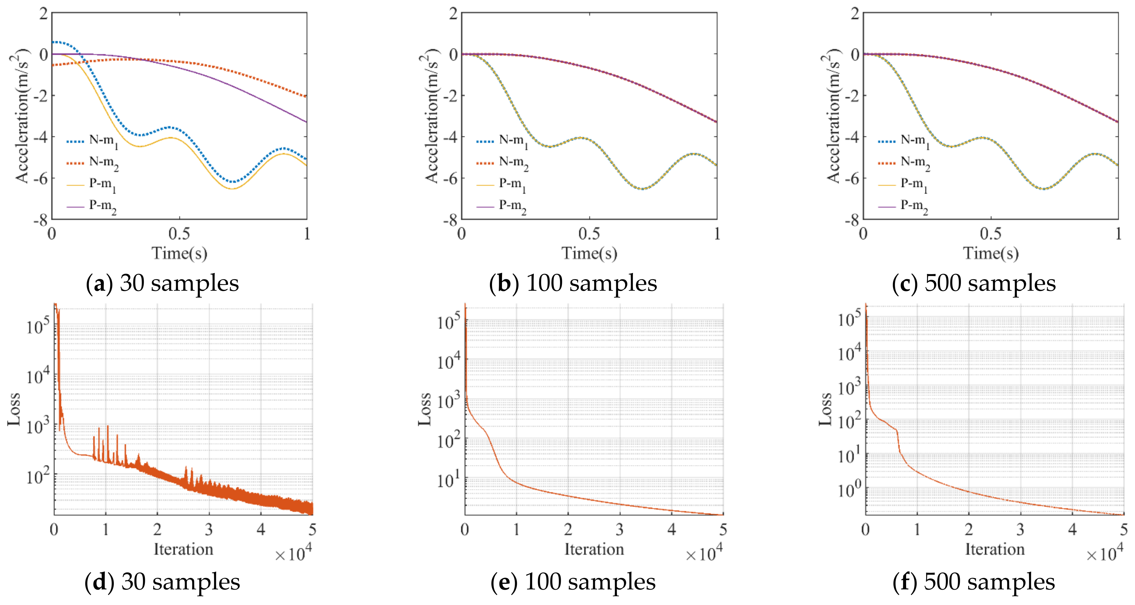
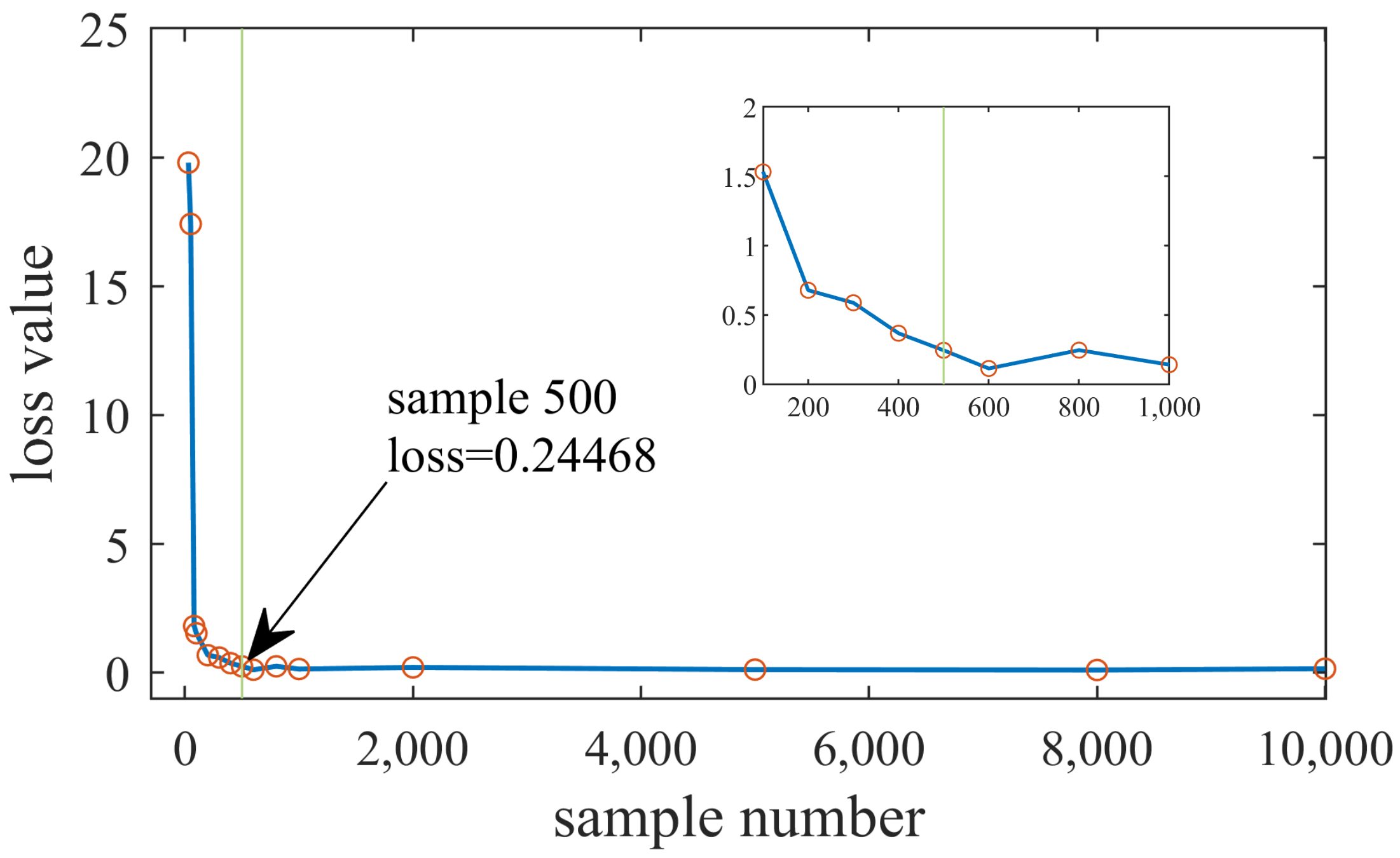
3.1.1. Training Sample Number

In this example, the PINN is used to predict the displacement response of the two-degree-of-freedom system. The convergence performance of the network is evaluated using different numbers of training samples. Input samples are randomly obtained within the interval $t\in [0,1]$ using the Sobol sequence. The weight coefficients ${\lambda }_1$ and ${\lambda }_2$ of the loss function are both set to 10. The network is configured with six hidden layers, each consisting of 20 neurons. The size of the input layer is 1, and the size of the output layer is 2. The activation function tanh is used. The Adam optimization algorithm executes 50,000 iterations to minimize the loss function. This example includes 15 different numbers of training samples, with the batch size set as one-tenth of the total training sample size, and we analyze the effect of training samples on the convergence of the PINN. The results obtained from calculations using the Newmark-β method are used as reference solutions. Due to the numerous cases, this paper only presents the prediction results and convergence process of the loss function for 30, 100, and 500 training samples, as shown in Figure 4, where “N” represents the results obtained using the Newmark-β method and “P” represents the results obtained using the PINN.

Figure 5 shows the loss values with iterations. When the number of training samples is less than 200, the loss function decreases rapidly as the training samples increase. As the number of training samples exceeds 200, the convergence speed gradually slows. When the number of training samples reaches 500, the loss function reaches a converged state. After that, with an increase in the number of samples, the final loss value shows no significant change. Cross-validation is used to estimate the prediction error of the model. Figure 6 shows the error variation generated over time by 500 training samples. The error represents the difference between the acceleration curves calculated numerically and by PINN. It can be observed that the maximum error for m₁ is only 0.0022, and for m₂, it is only 0.0014 throughout the entire time record. These values are significantly smaller than the acceleration at that moment, indicating that the errors are acceptable.

3.1.2. Number of Hidden Layers and Neurons

This section studies the predictive performance of the PINN under different numbers of hidden layers and neurons. The training set is generated using the Sobol sequence, and 500 training samples are generated. Figure 7 shows the convergence process of the loss function, where “Epochs” represents the number of training epochs. The specific configuration of the neural network is shown in

Table 2. Case settings and loss values.

Case	Active Function	Hidden Layers	Neurons	Loss Value
1	Tanh	2	10	5259.4248
2	Tanh	4	10	72.4586
3	Tanh	6	10	11.2092
4	Tanh	2	20	138.7688
5	Tanh	4	10	0.89231
6	Tanh	6	20	0.24468

, while the other parameters remain the same as in Section 3.1.1. When the number of hidden layers or neurons is too low, the constructed PINN tends to underfit, resulting in significant prediction errors. The number of hidden layers and neurons significantly affects the prediction results, and appropriately increasing the width and depth of the network can help improve the predictive performance.

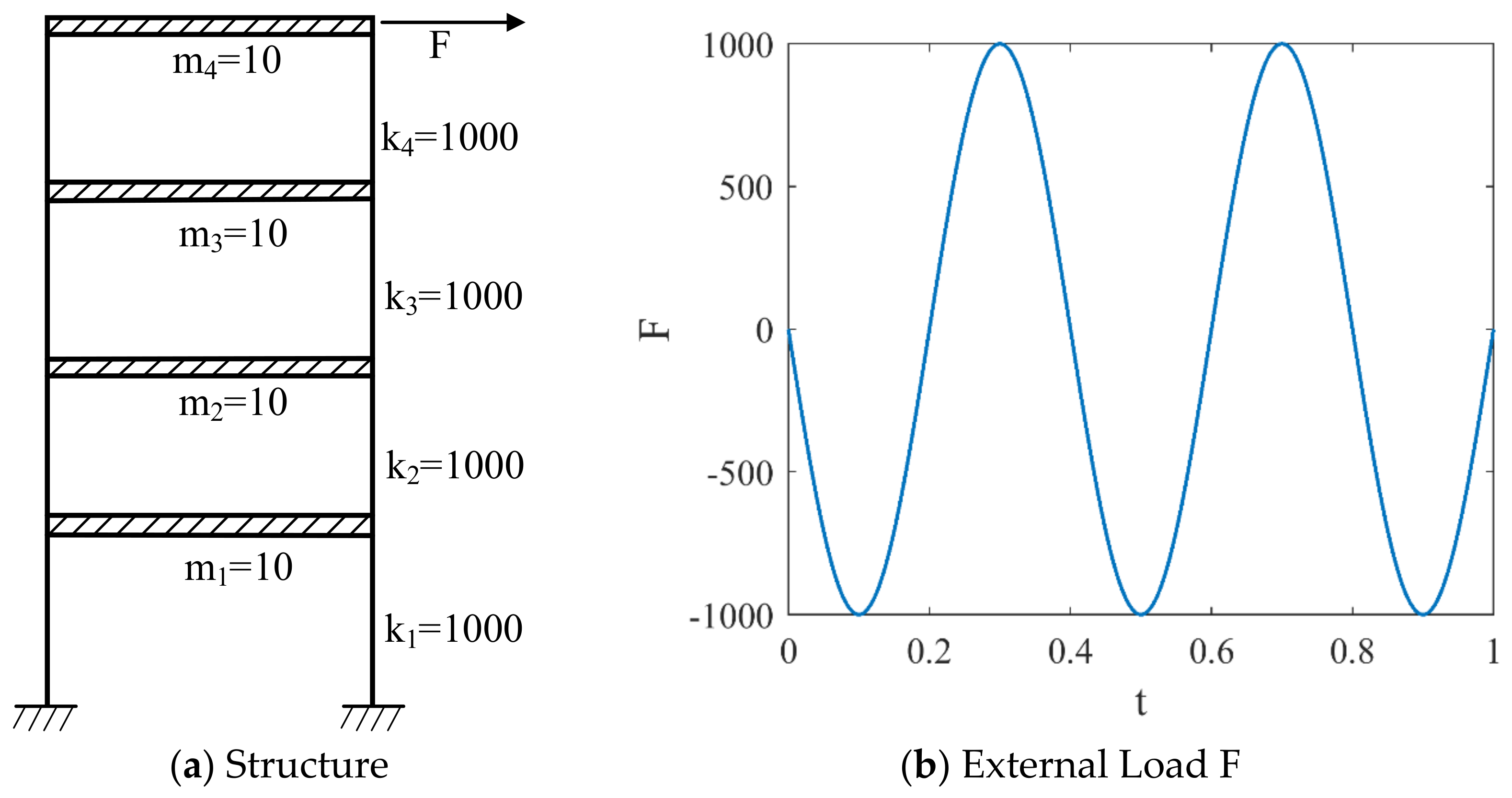
3.2. Four-Layer Framework Structure

A four-layer framework structure is subjected to external load excitation in this section to validate the effectiveness of the proposed method. The floor is assumed to be rigid, and the mass of the columns is neglected. The mass and stiffness of each floor are shown in Figure 8a. The mass and stiffness of each floor are 10 t and 1000 kN/m, respectively. Rayleigh damping is used in this case, with a damping ratio of 5%, and the damping coefficient is obtained from the first two natural frequencies. It is assumed that the system’s mass is mainly concentrated on the floors, and the external load F(t) is applied at the top of the structure. The form of the external load F(t) is shown in Figure 8b, and the displacement response of each floor within 1 s is analyzed. According to the D’Alembert principle, for a multi-degree-of-freedom structure subjected to external load action, the equation of motion can be expressed as follows:

$$M\ddot{u}(t)+C\dot{u}(t)+Ku(t)=F(t).$$

(21)

In the equation, M, C, and K represent the mass, damping, and stiffness matrices, respectively. The system utilizes Rayleigh damping with a damping ratio of 5%. $F(t)$ is the external load, following the function $F(t)=-\sin (5\pi \times t)\times 1000$ kN.

The loss function considers the initial conditions of displacement and velocity. Therefore, the loss function for this numerical example can be expressed as follows:

$$Loss=Los{s}_1+{\lambda }_1{\displaystyle \sum _{\mathrm{i}=1}^{4}Los{s}_u(u_i(0),0)}+{\lambda }_2{\displaystyle \sum _{i=1}^{4}Los{s}_v({\dot{u}}_i(0),0)}.$$

(22)

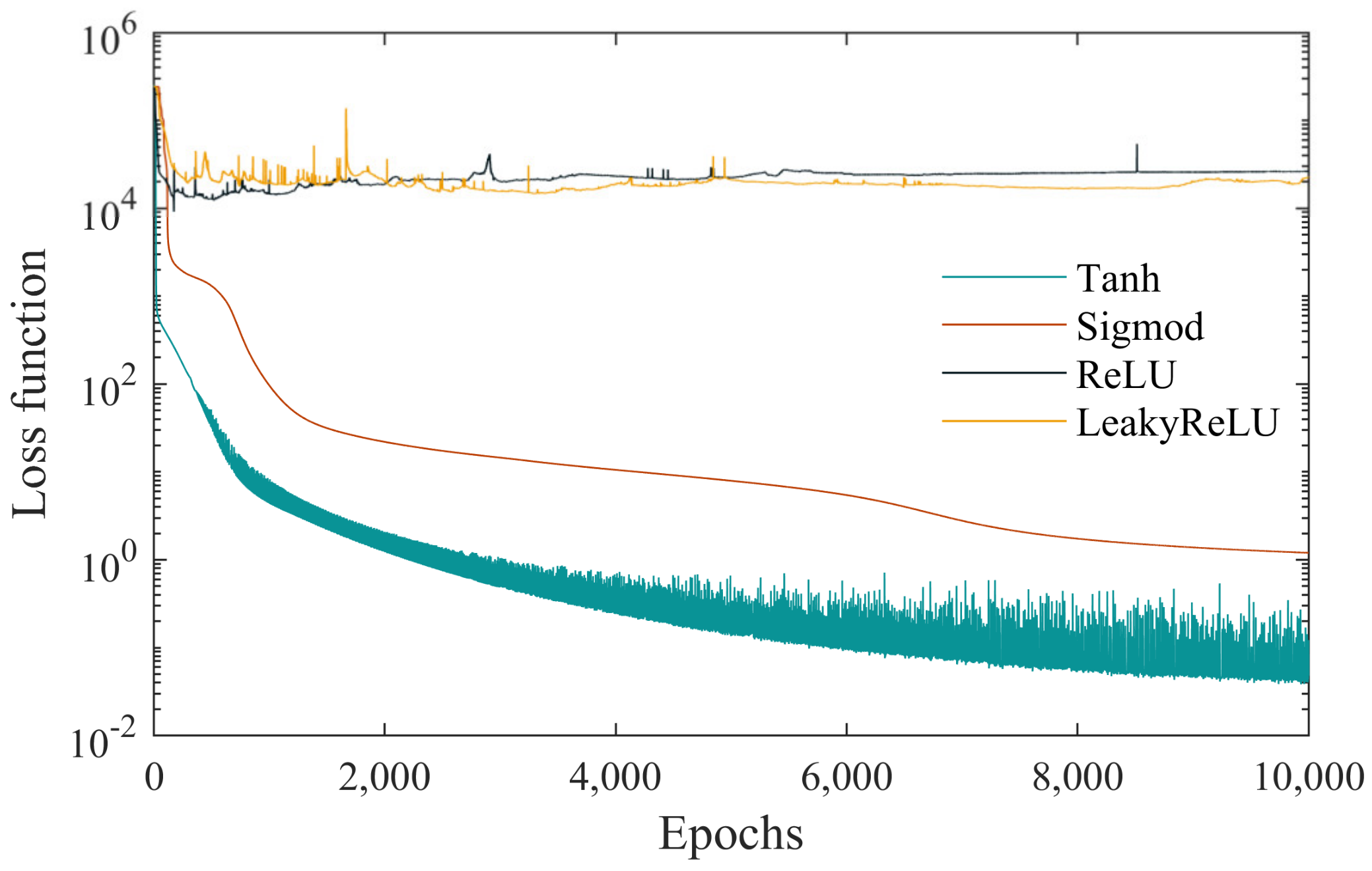
3.2.1. Activation Function

In this section, the prediction performances of four activation functions are studied: tanh, sigmoid, ReLU, and LeakyReLU. The PINN is set up with eight hidden layers, and each layer contains 20 neutrons. The optimization algorithm and sampling method are consistent with those in Section 3.1. The network is trained using 3000 samples, with batch sizes of 300 and 10,000 epochs. The weight coefficients ${\lambda }_1$ and ${\lambda }_1$ of the loss function are both 10. The output layer of the network is set to have four nodes, representing the output channels for the displacement of four degrees of freedom. The iterative results of the loss function are shown in Figure 9.

Figure 10 shows the prediction results of the PINN. The solid line represents the computational results obtained using the Newmark-β method, while the dashed line represents the prediction results of the PINN. When the tanh function is used as the activation function, the constructed PINN achieves the best predictive performance, consistent with the reference solution. However, ReLU and LeakyReLU have poor learning capabilities, possibly due to the involvement of differential operations in the PINN. The ReLU and LeakyReLU functions have discontinuous derivatives, which hinder the training of certain parameters, leading to nonconvergence or convergence to local minima with significant errors. The predictive performance of the PINN greatly relies on accurately evaluating the derivatives of the activation function.

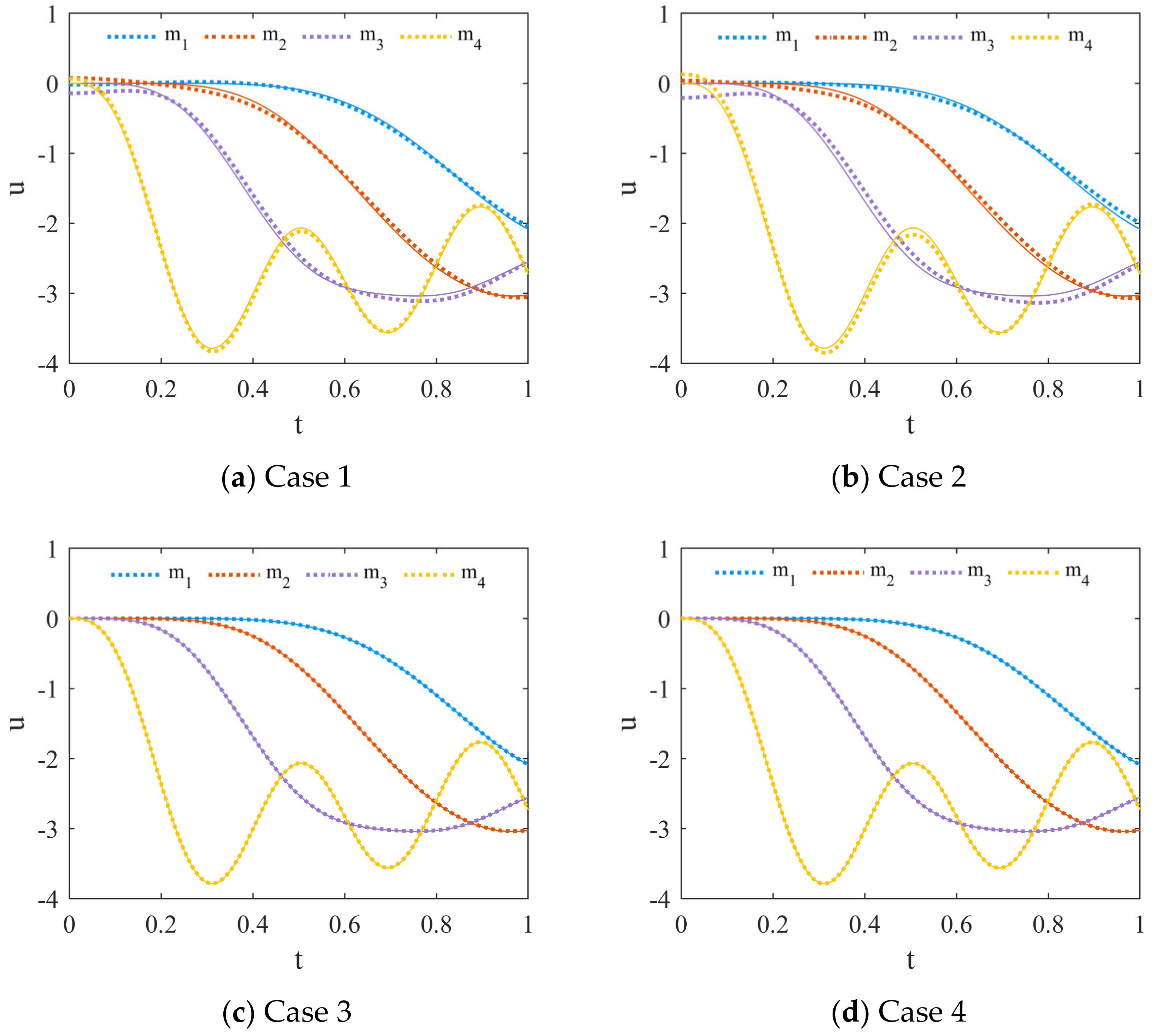
3.2.2. The Weight Coefficients of the Loss Function

The loss function comprises various loss terms, including control equations, initial conditions, and boundary conditions. The predictive accuracy of the PINN is sensitive to the weight coefficients of these loss terms. Therefore, in this section, the prediction results of the PINN under different weight coefficients of loss function terms are analyzed, and the neural network’s parameter settings are shown in

Table 3. The neural network parameters.

Case	Hidden Layers	Neuron Nodes	Active Function	${\mathit{\lambda }}_1$	${\mathit{\lambda }}_2$
1	8	20	Tanh	1	1
2	8	20	Tanh	1	1000
3	8	20	Tanh	1000	1
4	8	20	Tanh	1000	1000

.

Figure 11 shows the comparison results, with the dashed line representing the predictions of the PINN and the solid line representing the reference values. In Case 1 and Case 2, there is a larger error at t = 0, indicating that the loss term corresponding to the initial velocity has a minor impact on the prediction results. The results of Case 1 and Case 3 demonstrate that changing the weighting coefficient ${\lambda }_2$, corresponding to the initial displacement, can significantly improve the prediction results. The prediction results of Case 4 are consistent with the reference solution, showing the best predictive performance. Therefore, achieving good predictive performance requires selecting reasonable weighting coefficients to balance the impact of each term in the loss function.

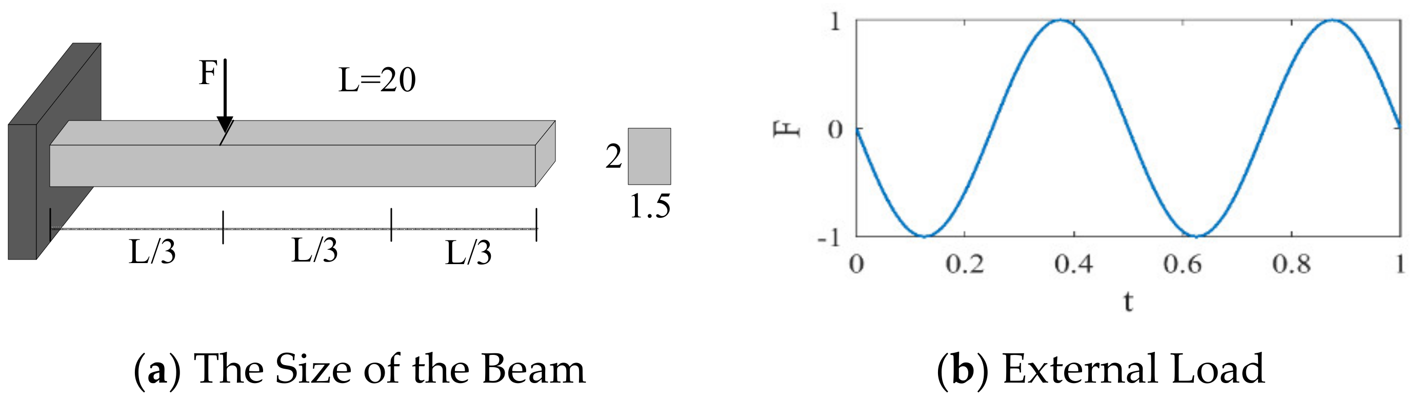
3.3. Cantilever Beam

In this section, a linear cantilever beam structure is used to verify the effectiveness of the proposed PINN. The length of the cantilever beam (L) is 20. The cross-sectional dimensions (b × h) are 1.5 × 2, and the cross-sectional area (A) is three square units. The beam is discretized into three elements, with each node having two degrees of freedom. Assuming that the cantilever beam is made of a linear elastic material, the density (ρ) is 50, and the flexural stiffness (E) is 1 × 10⁵. The damping matrix is constructed using Rayleigh damping. The left end of the beam is fixed, and an external load is applied at a distance of L/3 from the fixed end. The load (F) is a function of time (t) and can be expressed as F = −sin(4π × t), as shown in Figure 12b. The values given in this case are in consistent units. The displacement of each DOF is solved using the proposed PINN method, with the solution from the Newmark-β method used as a reference solution.

The form of the motion equation for the structure is consistent with that in Section 3.2. The loss function is defined as follows:

$$Loss=Los{s}_1+{\lambda }_1{\displaystyle \sum _{i=1}^6{Los{s}_u}^{(i)}}+{\lambda }_2{\displaystyle \sum _{i=1}^6{Los{s}_v}^{(i)}}$$

(23)

In this example, the PINN is used for analyzing the displacement response of a structure. The neural network is employed as a function solver to compute the solutions for the motion differential equations. The network uses the Sobol sequence method to generate 3000 samples trained using the Adam algorithm with batch sizes of 300 and 80,000 epochs. The hyperparameters of the neural network are obtained by minimizing the loss function that incorporates physical information. In this case, the weight coefficients ${\lambda }_1$ and ${\lambda }_2$ of the loss function terms are both set to 100. The input layer has a size of 1, and the output layer represents the displacement response of the six DOFs. The activation function used is Tanh. The network is configured with 10 hidden layers, each containing 20 neurons. Figure 13 displays the convergence process of the loss function, with a final loss value of 1.0528 × 10⁻⁴. Figure 14 presents the prediction results of the PINN. The solid line represents the reference solution, while the dashed line represents the predicted results. The predicted results closely match the reference solution, indicating that the PINN exhibits excellent predictive performance.

4. Conclusions

This paper presents a neural network method grounded in physical principles to solve differential equations of motion, and specifically examines the application of physics-informed neural networks (PINNs) in the analysis of forced motion in multi-degree-of-freedom systems with damping. The governing equations for the structural system were derived using the principles of virtual work and D’Alembert’s principle. Physical constraints, such as boundary and initial conditions, were embedded into the loss function through automatic differentiation techniques. A Sobol sequence was utilized to generate the sample set, while the Adam optimization algorithm was employed to minimize the loss function and optimize the neural network’s weights and biases. The developed PINN model, which is consistent with physical laws, was then applied to solve the differential equations. Three numerical examples—a two-degree-of-freedom system, a four-layer frame structure, and a cantilever beam—were analyzed, to investigate the influence of input samples, activation functions, loss function weight coefficients, and the neural network’s width and depth on the predictive performance of the PINN. The results demonstrate that the proposed PINN method effectively solves differential equations of motion for forced vibrations in damped systems. When the number of layers in a neural network is too small, the response of the estimated output cannot be accurately modelled. The number of neural network layers is recommended to be set at four to five layers. Too many will result in more hyper elaboration to be identified and optimized and will increase the computation time. By appropriately selecting network parameters, this approach can be generalized for solving differential equations. In future studies, we will use this method for the analysis of complex structures.

References

1. Farlow, S.J. Partial Differential Equations for Scientists and Engineers; Courier Corporation: Chelmsford, MA, USA, 1993. [Google Scholar]
2. Ames, W.F. Numerical Methods for Partial Differential Equations; Academic Press: Cambridge, MA, USA, 2014. [Google Scholar]
3. Johnson, C. Numerical Solution of Partial Differential Equations by the Finite Element Method; Courier Corporation: Chelmsford, MA, USA, 2012. [Google Scholar]
4. Smith, G.D.; Smith, G.D.; Smith, G.D.S. Numerical Solution of Partial Differential Equations: Finite Difference Methods; Oxford University Press: Oxford, UK, 1985. [Google Scholar]
5. Belytschko, T.; Schoeberle, D. On the unconditional stability of an implicit algorithm for nonlinear structural dynamics. J. Appl. Mech. 1975, 42, 865–869. [Google Scholar] [CrossRef]
6. Ijari, K.; Paternina-Arboleda, C.D. Sustainable Pavement Management: Harnessing Advanced Machine Learning for Enhanced Road Maintenance. Appl. Sci. 2024, 14, 6640. [Google Scholar] [CrossRef]
7. Feretzakis, G.; Sakagianni, A.; Anastasiou, A.; Kapogianni, I.; Tsoni, R.; Koufopoulou, C.; Karapiperis, D.; Kaldis, V.; Kalles, D.; Verykios, V.S. Machine Learning in Medical Triage: A Predictive Model for Emergency Department Disposition. Appl. Sci. 2024, 14, 6623. [Google Scholar] [CrossRef]
8. Li, Q.; Ni, P.; Du, X.; Han, Q.; Xu, K.; Bai, Y. Bayesian finite element model updating with a variational autoencoder and polynomial chaos expansion. Eng. Struct. 2024, 316, 118606. [Google Scholar] [CrossRef]
9. Ni, P.; Han, Q.; Du, X.; Fu, J.; Xu, K. Probabilistic model updating of civil structures with a decentralized variational inference approach. Mech. Syst. Signal Process. 2024, 209, 111106. [Google Scholar] [CrossRef]
10. Michoski, C.; Milosavljević, M.; Oliver, T.; Hatch, D.R. Solving differential equations using deep neural networks. Neurocomputing 2020, 399, 193–212. [Google Scholar] [CrossRef]
11. Lagaris, I.E.; Likas, A.; Fotiadis, D.I. Artificial neural networks for solving ordinary and partial differential equations. IEEE Trans. Neural Netw. 1998, 9, 987–1000. [Google Scholar] [CrossRef] [PubMed]
12. Rudd, K.; Ferrari, S. A constrained integration (CINT) approach to solving partial differential equations using artificial neural networks. Neurocomputing 2015, 155, 277–285. [Google Scholar] [CrossRef]
13. Piscopo, M.L.; Spannowsky, M.; Waite, P. Solving differential equations with neural networks: Applications to the calculation of cosmological phase transitions. Phys. Rev. D 2019, 100, 016002. [Google Scholar] [CrossRef]
14. Berg, J.; Nyström, K. A unified deep artificial neural network approach to partial differential equations in complex geometries. Neurocomputing 2018, 317, 28–41. [Google Scholar] [CrossRef]
15. Karniadakis, G.E.; Kevrekidis, I.G.; Lu, L.; Perdikaris, P.; Wang, S.; Yang, L. Physics-informed machine learning. Nat. Rev. Phys. 2021, 3, 422–440. [Google Scholar] [CrossRef]
16. Ding, Y.; Ye, X.-W. Fatigue life evolution of steel wire considering corrosion-fatigue coupling effect: Analytical model and application. Steel Compos. Struct. 2024, 50, 363–374. [Google Scholar]
17. Zhang, S.; Ni, P.; Wen, J.; Han, Q.; Du, X.; Xu, K. Automated vision-based multi-plane bridge displacement monitoring. Autom. Constr. 2024, 166, 105619. [Google Scholar] [CrossRef]
18. Li, Q.; Du, X.; Ni, P.; Han, Q.; Xu, K.; Yuan, Z. Efficient Bayesian inference for finite element model updating with surrogate modeling techniques. J. Civ. Struct. Health Monit. 2024, 14, 997–1015. [Google Scholar] [CrossRef]
19. Li, Q.; Du, X.; Ni, P.; Han, Q.; Xu, K.; Bai, Y. Improved hierarchical Bayesian modeling framework with arbitrary polynomial chaos for probabilistic model updating. Mech. Syst. Signal Process. 2024, 215, 111409. [Google Scholar] [CrossRef]
20. Zhang, W.; Zhao, M.; Du, X.; Gao, Z.; Ni, P. Probabilistic machine learning approach for structural reliability analysis. Probabilistic Eng. Mech. 2023, 74, 103502. [Google Scholar] [CrossRef]
21. Ding, Y.; Ye, X.-W.; Guo, Y. Copula-based JPDF of wind speed, wind direction, wind angle, and temperature with SHM data. Probabilistic Eng. Mech. 2023, 73, 103483. [Google Scholar] [CrossRef]
22. Raissi, M.; Perdikaris, P.; Karniadakis, G.E. Physics-informed neural networks: A deep learning framework for solving forward and inverse problems involving nonlinear partial differential equations. J. Comput. Phys. 2019, 378, 686–707. [Google Scholar] [CrossRef]
23. Haghighat, E.; Raissi, M.; Moure, A.; Gomez, H.; Juanes, R. A physics-informed deep learning framework for inversion and surrogate modeling in solid mechanics. Comput. Methods Appl. Mech. Eng. 2021, 379, 113741. [Google Scholar] [CrossRef]
24. Wei, S.; Jin, X.; Li, H. General solutions for nonlinear differential equations: A rule-based self-learning approach using deep reinforcement learning. Comput. Mech. 2019, 64, 1361–1374. [Google Scholar] [CrossRef]
25. Cai, S.; Wang, Z.; Wang, S.; Perdikaris, P.; Karniadakis, G.E. Physics-informed neural networks for heat transfer problems. J. Heat Transf. 2021, 143, 060801. [Google Scholar] [CrossRef]
26. Meng, X.; Li, Z.; Zhang, D.; Karniadakis, G.E. PPINN: Parareal physics-informed neural network for time-dependent PDEs. Comput. Methods Appl. Mech. Eng. 2020, 370, 113250. [Google Scholar] [CrossRef]
27. Yang, L.; Meng, X.; Karniadakis, G.E. B-PINNs: Bayesian physics-informed neural networks for forward and inverse PDE problems with noisy data. J. Comput. Phys. 2021, 425, 109913. [Google Scholar] [CrossRef]
28. Bolandi, H.; Sreekumar, G.; Li, X.; Lajnef, N.; Boddeti, V.N. Physics Informed Neural Network for Dynamic Stress Prediction. arXiv 2022, arXiv:2211.16190. [Google Scholar] [CrossRef]
29. Baydin, A.G.; Pearlmutter, B.A.; Radul, A.A.; Siskind, J.M. Automatic differentiation in machine learning: A survey. J. Marchine Learn. Res. 2018, 18, 1–43. [Google Scholar]
Figure 1. Fully Connected Neural Network.
Applsci 14 07694 g001
Figure 2. Structural diagram of PINN.
Applsci 14 07694 g002
Figure 3. Two-degree-of-freedom system.
Applsci 14 07694 g003
Figure 4. Partial analysis results.
Applsci 14 07694 g004
Figure 5. The convergence process of the loss function values.
Applsci 14 07694 g005
Figure 6. Error variation over time for m1 and m2.
Applsci 14 07694 g006
Figure 7. Loss function iteration results.
Applsci 14 07694 g007
Figure 8. Four-layer framework structure.
Applsci 14 07694 g008
Figure 9. Loss function iteration results.
Applsci 14 07694 g009
Figure 10. The predictive results of the PINN.
Applsci 14 07694 g010
Figure 11. Results of the PINN under different weight coefficients.
Applsci 14 07694 g011
Figure 12. Numerical example of a cantilever beam.
Applsci 14 07694 g012
Figure 13. Loss function.
Applsci 14 07694 g013
Figure 14. Predicted results of PINN.
Applsci 14 07694 g014