Article

Applications and Prospects of Smooth Particle Hydrodynamics in Tunnel and Underground Engineering

School of Civil Engineering, Beijing Jiaotong University, Beijing 100044, China
*
Author to whom correspondence should be addressed.
Appl. Sci. 2024, 14(18), 8552; https://doi.org/10.3390/app14188552
Submission received: 26 July 2024 / Revised: 14 September 2024 / Accepted: 18 September 2024 / Published: 23 September 2024

Abstract

:
Smoothed particle hydrodynamics (SPH) is a state-of-the-art numerical simulation method in fluid mechanics. It is a novel approach for modeling and comprehending complex fluid behaviors. In contrast to traditional grid-dependent techniques like finite element and finite difference methods, SPH utilizes a meshless, purely Lagrangian approach, offering significant advantages in fluid simulations. By leveraging a set of arbitrarily distributed particles to represent the continuous fluid medium, SPH enables the precise estimation of partial differential equations. This grid-free methodology effectively addresses many challenges associated with conventional methods, providing a more adaptable and efficient solution framework. SPH’s versatility is evident across a broad spectrum of applications, ranging from advanced computational fluid dynamics (CFD) to complex computational solid mechanics (CSM), and proves effective across various scales—from micro to macro and even astronomical phenomena. Although SPH excels in tackling problems involving multiple degrees of freedom, complex boundaries, and large discontinuous deformations, it is still in its developmental phase and has not yet been widely adopted. As such, a thorough understanding and systematic analysis of SPH’s foundational theories are critical. This paper offers a comprehensive review of the defining characteristics and theoretical foundations of the SPH method, supported by practical examples derived from the Navier–Stokes (N-S) equations. It also provides a critical examination of successful SPH applications across various fields. Additionally, the paper presents case studies of SPH’s application in tunnel and underground engineering based on practical engineering experiences and long-term on-site monitoring, highlighting SPH’s alignment with real-world conditions. The theory and application of SPH have thus emerged as highly dynamic and rapidly evolving research areas. The detailed theoretical analysis and case studies presented in this paper offer valuable insights and practical guidance for scholars and practitioners alike.

1. Introduction

Recent advancements in numerical simulation technologies have significantly impacted tunneling and underground engineering. As a mesh-free technique, smoothed particle hydrodynamics (SPH) offers significant advantages in addressing issues with mobile boundaries, especially those involving extensive deformations and intricate free-surface interactions. Based on current research findings, both domestically and internationally, SPH is predominantly applied in the following fields: celestial mechanics, explosive phenomena, high-velocity impact science, mining engineering, and fluid dynamics. The method’s broad application is largely due to its ability to incorporate constitutive equations that align with the properties of various materials. Furthermore, the existing literature strongly suggests that SPH has immense potential for future developments in tunnel and underground engineering.
Monaghan Sun, X and Tang, Y et al. [1,2,3] have highlighted the growing importance of meshless methods and computational fluid dynamics (CFD) in tackling intricate engineering problems. Cheng Y. et al. [4] underscored that meshless methods, which do not rely on grid structures, offer remarkable adaptability when managing complex boundary conditions and significant deformations, particularly in tunnel excavation and associated large-scale ground deformations. In contrast, Zhilang Z., Moubin L., and Hideto N. et al. [5,6,7,8] have pointed out that traditional finite element methods (FEM) and finite difference methods (FDM), which depend on predefined mesh structures, often face challenges such as mesh distortion and diminished computational accuracy during large-deformation simulations. Wijesooriya et al. [9] provided an extensive technical review of CFD applications in high-rise buildings and structures, while Tu et al. [10] utilized CFD models to analyze flow fields around bridge piers and study bridge scour. Tahir A., Tait S., and Chun Hwa C. et al. [11,12,13,14] argued that advancements in computational resources have facilitated the integration of CFD and meshless methods, enhancing the accuracy and stability of numerical simulations under complex conditions. Furthermore, Wang X. et al. [15] emphasized that alternative meshless methods, such as the meshless Galerkin method (EFG) and the discrete element method (DEM), have the potential to model complex stress–strain relationships and nonlinear boundary conditions, though they still encounter issues related to computational efficiency and precise parameter determination in practical engineering applications. Xiong et al. [16] proposed a CFD-based simulation approach that employs dynamic grid updating techniques and explores the effects of pier-type bridges on scour behavior. These advancements are anticipated to further advance the use of meshless methods and CFD in tunneling and underground engineering, thereby enhancing their practical value across various fields [17,18,19].
SPH was initially conceived to address astrophysical challenges within three-dimensional open space, with a particular focus on variability problems. Given that the movement of these particles mimics that of liquids or gases, they can be accurately described using the governing equations of classical Newtonian fluid dynamics. Related research on this topic was first seen in the relevant literature of JJ Monaghan [1]. Figure 1 shows a planetary synthesis process simulated by SPH. Ongoing problems such as galaxy and star formation, binary interactions, comet and asteroid impacts, and the dynamics of self-gravitational disks can be addressed.
Lian et al. [20] addressed the challenge of simulating the coupling of large deformations and failure in porous materials using the smoothed particle hydrodynamics (SPH) method. Peng et al. [21] introduced a numerical approach that integrates discontinuous deformation analysis (DDA) with SPH to model interactions between rock structures and soil particles. Hu et al. [22] employed a shear failure model combined with a contact algorithm to simulate the cutting process and interactions between tools and both non-cohesive and cohesive soils. During the discretization of the continuum, Chakraborty and Shaw [23] formulated an efficient interaction among immediate neighbors by incorporating a spring-like connection between discrete particles. The degradation of these spring forces is governed by a material damage evolution law. When the impact velocity increases, a similar sequence of failures is observed: tensile tearing at the support occurs at 40 m/s, and shear failure is evident at the impact site at 60 m/s (Figure 2).
Tao C. et al. [24] argued that SPH, with its Lagrangian framework and meshless nature, is becoming a prominent method in tunneling and underground engineering applications. Beyabanaki and Shintate, K. et al. [25,26,27,28] suggested that SPH excels in handling complex phenomena such as free-surface and multiphase flows, making it particularly useful for simulations involving soil excavation and ground deformation in recent studies. He et al. [29] validated the stability and accuracy of the SPH method in analyzing water–soil coupling interactions during dam seepage processes and underwater landslides through experiments utilizing a novel water–soil coupling wall boundary model.
As illustrated in Figure 3, several key moments (t = 0 s, t = 125 s, t = 500 s, and t = 1156 s) were chosen for analysis. Initially, the seepage velocity is high due to the dam’s low water content. By approximately 125 s, the water front has advanced to a position near x = 0.8 m. As the process continues and soil saturation increases, the seepage velocity decreases gradually. By around 500 s, the water front reaches approximately x = 1.2 m. At about 1156 s, the seepage process concludes, stabilizing at a steady state. These findings are consistent with the actual seepage process and provide preliminary evidence supporting the SPH method’s effectiveness in simulating seepage behavior. Despite these advancements, significant limitations remain in simulating large-deformation problems in tunnels and underground engineering, particularly regarding computational efficiency and model accuracy. To address these issues, researchers have proposed combining meshless methods with computational fluid dynamics (CFD) to enhance simulation accuracy and efficiency in complex tunnel environments [30,31,32,33]. This approach integrates SPH with CFD to refine smoothing length calculations, thereby improving model stability and convergence in large-deformation and multiphase flow scenarios [34,35]. To investigate fluid–solid interactions related to water and mud inrush during tunnel construction, Xia et al. [36] developed a coupled discontinuous SPH method. Numerical simulations and case studies have validated the effectiveness of this method in tunnel excavation and related ground-deformation issues, offering valuable theoretical insights for future engineering applications [37,38,39].
Although the smoothed particle hydrodynamics (SPH) method is well suited for the numerical simulation of large deformations in soft rock and mechanical cutting in hard rock within tunnel and underground engineering, several challenges limit its broader application. These challenges stem from the complexity of constitutive models for surrounding rock materials, the rheological characteristics of tunnel structures, and the spatiotemporal effects inherent in the tunnel excavation process. Notably, the current derivation of the fundamental theory behind the SPH method remains significantly underdeveloped, particularly under multi-field coupling conditions. Moreover, issues related to the definition of boundary conditions further constrain the use of SPH in tunnel and underground engineering, where its application is still in the early stages. This paper systematically summarizes and derives the key characteristics and fundamental equations of the SPH method, illustrating its application with an example based on the Navier–Stokes (N-S) equations. Furthermore, it provides an in-depth analysis of successful SPH applications across various fields. To enhance boundary representation and tensor stability, particularly in the context of tunneling, the SPH method is employed to simulate tunnel blasting construction. The simulation results show a strong correlation with actual monitoring data, offering robust theoretical guidance and practical insights for scholars in the field.

2. Characteristics, Principles, and a Case Study of SPH

2.1. Characteristics of SPH

The smoothed particle hydrodynamics (SPH) method is built upon three core components: smoothing, particles, and fluid dynamics. In this framework, “smoothing” involves the stable and continuous approximations derived from the weighted averaging of adjacent particles, enabling a fluid-like behavior in simulations. The term “particles” signifies a meshless representation system, wherein each particle embodies a discrete element of the simulated domain. “Fluid dynamics” refers to the primary application for which the SPH method has been specifically developed and refined. Compared to conventional grid-based techniques, the SPH method presents three unique advantages:
(1)
Meshless: The problem domain is entirely represented by particles, which act as the fundamental computational units for estimating field variables. This particle-based approach removes the necessity for grid-based partitioning, thereby sidestepping the challenges related to mesh distortion and reconstruction.
(2)
Adaptive: The kernel approximation of the field function is recalculated at each time step using all particles within the continuous domain. This adaptability ensures that the SPH method maintains robustness and consistency, even with arbitrary variations in particle distribution over time.
(3)
Lagrangian Integration: The SPH method seamlessly integrates Lagrangian properties with particle characteristics. Through the application of particle approximation techniques to discrete partial differential equations formulated in the Lagrangian framework—encompassing essential variables like velocity, density, and energy—the method establishes a coherent and precise system for capturing fluid dynamics.
The unique integration of meshless, adaptive, and Lagrangian characteristics renders the smoothed particle hydrodynamics (SPH) method a compelling alternative to conventional mesh-based approaches, especially in contexts characterized by significant deformation. This method’s versatility and robustness allow it to excel in simulating intricate fluid dynamics scenarios with both accuracy and efficiency. In contrast to other mesh-free techniques, where nodes serve merely as interpolation points, SPH particles intrinsically embody both material properties and computational elements. Functioning as both approximation locations and material constituents, these particles endow the SPH method with exceptional flexibility, facilitating the precise modeling and simulation of fluid dynamics. As a result, the SPH method finds widespread application across diverse domains of scientific research and engineering practice. The benefits of the SPH method encompass the following:
(1)
It is a mesh-free framework that demonstrates resilience to distortion and deformation.
(2)
It has high adaptability, making it suitable for scenarios with evolving boundaries.
(3)
The elimination of extensive element divisions effectively mitigates errors associated with local approximations found in finite element methods (FEMs).
(4)
There is continuity of the field function and its gradient within the solution domain, achieved through kernel function interpolation.
(5)
The resolution of governing equations is simplified, thereby easing the integration of chemical and thermodynamic effects.

2.2. Principles of SPH

The theoretical basis of smoothed particle hydrodynamics (SPH) stems from the particle method, which employs a collection of discrete particles to represent continuous physical quantities. This framework allows for numerical analysis through particle-based interpolation. In the SPH approach, the essential equations of fluid mechanics are converted into computational expressions via kernel function evaluation, wherein these particles act as mechanical quantities. As a result, integration is accomplished using a discrete set of points, effectively simplifying the resolution of ordinary differential equations (ODEs) that involve only time derivatives while eliminating the complexities associated with partial differential equations (PDEs) that include both time and spatial derivatives.
Central to SPH is the kernel function, W, which acts as a regulatory mechanism, determining the influence of neighboring particles within a specified smoothing length, H, on the particles of interest. Any macroscopic variable, such as velocity or pressure, and its gradient in SPH, can be expressed through a set of kernel interpolations of disordered particles. The fundamental equations of fluid mechanics can then be re-expressed in SPH form. The time integration of the resulting ODEs is typically performed using explicit methods such as the Predictor–Corrector method, the fourth-order Runge–Kutta method, or the standard Leapfrog algorithm. Additionally, methods like the Central Difference and Lax–Wendroff difference schemes can also be employed.

2.2.1. Construction of SPH Basic Equation

The integral formulation of smoothed particle hydrodynamics (SPH) for calculating the derivative of a field function enables the computation of the spatial gradient using both the field function values and the derivative of the smoothing kernel W. This approach eliminates the need to depend exclusively on the derivative of the field function. Consequently, it reduces the requirement for the field function to be continuously differentiable, thereby enhancing both stability and robustness in simulations.
(1)
Kernel approximation method.
The field function core is as follows:
f x = Ω   f x W x x , h d x
W represents the smoothing function, which defines the value of the function at point x in relation to point x′. It must adhere to the following three essential conditions:
(1)
The initial condition pertains to regularization, ensuring that the function adheres to a specific set of standards or norms.
Ω   W x x , h d x = 1
(2)
The second is that when the degree of smoothness tends to zero, the properties of the Dirac function are as follows:
l i m h 0   W x x , h = δ x x
(3)
The third condition aims to strengthen the constraints, ensuring a tighter and more rigorous adherence to the specified requirements.
W x x , h = 0 ; x x > κ h
f is a function of a three-dimensional coordinate x, Ω represents the integral volume that encloses x, and h denotes the smoothing length.
κ, a constant associated with the smoothing function at point x, governs the extent (non-zero) of the function’s influence, defining its effective region, known as the support domain, centered at point x.
Using the aforementioned formula, Ma et al. [40] developed an innovative numerical approach leveraging meshless smoothed particle hydrodynamics (SPH) to model the failure of brittle inhomogeneous materials (tunnel lining structures). This method tracks the propagation of microcracks and the resultant macroscopic mechanical behavior. Figure 4 plots the failure process and the final failure pattern of the specimen H03-01. The failure process corresponds in sequence to the points marked as ‘a’ to ‘f’ on the stress–strain curve. The predicted cracks are indicated by the damaged particles in dark black. When the specimen fails, these damaged particles can be separated according to the governing equations, and fragments will form subsequently. The final failure pattern is obtained by plotting the particles according to their locations.
Formula (1) can be written as a standard function of any SPH frame:
f x = f x Ω   W x x , h d x
In the above formula, f(x) represents the kernel function approximation of the function f(x). The estimation of the error in the kernel function approximation can be derived through the Taylor series expansion centered at the function’s argument x, yielding the subsequent outcomes:
f x = f x Ω   W x x , h d x + f x Ω   x x W x x , h d x + r h 2
Here, r is the error term after the Taylor series expansion, and since W is an even function related to x, ( x x ) W ( x x , h ) is an odd function.
Ω   x x W x x , h d x = 0
By combining the above formulas, the error expression for the kernel function approximation can be derived as follows:
f x = f x + r h 2
It is evident that the kernel approximation method is second-order accurate. However, if the smoothing function does not satisfy the normalization condition or is not an even function, the kernel approximation method does not inherently ensure second-order accuracy.
By replacing f ( x ) with f ( x ) ⟩, we can obtain
f x = Ω   f x f x W x x , h d x
By applying the divergence theorem, the kernel approximation of the derivative of the field function can be derived as follows:
f x = Ω   f x W x x , h d x Ω   f x W x x , h d x
(2)
Particle approximation method.
In the SPH method, a finite set of particles, each with distinct mass and occupying unique spatial positions, is used to represent the overall state of the system. The process of discretization, which involves the superposition and summation of these particles, is referred to as the particle approximation method or particle approximation.
By using the volume Δ V j of the particle to represent the infinitesimal volume element d x at particle j , the mass of the particle can be expressed as
m j = Δ V j ρ j
Convert the continuous integral expression for the SPH kernel approximation method into a discrete form to facilitate the summation of contributions from all particles within the specified domain. Lian et al. [20] introduced a computationally efficient three-point integration scheme that significantly reduces computational costs for field-scale applications. The effectiveness of the proposed stabilization method was validated, demonstrating its ability to manage coupled flow and deformation in saturated porous media. This approach can be utilized to predict issues related to large deformation and retrogressive failure in such materials. For example, there is the multi-field coupling problem caused by tunnel seepage water. Seepage, which involves the movement of water through the surrounding rock mass into a tunnel, is another key factor that affects tunnel safety and durability. Uncontrolled seepage into tunnels can lead to significant problems such as flooding, instability of the surrounding rock, and increased maintenance costs. Water seepage can lead to the erosion of fine particles in the surrounding soil or rock, resulting in a reduction in the shear strength of the ground and potentially causing subsidence or collapse.
Figure 5 illustrates the observed behavior of pore water pressure and effective stress in sensitive clay, with similar patterns evident throughout the simulation. The failure process recurs for subsequent sliding blocks until the debris materials accumulating in front of the crater provide enough lateral support to stabilize the remaining slope, resulting in a final stable back scarp at t = 40 s. Six rotational slides are noted, with each sliding mass being of comparable size, mainly due to the assumed homogeneous material properties. The final run-out distance reaches 192 m. It is important to note that these results can only qualitatively predict the formation and evolution of shear bands. However, it is particularly noteworthy that the dissipation of excess pore water pressure within flowing debris, as shown in Figure 5, is likely due to porosity changes in the soil following large deformations, which increase permeability and thereby facilitate the dissipation process.
f x = Ω   f x W x x d x j = 1 N   f x j W x x j , h 1 ρ j m j
The above formula can also be written as follows:
f x = j = 1 N   m j ρ j f x j W x x , h
The function particle approximation at particle i can be written as follows:
f x j = j = 1 N   m j ρ j f x j W i j
of which
W i j = W x i x j , h
The approximation of the spatial derivative of the field function using particle discretization can be written as follows:
· f x = j = 1 N   m j ρ j f x j · W x x j , h
In the aforementioned equation, the gradient W is dependent on particle j ; hence, the functional particle approximation at particle j can be succinctly expressed as
· f x i = j = 1 N   m j ρ j f x j · W i j
i W i j = x i x j r i j W i j r i j = x i j r i j W i j r i j
In the formula, i and j are the number of particles, m j and ρ j are the mass and density of particles, and N is the total number of particles in the system. In the above formula, it is observed that the function value at particle i can be accurately approximated as the weighted average of the corresponding function values of all particles within the compactly supported domain, employing a smooth kernel function. This characteristic renders the numerical integration inherent to the SPH method independent of a background grid.
It is essential to highlight that the particle approximation method inherently accounts for both the quality and density of particles. This approach is particularly effective for modeling density in fluid mechanics problems involving field variables.

2.2.2. Construction of Smooth Functions

The smoothing function W plays a pivotal role in the SPH approximation method, significantly influencing both the accuracy and computational efficiency of the resulting function expression.
Commonly used kernel functions include the following:
(1)
Gaussian smooth function.
The Gaussian smoothing function is renowned for its exceptional smoothness, stability, and high precision. It is particularly effective in scenarios involving non-uniform or irregular particle distributions. Although, from a mathematical perspective, the function does not converge to zero in absolute terms (unless the radius R approaches infinity), its numerical attenuation is remarkably rapid. As a result, it can be treated as having tight support in practice, effectively mitigating edge effects. d is the dimension of the space.
G R , h = 1 π h d e R 2
However, the application of the Gaussian smoothing function comes with the challenge of computational complexity, particularly when higher-order derivatives need to be calculated. Its wide support domain necessitates the consideration of more particles when approximating interactions, which directly increases the computational burden and data processing time. To optimize this process, more efficient numerical methods or algorithm optimization techniques—such as parallel computing, approximation algorithms, or hardware-accelerated solutions—can be employed to reduce computational costs while maintaining accuracy.
(2)
Cubic spline curve.
The cubic spline smoothing function is widely recognized in modern scientific literature for its comparable performance to the Gaussian smoothing function within a narrow, compact support domain. However, its piecewise linear second derivative leads to a slight reduction in stability when compared to smoother kernel functions. To address this issue, researchers are actively investigating methods to enhance the cubic spline by combining it with other advanced smoothing techniques, aiming to create more stable and adaptable smoothing functions. This strategy seeks to overcome the inherent limitations of cubic splines while preserving their advantages for broader applications.
W R , h = α d × 2 3 R 2 + 1 2 R 2 ,     0 R 1 1 6 × ( 2 R ) 2 ,     1 R 2 0 ,     R 2
In the formula, α d is related to the dimension space. The value of one-dimensional space is 1 h , the value of two-dimensional space is 15 7 π h 2 , and the value of three-dimensional space is 3 2 π h 3 .
(3)
High-order spline curve.
Building on the cubic spline function, the spline interpolation method expands by introducing higher-order spline functions, specifically quartic and quintic spline functions. These higher-order spline functions are not only numerically more stable, but also morphologically closer to the Gaussian smoothing function, thereby enhancing their applicability and accuracy in addressing complex data and curve-fitting tasks.
The quartic spline function is
W R , h = α d × ( 2.5 + R ) 4 5 × ( 1.5 + R ) 4 + 10 × ( 0.5 + R ) 4 ,     0 R < 0.5 ( 2.5 R ) 4 5 × ( 1.5 R ) 4 ,     0.5 R < 1.5 ( 2.5 R ) 4 ,     1.5 R < 2.5 0 ,     R 2.5
In the above formula, the value of α d in one-dimensional space is 1 24 h .
The quintic spline function is
W R , h = α d × ( 3 R ) 5 6 × ( 2 R ) 5 + 15 × ( 1 R ) 5 ,     0 R < 1 ( 3 R ) 5 6 × ( 2 R ) 5 ,     1 R < 2 ( 3 R ) 5 ,     2 R < 3 0 ,     R 3
In the above formula, the value of α d in one-dimensional space is 1 120 h , the value in two-dimensional space is 7 478 π h 2 , and the value in three-dimensional space is 3 359 π h 3 .
The main features of the smooth function are summarized as follows:
The initial requirement is the normalization condition:
Ω   W x x , h d x = 1
The second criterion involves fulfilling the conditions of compactness:
W x x , h = 0 ; x x > κ h
This feature effectively transforms smoothed particle hydrodynamics (SPH) from global coordinates to local coordinates. This conversion results in a series of sparse matrices, which is essential for computational efficiency.
The third: The non-negative smooth function W ( x x , h ) > 0 , evaluated at any point x within the support domain centered at x , plays a crucial role in accurately capturing the physical implications of certain phenomena. Ensuring its non-negativity is paramount.
The fourth: As the distance between particles increases, the smooth function value associated with these particles should monotonically decrease. As the distance between the two interaction particles increases, their interaction is reduced.
The fifth: As the smoothing length h approaches zero, the smooth function should satisfy the conditions of the Dirac δ function.
l i m h 0   W x x , h = δ x x
This inherent property ensures that, as the smoothing length approaches zero, the approximated value asymptotically converges towards the genuine function value.
The sixth: The smooth function should be a puppet function (symmetry). This property implies that particles located at an equivalent distance from the specified particle, regardless of their specific position, should exert an identical influence on that particle.
The seventh: The smooth function should be fully smooth. To achieve optimal results for a function and its derivatives, the smooth function must possess full continuity.
The function and its first two derivatives are approximated with an accuracy up to the specified order of n , utilizing the smooth function to fulfill the conditions required for such an approximation.
Assuming that the smooth kernel function solely depends on a polynomial function related to the relative distance between particles, within the support domain delimited by the influence width κ h , the following form can be assumed:
W x x , h = W R = a 0 + a 1 R + a 2 R 2 + a 3 R 3 + a n R n
By substituting W into the conditional equations pertaining to the smooth function and solving the resulting system of linear equations for the parameters a 0 , a 1 , a 2 , a 3 a n , one can determine the specific form of the smooth function. Hence, we can conclude that the derived expression for the smooth function serves as a versatile weight function in the integral representation of the function and its derivatives.

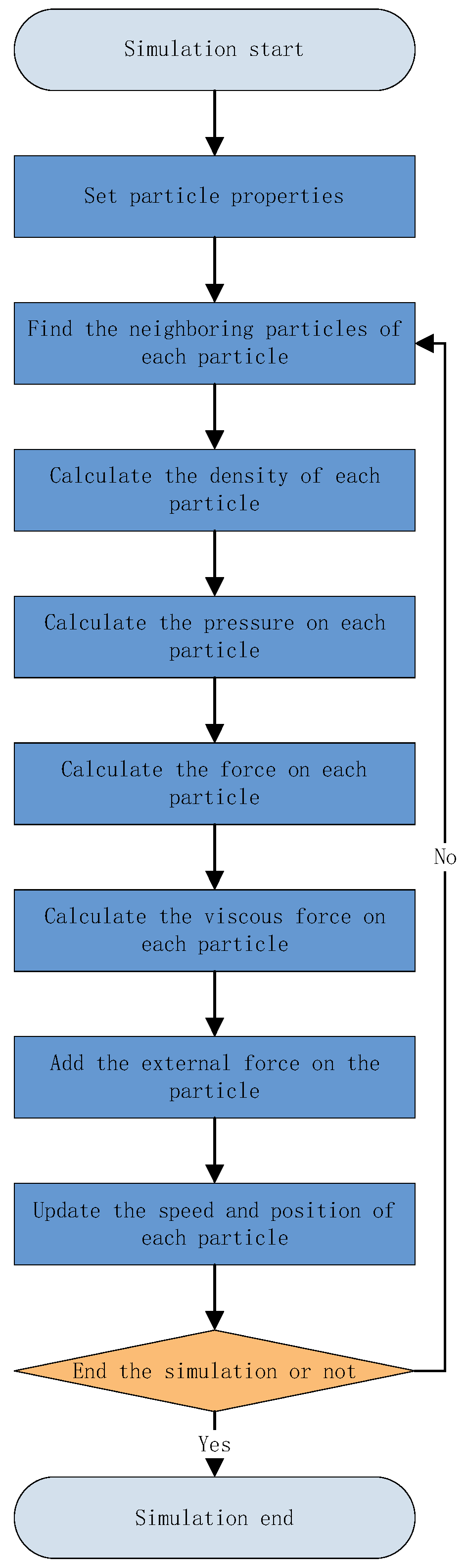
2.3. A Case Study of SPH

The formulation of smoothed particle hydrodynamics (SPH) equations is derived from the Navier–Stokes (N-S) equations. In the context of generalized fluid mechanics, both kernel and particle approximation methods are employed to spatially discretize these equations. This results in the development of SPH equations that are applicable to a broad range of fluid mechanics scenarios. The process yields a set of time-dependent ordinary differential equations that can be solved using time integration techniques. Consequently, the application of the SPH approximation method facilitates the spatial discretization of the Navier–Stokes equations, leading to the following representation of the SPH equation.
(1)
Mass conservation:
Density method:
ρ i = j = 1 N m j W i j
ρ i = j = 1 N m j W i j j = 1 N m j ρ j W i j
Continuity density method:
d ρ i d t = ρ i j = 1 N m j ρ j v i β v j β W i j x i β
d ρ i d t = j = 1 N m j v i β v j β W i j x i β
(2)
Momentum conservation:
d v i α d t = j = 1 N m j σ i α β ρ i 2 + σ j α β ρ j 2 W i j i β
(3)
Energy conservation:
d e i d t = 1 2 j = 1 N m j p i + p j ρ i ρ j v i j β W i j x i β + u i 2 ρ i ε i α β ε j α β
d e i d t = 1 2 j = 1 N m j p i ρ i 2 + p j ρ j 2 v i j β W i j x i β + u i 2 ρ i ε i α β ε j α β
The simulation steps of smoothed particle hydrodynamics (SPH) are depicted in Figure 6. Initially, fundamental properties such as position, velocity, mass, and other relevant parameters are assigned to each particle. Subsequently, neighboring particles are identified for each particle, with neighbors determined based on a specified distance using the kernel function. The density of each particle is then calculated by considering the mass and position of its neighboring particles, typically achieved through the accumulation of their contributions via the kernel function. Using the equation of state, the pressure for each particle is derived from the computed density. The pressure gradient is then employed to calculate the forces between particles, ensuring the effective simulation of fluid dynamic interactions. Additionally, to account for fluid viscosity, the internal friction effects are captured by evaluating the additional forces introduced by the gradient of the velocity. After calculating the internal forces, an external force, such as gravity, is applied to update the total force acting on each particle. Based on this total force, a time integration method is employed to update the velocity and position of the particles, ensuring that the simulation evolves accurately over time. Finally, upon completing a round of calculations, a decision is made regarding whether to continue the simulation. Depending on the established conditions, it is determined whether to conclude the simulation or return to the neighbor identification stage for the next round of calculations.
Through this series of steps, the SPH method effectively simulates the dynamic behavior of fluids. The simulation algorithm is outlined in Algorithm 1. In this context,
W represents the kernel function used for the smooth calculation of distances between particles;
H denotes the smoothing length, which determines the influence range of the kernel function;
Grad W refers to the gradient of the kernel function, utilized for force calculations;
Equation_of_state pertains to the state equation, which is employed to convert density into pressure;
Viscosity_term is a term that accounts for viscosity and is used to calculate the viscous force.
Algorithm 1: Smoothed particle hydrodynamics simulation algorithm
// Initialize particles
1:  for each particle i in fluid
2:    initialize_position(particle i)
3:    initialize_velocity(particle i)
4:    initialize_mass(particle i)
5:    initialize_other_properties(particle i)
6:  end for
// Main simulation loop
7:  while time < end_time
8:    // Compute density for each particle
9:    for each particle i in fluid
10:     rho_i = 0
11:     for each neighbor j of particle i
12:      rho_i += mass(j) * W(position(i) − position(j), H)
13:     end for
14:     density(i) = rho_i
15:    end for
16:    // Compute pressure for each particle
17:    for each particle i in fluid
18:     pressure(i) = equation_of_state(density(i))
19:    end for
20:    // Compute forces for each particle
21:    for each particle i in fluid
22:     force_i = 0
23:     for each neighbor j of particle i
24:      force_i += -mass(i) * (pressure(i) + pressure(j))/(2 * density(j)) * gradW(position(i) − position(j), H)
25:      + viscosity_term
26:     end for
27:     force(i) = force_i
28:    end for
29:    // Integrate motion equations
30:    for each particle i in fluid
31:     velocity(i) += time_step * force(i)/density(i)
32:     position(i) += time_step * velocity(i)
33:    end for
34:    // Handle boundary conditions
35:    for each particle i in fluid
36:     if position(i) is outside boundary
37:      handle_boundary(position(i), velocity(i))
38:     end if
39:    end for
40:    // Advance time
41:    time += time_step
42:  end while

3. Applications of Smooth Particle Hydrodynamics in Tunnel and Underground Engineering

3.1. Water and Mud Inrush during Tunnel Construction

In tunnel engineering, understanding the progressive damage to rock caused by water inrush is crucial due to the significant effects on structural integrity, ground stability, and project costs. Water ingress exacerbates rock deterioration by elevating pore pressure and promoting the dissolution of rock materials, which can lead to structural weakening, disrupted stress distributions, and potential instability. Such damage presents serious safety hazards, as the gradual degradation of rock may precipitate sudden, catastrophic failures, posing risks to personnel and complicating emergency management. Moreover, the financial impact is considerable, with increased needs for reinforcement, repairs, and project delays driving up costs. A comprehensive understanding of these processes is vital for formulating effective mitigation strategies, enhancing safety, and optimizing the performance and cost-effectiveness of tunneling operations.
Xia et al. [37] effectively replicate the entire process of progressive rock damage and water inrush, with the simulation results demonstrating that the improved SPH method is applicable to a variety of surface and underground challenges involving fluid–solid interactions. The key simulation results include the surface profile and velocity field for both the water and the elastic plate, as presented in Figure 7. At 0.2 s, the collapsed water body impacts the elastic plate, causing it to bend at the top and subsequently altering the direction of the water flow. The flow then overtops the plate, strikes the right wall, and gradually comes to a standstill.

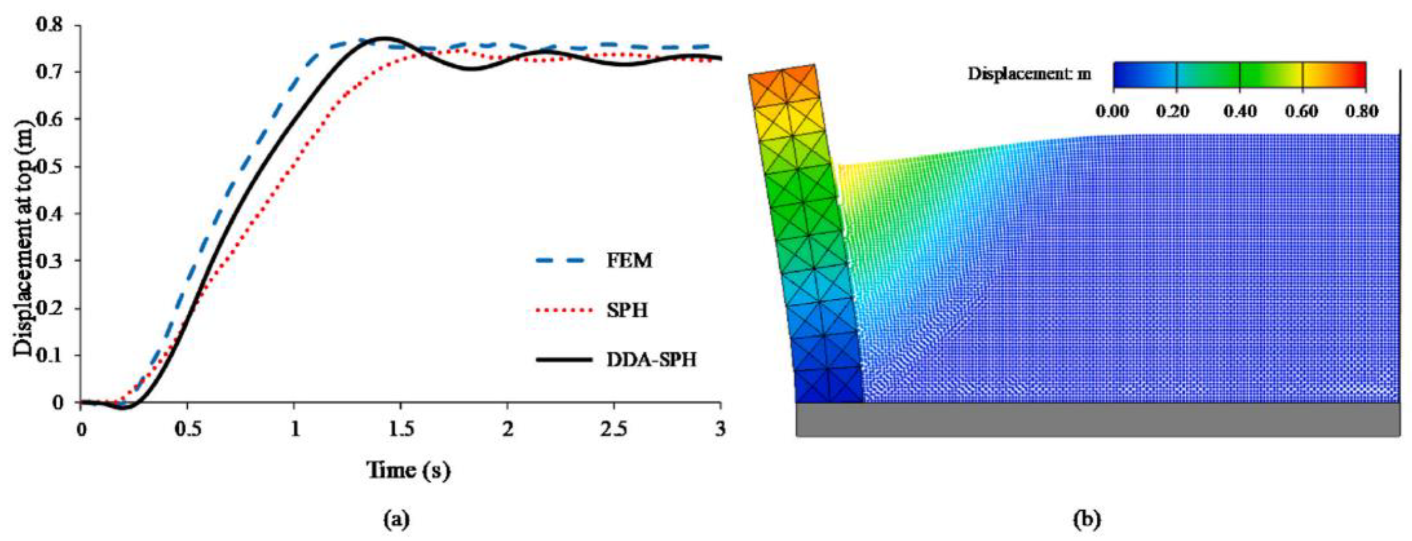
3.2. Interaction between Rock Structures and Soil

In tunnel engineering, the interactions between tunnel rock, soil, and retaining wall structures are crucial for ensuring structural stability, safety, and cost-effectiveness. This interaction affects key factors such as load distribution, ground response, and deformation characteristics. The precise modeling of these interactions is vital for anticipating and addressing potential challenges, which in turn supports the design of effective retaining walls and appropriate reinforcement measures. Additionally, a deep understanding of these dynamics aids in developing optimal design strategies, improving risk management, and ensuring the long-term performance and maintenance of the infrastructure. Therefore, a comprehensive grasp of these interactions is essential for the successful implementation and economic efficiency of tunneling projects.
Peng et al. [21] presented a simulation incorporating a novel spring-buffer contact model alongside the Mohr–Coulomb failure criterion. Upon verification, the results obtained from this approach exhibited enhanced accuracy, making it suitable for studying the impact of backfill on masonry arch bridges. Figure 8 presents the evolution of the horizontal displacement at the top of the retaining wall, along with the displacement profile at 3.0 s. The displacements calculated using the coupled DDA-SPH method are compared with those from other numerical methods, specifically the FEM and improved SPH62. The results show strong agreement in terms of deformation time history and maximum horizontal displacement. For instance, the maximum horizontal displacement is approximately 0.770 m, closely aligning with the 0.769 m predicted by the FEM and the 0.745 m predicted by improved SPH. This indicates that the coupled DDA-SPH method is effective for simulating interaction problems between granular soil and flexible structures.

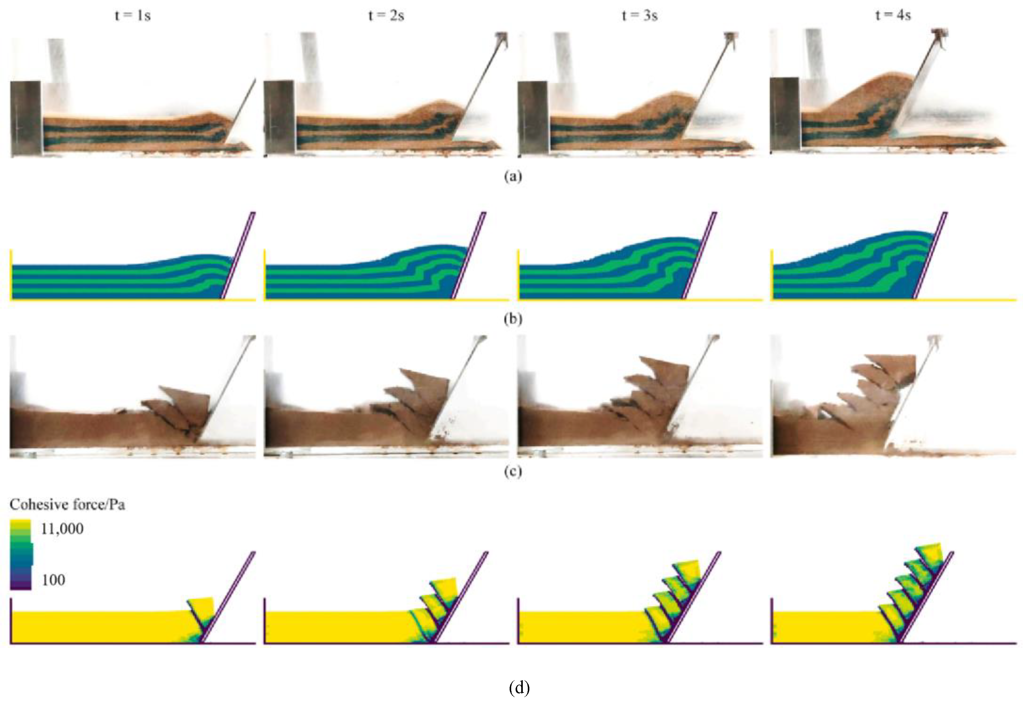
3.3. The Cutterhead Cuts Soil during Tunnel Construction

In relation to the process of tunnel construction, Hu et al. [22] simulated the cutting process and the interaction between the tool and both non-cohesive and cohesive soils using a shear failure model combined with a contact algorithm. The simulation results for non-cohesive and cohesive soils under various operating conditions were analyzed separately and then compared.
This paper provides a comparison between the SPH simulations and the experimental results for non-cohesive soils. As shown in Figure 9b, the simulation outcomes closely match the experimental results in Figure 9a. The numerical model, as depicted in Figure 9c, successfully replicates the process observed in the experiment. The number and shape of the small blocks chipped off by the blade align well with the experimental findings. Additionally, the model accurately represents the zigzag surface of the cracked cohesive soil mass and the detailed features at the tips of the chipped soil blocks. These results indicate that the model is effective in predicting the cutting behavior of cohesive soils. The model suggests that shear failures are most likely to occur in regions where plastic strains have accumulated over time. To mitigate tensile instability in all cohesive soil simulations, an artificial stress method was applied. One of the key advantages of numerical simulation is its ability to analyze microphysical quantities, such as stress and strain, which are challenging to measure experimentally.

4. Example Simulation and Analysis of SPH in Tunnel and Underground Engineering

While the SPH method is highly suitable for simulating the rheology of surrounding rock and the large deformations associated with tunnel construction, its application in this field faces significant limitations. Challenges arise due to the complex physical and mechanical properties of the surrounding rock, as well as the intricate constitutive models required for tunnel structures, particularly in terrains that are complex and irregular. The constraints include difficulties in representing complex terrain conditions, determining boundary conditions due to the challenges in defining the flow interface, and effectively addressing the boundary conditions in numerical methods. Additionally, accurately determining the source and quantity of fluid, such as sliding bodies or debris, and handling three-dimensional problems and multi-field coupling further complicate the use of SPH in these scenarios. Building on the above research, and supported by long-term on-site monitoring, a detailed simulation of blasting excavation for a mountain tunnel is provided below.

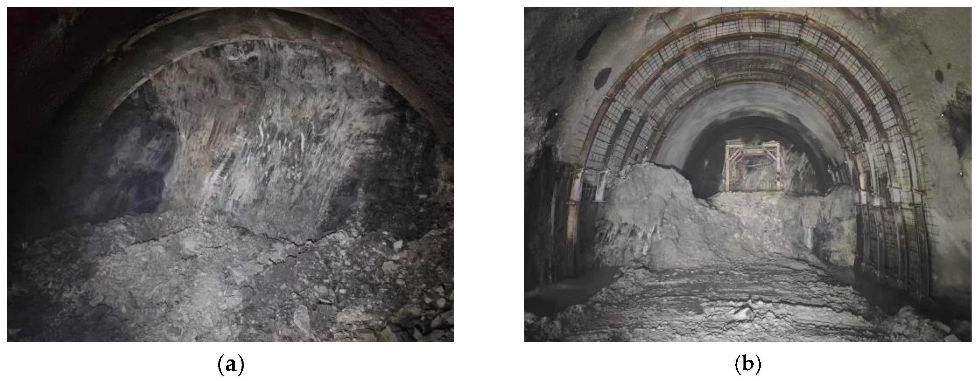
4.1. Engineering Background

The tunnel is situated adjacent to two other tunnels. The surface layer in this section consists of an artificial fill, varying in thickness from 1.1 to 8.6 m, underlain by a fully to weakly weathered granite layer classified as Grade V surrounding rock. Grade IV surrounding rock constitutes more than 80% of the entire tunnel. All three tunnels intersect the highway tunnel face simultaneously, as illustrated in the accompanying diagram. The tunnel’s stratigraphy predominantly comprises silty clay and granodiorite, with well-developed groundwater systems. Given the highly weathered nature of the surrounding rock and the close proximity of the other tunnels, stringent control over blasting-induced deformation and vibration is required. The tunnel palm support surface is shown in Figure 10.

4.2. Establishment of Numerical Simulation Model

This numerical simulation primarily investigates the extent of the damage to and the dynamic response of rock under blasting impact loads. For this study, the rock material was modeled using the material model *MAT_272, also known as *MAT_RHT, which effectively characterizes the damage range. The physical and mechanical parameters of the surrounding rock, based on field measurements, are presented in Table 1.
The high-energy explosive material model from the Ansys/LS-DYNA material library was selected to simulate the physical and chemical properties of explosives during the detonation process. The explosive is modeled as a uniform continuous medium using the keyword *MAT_HIGH_EXPLOSIVE_BURN. The material parameters were primarily referenced from the performance characteristics of granular viscous ammonium nitrate explosives provided by the mine. The specific explosive parameters are detailed in Table 2.
To mitigate boundary effects, the tunnel section is positioned at the center of the model, with the distance from the boundary set to four times the tunnel diameter. The surrounding rock is modeled using the SHELL163 shell element. The finite element mesh model is constructed with Ansys 19.0/LS-DYNA, employing the SPH method to simulate the explosives. Particle distribution within the model is managed using LS-PrePost 4.0 post-processing software. In the vertical stress field, a uniform load is applied to the top of the model to account for self-weight. The initial stress values in the horizontal stress field are adjusted according to the vertical gradient. A fixed constraint is applied at the bottom of the model, while force constraints are imposed on the upper boundary to simulate various working conditions at different burial depths. Additionally, force constraints are applied to the left and right boundaries to represent the varying lateral pressure coefficient. The model simulates the blasting excavation process, as depicted in Figure 11.

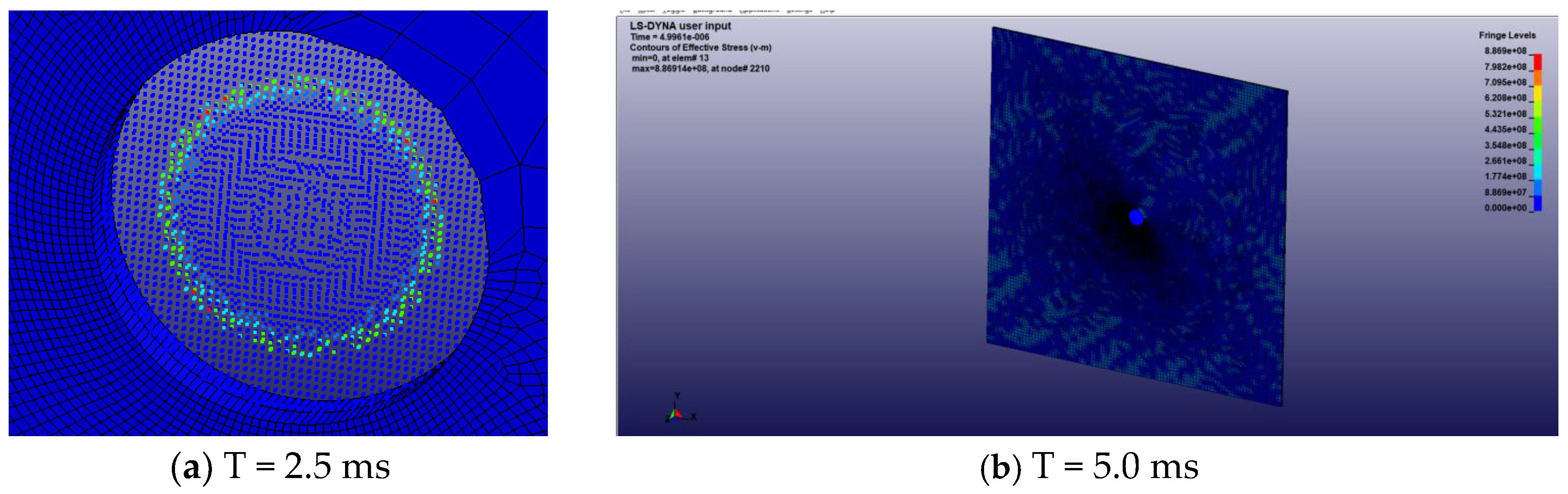
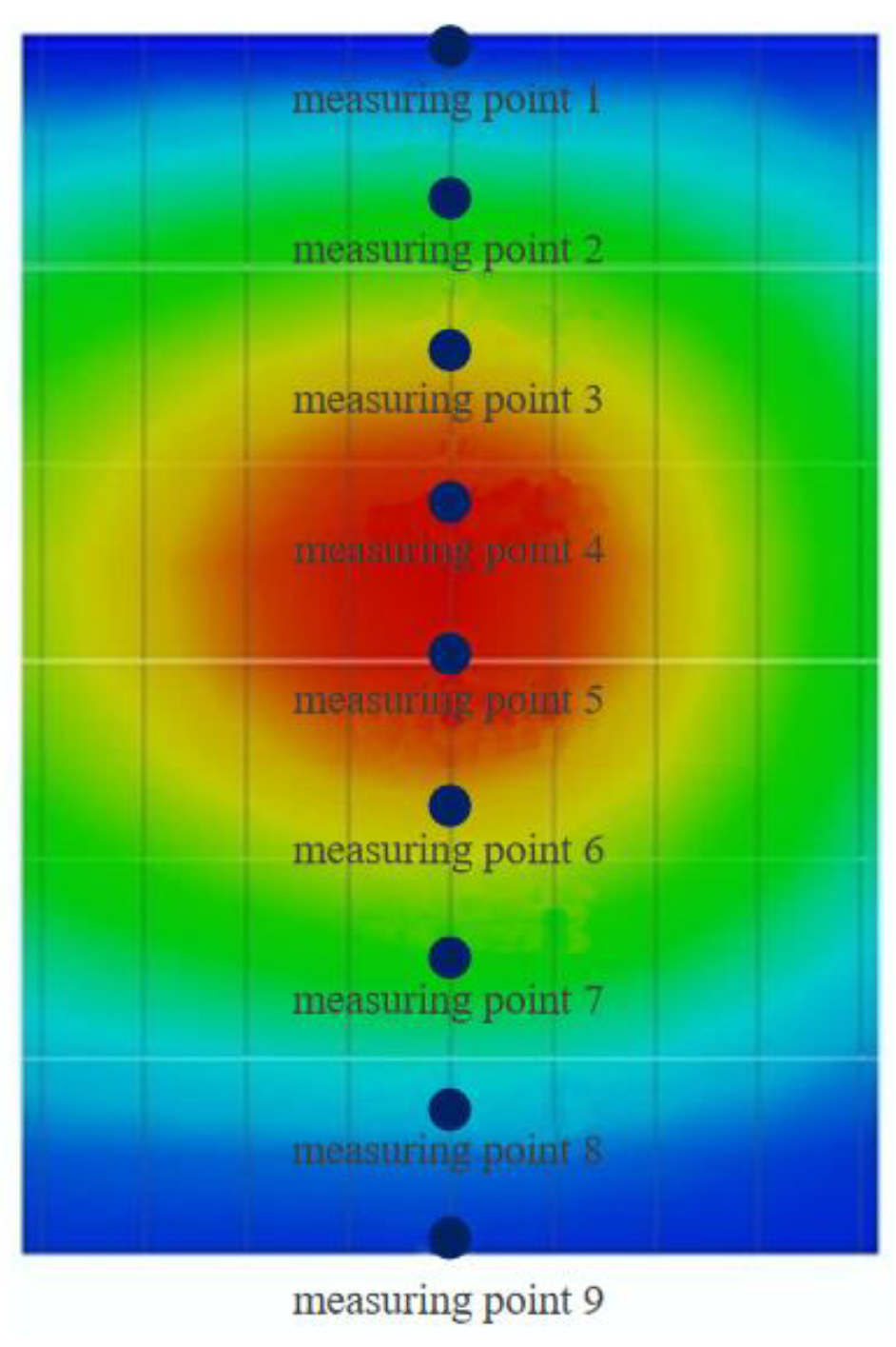
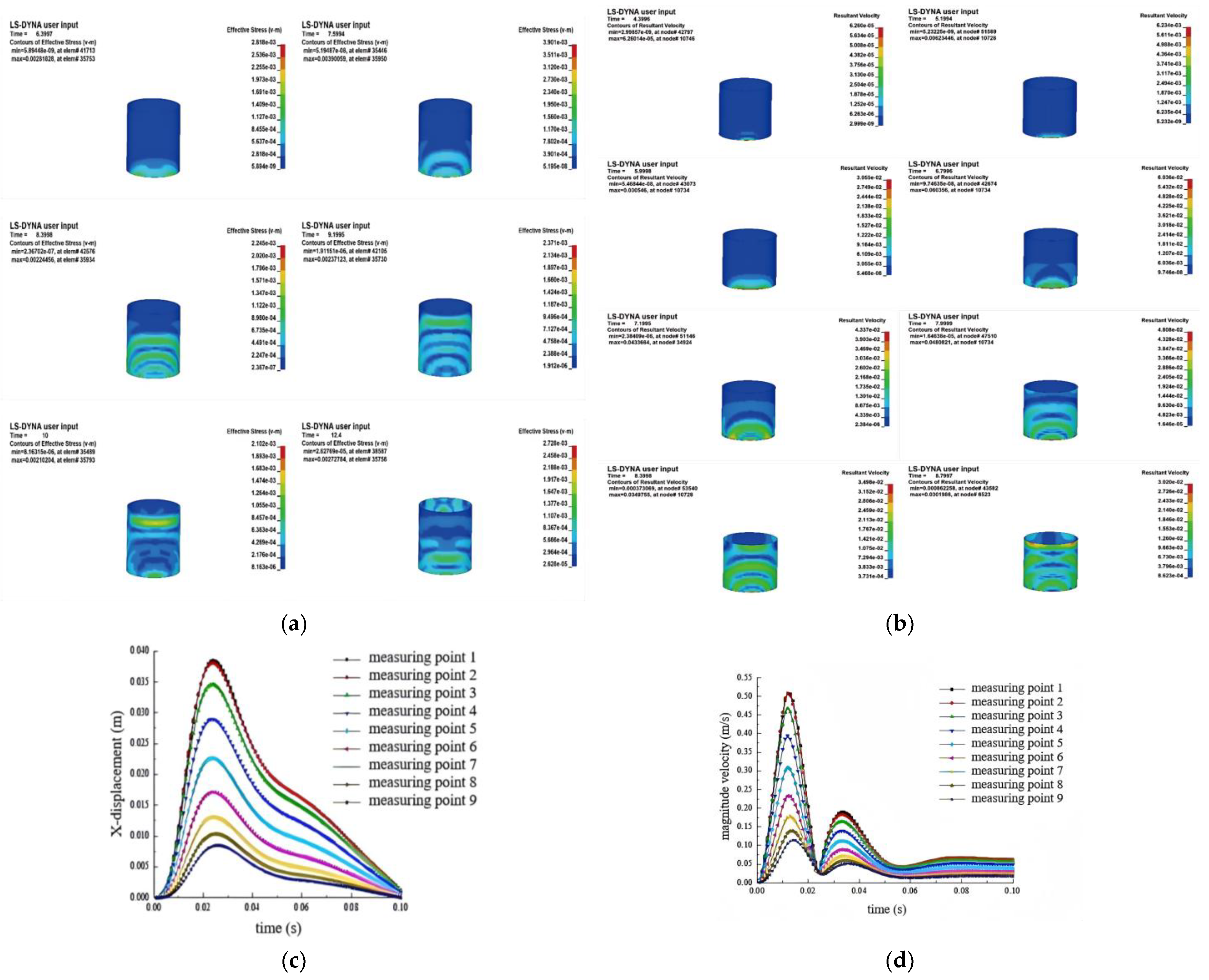
4.3. Numerical Simulation Results Analysis

The maximum displacement in the x-direction of the tunnel structure is concentrated in the central region of the blasting load, forming an approximately circular distribution. Due to the constraints at the upper and lower ends, the displacement exhibits an elliptical decay pattern, with faster attenuation in the vertical direction (up and down) and slower attenuation in the horizontal direction (left and right). The displacement and vibration velocities at the top measurement point are smaller than those observed at the bottom. To investigate the specific displacement and attenuation patterns at different advance distances, the results from the transverse and vertical measuring points in the tunnel’s center were extracted and compared (Figure 12). Additionally, these findings were cross-referenced with field monitoring data (Figure 13).
The model was extended into three dimensions, as depicted in Figure 14. From Figure 14a, it is observed that the tunnel structure adjacent to the tunnel face first experiences the blasting impact, occurring at approximately 4.3 ms. Over time, the blast-induced vibrations in the tunnel wall propagate radially from the inner center toward the periphery. During this phase, the vibration velocity distribution takes on an elliptical shape, with the affected area gradually expanding from the front side to the back side of the tunnel, reaching the inverted arch trestle at around 7.9 ms. The vibration velocity peaks during this process and subsequently begins to decay. The blast vibrations continue to propagate toward the rear side of the tunnel, ultimately affecting the entire tunnel structure by approximately 8.8 ms.
Figure 14b reveals that the effective stress initially increases and then decreases along the tunnel’s direction, with the maximum stress occurring at a distance of 2 m. This indicates that the region approximately 2 m from the blasting surface within the tunnel structure is a vulnerable area, prone to buckling. The highest circumferential effective stress at this location occurs at measuring point 1, situated at the center of the blasting side, which is the most susceptible to stress failure. Overall, the effective stress decreases initially and then shows a slight increase from the blasting surface along the circumference to the rear blasting surface.
Figure 14c illustrates that the displacement and vibration velocity at the top end of the tunnel are lower compared to those at the bottom. This discrepancy is attributed to the greater blasting load borne by the bottom section. The vibration velocity recorded at the transverse measuring point reveals two distinct vibration periods within the initial 50 ms, with the amplitude of the first period significantly exceeding that of the second. During this period, the first four columns of steel bars experience tensile forces, while the bars from the fifth column onwards are subjected to compression, with tensile forces surpassing compressive forces.
Figure 14d demonstrates that with a secondary lining thickness of 25 cm, the maximum vibration velocity reaches 49 cm/s, exceeding the allowable limit for safety. Increasing the thickness to 30 cm results in a reduction in the maximum vibration velocity to 32.6 cm/s, which conforms to the safety standard of 35 cm/s. Therefore, a secondary lining thickness of 30 cm is recommended for practical application. Although the stress on each component of the tunnel structure is maximized with a 25 cm thickness, all components remain within safe limits. Based on comprehensive analysis, the recommended thickness for the middle partition wall is 30 cm. These findings closely align with field measurement data and offer valuable theoretical guidance.

5. Conclusions

This paper explores the application of smoothed particle hydrodynamics (SPH) in tunnel and underground engineering, highlighting its capability to address complex issues related to large deformations and dynamic loading conditions. By deriving the theoretical framework of SPH and presenting two practical examples, this study validates the method’s efficacy in simulating intricate tunnel scenarios. SPH has emerged as a significant advancement in numerical simulation, offering a robust framework for analyzing and optimizing tunnel design and construction processes, as well as effectively managing large-scale deformations and dynamic loads. The findings from this research not only affirm SPH’s practical utility, but also establish a foundation for future advancements and refinements in numerical simulation techniques for tunnel and underground engineering. The key conclusions are summarized as follows:
(1)
This study provides a comprehensive examination of the application and future prospects of smoothed particle hydrodynamics (SPH) in tunnel and underground engineering. It thoroughly reviews the defining characteristics and theoretical foundations of the SPH method, supplemented with examples derived from the Navier–Stokes (N-S) equations. The discussion highlights SPH’s distinctive advantages in addressing complex flow dynamics and large deformation challenges. As a meshless technique, SPH demonstrates significant efficiency in managing dynamic boundaries, fluid–solid interactions, and multi-field coupling conditions.
(2)
As a meshless technique, smoothed particle hydrodynamics (SPH) offers distinct advantages for simulating fluid–solid interactions and multi-field coupling conditions, particularly in the dynamic environments of tunnel construction involving water and mud flows. SPH has demonstrated its versatility across a range of fields, including astrophysics, fluid dynamics, and solid mechanics. Its effectiveness in addressing various physical phenomena and incorporating material properties underscores its ability to enhance the accuracy of simulation results. The applicability of SPH is further validated through simulations of water and mud behavior during tunnel construction, the interaction between rock and soil structures, and the failure mechanisms of brittle materials.
(3)
This paper provides an in-depth examination of the theoretical foundations of smoothed particle hydrodynamics (SPH) and its potential applications in tunnel excavation and underground engineering. SPH has proven effective in simulating fluid dynamics and soil deformation during tunnel blasting, with simulation outcomes aligning closely with actual monitoring data. This validates the method’s feasibility and effectiveness for practical engineering applications. Despite its notable performance in managing large deformations in soft rocks and the mechanical cutting of hard rocks, SPH faces significant challenges. These include the complexity of constitutive models for surrounding rock masses, the rheological characteristics of tunnel structures, and the inherent spatiotemporal effects during excavation. Additionally, the fundamental theory of SPH requires further development, particularly in multi-field coupling scenarios. As computational resources and SPH theory continue to advance, the method’s applicability in tunnel and underground engineering is expected to expand. Future research should focus on addressing current technological limitations and exploring synergistic approaches with other numerical simulation techniques to enhance SPH’s utility in complex engineering environments. In summary, SPH, as an emerging numerical simulation tool, holds significant promise for tunnel and underground engineering and warrants further investigation and practical application.

Author Contributions

Conceptualization, R.F. and T.C.; methodology, R.F.; software, T.C.; validation, M.L. and S.W.; formal analysis, R.F.; investigation, R.F.; resources, T.C.; data curation, M.L.; writing—original draft preparation, R.F.; writing—review and editing, T.C.; visualization, S.W.; supervision, T.C.; project administration, R.F. All authors have read and agreed to the published version of the manuscript.

Funding

This research received no external funding.

Institutional Review Board Statement

Not applicable.

Informed Consent Statement

Not applicable.

Data Availability Statement

The original contributions presented in the study are included in the article, further inquiries can be directed to the corresponding author.

Conflicts of Interest

The authors declare no conflict of interest.

References

  1. Monaghan, J. An introduction to SPH. Comput. Phys. Commun. 1988, 48, 89–96. [Google Scholar] [CrossRef]
  2. Sun, X.; Wang, J. The theory and application of SPH method. Water Resour. Hydropower Technique 2007, 38, 44–46. [Google Scholar] [CrossRef]
  3. Tang, Y.; Shi, F.; Liao, X.; Zhou, S. Discussion on the influence of flow rule based on smooth particle hydrodynamics on large deformation of soil landslide. Rock. Soil. Mechan. 2018, 39, 1509–1516. [Google Scholar] [CrossRef]
  4. Yan, J.; Cheng, Y. Deep Learning-Meshless Method for Inverse Potential Problems. Int. J. Appl. Mech. 2024, 16, 2450069. [Google Scholar] [CrossRef]
  5. Liu, M.B.; Liu, G.R.; Zong, Z. An overview on smoothed particle hydrodynamics. Int. J. Comput. Methods 2008, 5, 135–188. [Google Scholar] [CrossRef]
  6. Yang, X.-F.; Liu, M.-B. An improved scheme for stress instability of smoothed particle dynamics SPH method. Acta Phys. Sin. 2012, 61, 224701. [Google Scholar] [CrossRef]
  7. Antoci, C.; Gallati, M.; Sibilla, S. Numerical simulation of fluid–structure interaction by SPH. Comput. Struct. 2007, 85, 879–890. [Google Scholar] [CrossRef]
  8. Yu, H.; Liang, H.; Hideto, N. The state of the art of SPH method applied in geotechnical engineering. Chin. J. Geotech. Eng. 2008, 30, 256–262. [Google Scholar] [CrossRef]
  9. Wijesooriya, K.; Mohotti, D.; Lee, C.-K.; Mendis, P. A technical review of computational fluid dynamics (CFD) applications on wind design of tall buildings and structures: Past, present and future. J. Build. Eng. 2023, 74, 106828. [Google Scholar] [CrossRef]
  10. Tu, X.L.; Gambaruto, A.M.; Newell, R.; Pregnolato, M.; Tu, X.L.; Gambaruto, A.M.; Newell, R.; Pregnolato, M. Computational fluid dynamics analysis of bridge scour with a comparison of pier shapes and a debris fin. Structures 2024, 67, 106966. [Google Scholar] [CrossRef]
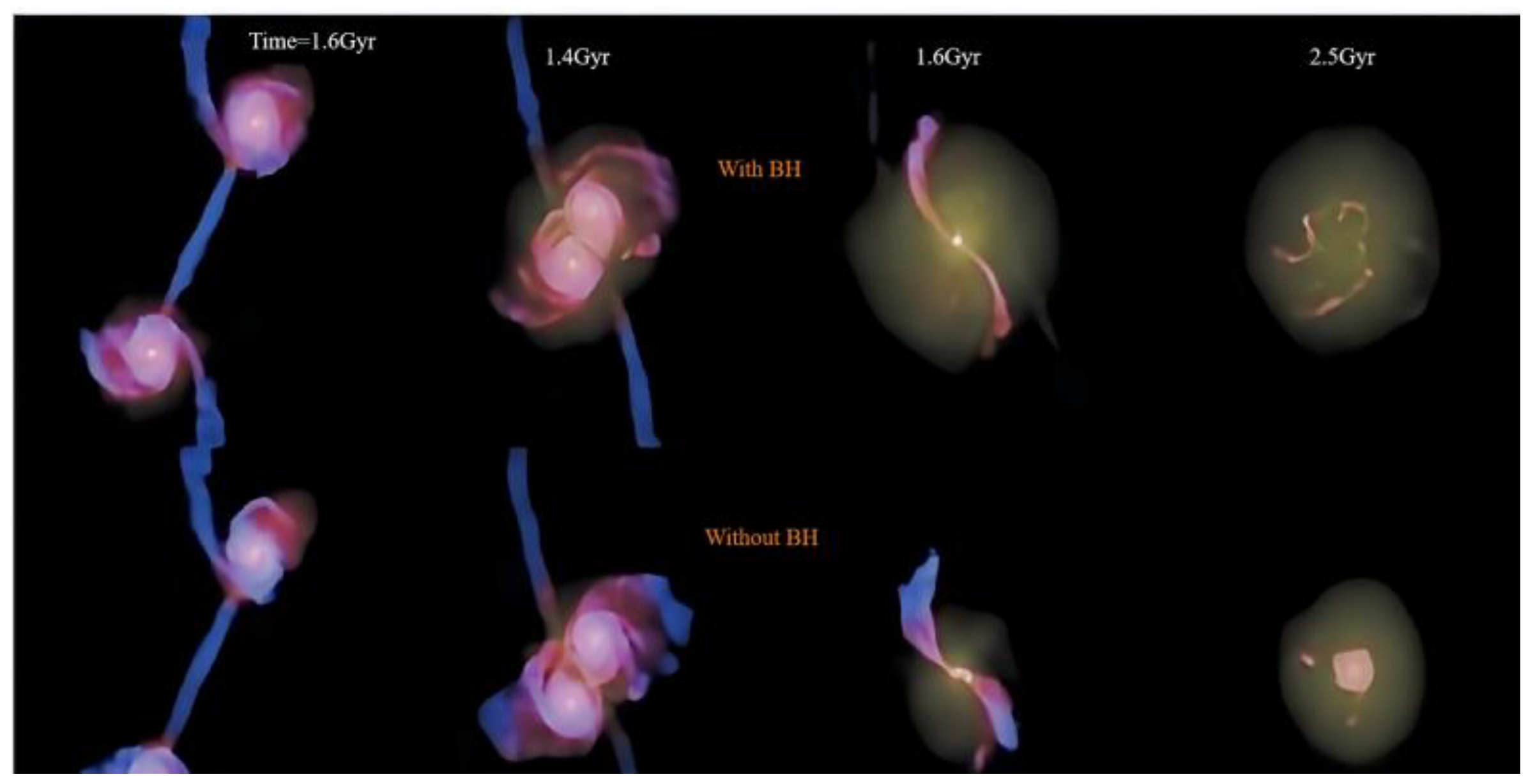
  11. Mirza, M.A.; Tahir, A.; Khan, F.M.; Holley-Bockelmann, H.; Baig, A.M.; Berczik, P.; Chishtie, F. Galaxy rotation and supermassive black hole binary evolution. Mon. Not. R. Astron. Soc. 2017, 470, 940–947. [Google Scholar] [CrossRef]
  12. Kazemi, E.; Koll, K.; Tait, S.; Shao, S. SPH modelling of turbulent open channel flow over and within natural gravel beds with rough interfacial boundaries. Adv. Water Resour. 2020, 140, 103557. [Google Scholar] [CrossRef]
  13. Meringolo, D.D.; Marrone, S.; Colagrossi, A.; Liu, Y. A dynamic δ-SPH model: How to get rid of diffusive parameter tuning. Comput. Fluids 2019, 179, 334–355. [Google Scholar] [CrossRef]
  14. Wu, J.-H.; Chen, C.-H. Application of DDA to simulate characteristics of the Tsaoling landslide. Comput. Geotech. 2011, 38, 741–750. [Google Scholar] [CrossRef]
  15. Xiang, Z.; Yu, S.; Wang, X. Modeling the Hydraulic Fracturing Processes in Shale Formations Using a Meshless Method. Water 2024, 16, 1855. [Google Scholar] [CrossRef]
  16. Xiong, W.; Cai, C.; Kong, B.; Kong, X. CFD simulations and analyses for bridgescour development using a dynamic-mesh updating technique. J. Comput. Civ. Eng. 2016, 30, 04014121. [Google Scholar] [CrossRef]
  17. Zhang, J.; Wang, B.; Hou, G. Numerical simulation and experimental study of fluid–structure interactions in elastic structures based on the SPH method. Ocean. Eng. 2024, 301, 117523. [Google Scholar] [CrossRef]
  18. Bo, X.; Mowen, X.; Man, H. Research on SPH particle model of landslide based on GIS spatial data. Rock. Soil. Mech. 2016, 37, 2696–2705. [Google Scholar] [CrossRef]
  19. Pan, J.; Zeng, Q. Research review over the advances of the application of SPH method to the analysis of the serious geotechnical deformation. J. Saf. Environ. 2015, 15, 144–150. [Google Scholar] [CrossRef]
  20. Lian, Y.; Bui, H.H.; Nguyen, G.D.; Haque, A. An effective and stabilised (u−pl) SPH framework for large deformation and failure analysis of saturated porous media. Comput. Methods Appl. Mech. Eng. 2023, 408, 115967. [Google Scholar] [CrossRef]
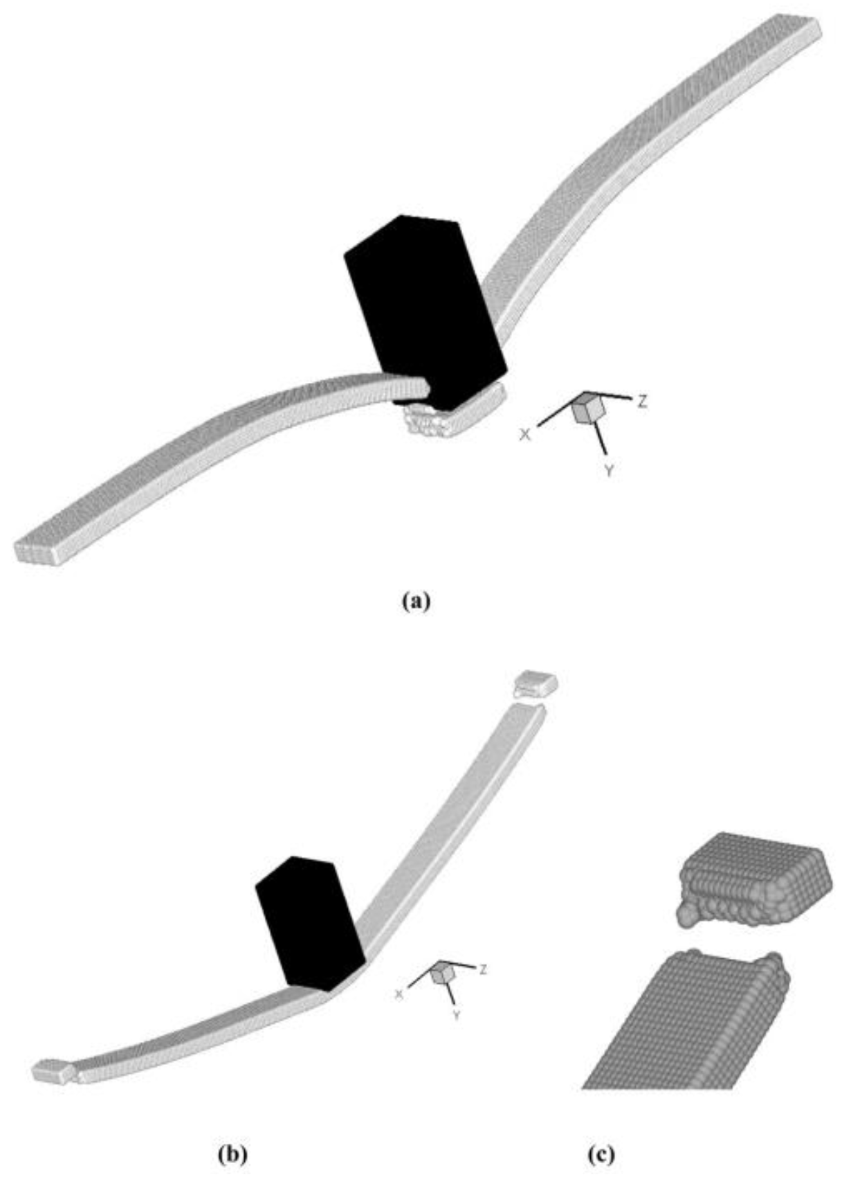
  21. Peng, X.; Chen, G.; Fu, H.; Yu, P.; Zhang, Y.; Tang, Z.; Zheng, L.; Wang, W. Development of coupled DDA-SPH method for dynamic modelling of interaction problems between rock structure and soil. Int. J. Rock. Mech. Min. Sci. Géoméch. Abstr. 2021, 146, 104890. [Google Scholar] [CrossRef]
  22. Hu, M.; Gao, T.; Dong, X.; Tan, Q.; Yi, C.; Wu, F.; Bao, A. Simulation of soil-tool interaction using smoothed particle hydrodynamics (SPH). Soil. Tillage Res. 2023, 229, 105671. [Google Scholar] [CrossRef]
  23. Chakraborty, S.; Shaw, A. A pseudo-spring based fracture model for SPH simulation of impact dynamics. Int. J. Impact Eng. 2013, 58, 84–95. [Google Scholar] [CrossRef]
  24. Lu, G.; Tao, C.; Xia, C.; Cao, B.; Zhu, X. Stability analysis of layered circular rock tunnels considering anchor reinforcement based on an enhanced mesh-free method. Eng. Anal. Bound. Elem. 2024, 166, 105850. [Google Scholar] [CrossRef]
  25. Beyabanaki, S.A.R.; Bagtzoglou, A.C.; Liu, L. Applying disk-based discontinuous deformation analysis (DDA) to simulate Donghekou landslide triggered by the Wenchuan earthquake. Géoméch. Geoengin. 2016, 11, 177–188. [Google Scholar] [CrossRef]
  26. Lee, E.M. Landslide risk assessment: The challenge of communicating uncertainty to decision-makers. Q. J. Eng. Geol. Hydrogeol. 2016, 49, 21–35. [Google Scholar] [CrossRef]
  27. Sekine, H.; Ito, R.; Shintate, K. A single energy-based parameter to assess protection capability of debris shields. Int. J. Impact Eng. 2007, 34, 958–972. [Google Scholar] [CrossRef]
  28. Tang, Y.; Shi, F.; Liu, X. Failure criteria based on SPH slope stability analysis. Chin. J. Geotech. Eng. 2016, 38, 904–908. [Google Scholar] [CrossRef]
  29. He, F.; Chen, Y.; Wang, L.; Li, S.; Huang, C. A multi-layer SPH method to simulate water-soil coupling interaction-based on a new wall boundary model. Eng. Anal. Bound. Elem. 2024, 164, 105755. [Google Scholar] [CrossRef]
  30. Hu, M.; Liu, M.B.; Xie, M.W.; Liu, G.R. Three-dimensional run-out analysis and prediction of flow-like landslides using smoothed particle hydrodynamics. Environ. Earth Sci. 2015, 73, 1629–1640. [Google Scholar] [CrossRef]
  31. Cleary, P.; Ha, J.; Prakash, M.; Nguyen, T. 3D SPH flow predictions and validation for high pressure die casting of automotive components. Appl. Math. Model. 2006, 30, 1406–1427. [Google Scholar] [CrossRef]
  32. Morris, J.P.; Fox, P.J.; Zhu, Y. Modeling Low Reynolds Number Incompressible Flows Using SPH. J. Comput. Phys. 1997, 136, 214–226. [Google Scholar] [CrossRef]
  33. Bui, H.H.; Fukagawa, R.; Sako, K.; Ohno, S. Lagrangian meshfree particles method (SPH) for large deformation and failure flows of geomaterial using elastic–plastic soil constitutive model. Int. J. Numer. Anal. Methods Géoméch. 2008, 32, 1537–1570. [Google Scholar] [CrossRef]
  34. Nonoyama, H.; Moriguchi, S.; Sawada, K.; Yashima, A. Slope stability analysis using smoothed particle hydrodynamics (SPH) method. Soils Found. 2015, 55, 458–470. [Google Scholar] [CrossRef]
  35. Chen, J.K.; Beraun, J.E.; Carney, T.C. A corrective smoothed particle method for boundary value problems in heat conduction. Int. J. Numer. Methods Eng. 1999, 46, 231–252. [Google Scholar] [CrossRef]
  36. Xia, C.; Shi, Z.; Li, B. a modified SPH framework of for simulating progressive rock damage and water inrush disasters in tunnel constructions. Comput. Geotech. 2024, 167, 106042. [Google Scholar] [CrossRef]
  37. Bao, Y.; Ye, G.; Ye, B.; Zhang, F. Seismic evaluation of soil–foundation–superstructure system considering geometry and material nonlinearities of both soils and structures. Soils Found. 2012, 52, 257–278. [Google Scholar] [CrossRef]
  38. Nonoyama, H. Application of SPH method in geotechnical engineering. J. Sand Control. Soc. 2015, 68, 68–71. [Google Scholar] [CrossRef]
  39. Man, H.; Fei, W.; Shiji, W.; Fuyu, Z. Modeling of influenced area after slope failure based on smoothed particle hydrodynamics (SPH). J. Chongqing Univ. 2019, 42, 56–65. [Google Scholar] [CrossRef]
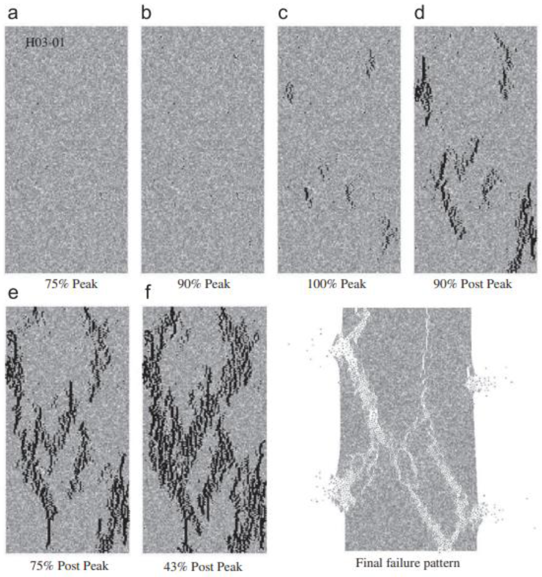
  40. Ma, G.; Wang, X.; Ren, F. Numerical simulation of compressive failure of heterogeneous rock-like materials using SPH method. Int. J. Rock. Mech. Min. Sci. Géoméch. Abstr. 2011, 48, 353–363. [Google Scholar] [CrossRef]
Figure 1. Planetary composition process diagram.
Applsci 14 08552 g001
Figure 2. Deformed configuration with (a) initial velocity of 60 m/s and (b) initial velocity of 40 m/s; (c) enlarged view at fracture point.
Applsci 14 08552 g002
Figure 3. Seepage process simulation diagram.
Applsci 14 08552 g003
Figure 4. Predicted failure process and final failure pattern for specimen H03-01. (a) One can observe the isolated microcracks are randomly distributed throughout the specimen (b) The density of microcracks increases but the specimen still maintainsintegrity and stability. (c) A few clusters of the microcracks form isolated fractures or cracks. (d) These isolated fractures grow rapidly At stage (e,f), more fractures coalesce and interact with each other and further develop into inclined shear faults across the specimen.
Applsci 14 08552 g004
Figure 5. Stabilised SPH prediction of the pore water pressure induced by contraction in the retrogressive failure of sensitive clay slope with K0 = 0.5.
Applsci 14 08552 g005
Figure 6. The simulation steps of the SPH method.
Applsci 14 08552 g006
Figure 7. Results of surface profile and velocity field for water and elastic plate using the SPH method.
Applsci 14 08552 g007
Figure 8. Deformation of the retaining wall system: (a) the evolution of the horizontal displacement at the top of the retaining wall, and (b) the displacement profile at 3.0 s.
Applsci 14 08552 g008
Figure 9. Simulation and experimental results of the cutting process for non-cohesive soil and cohesive soil: (a) the configuration of the cutting experiment for non-cohesive soil; (b) the configuration of cutting simulations for non-cohesive soil; (c) the configuration of the cutting experiment for cohesive soil; (d) the configuration of cutting simulations of cohesive soil.
Applsci 14 08552 g009
Figure 10. The process of tunnel face excavation by the blasting method. (a) Tunnel face disclosure; (b) Tunnel support schematic diagram.
Applsci 14 08552 g010
Figure 11. Numerical simulation of blasting excavation process.
Applsci 14 08552 g011
Figure 12. Monitoring point layout diagram.
Applsci 14 08552 g012
Figure 13. Field monitoring diagram.
Applsci 14 08552 g013
Figure 14. (a) Effective stress cloud diagram of tunnel structure. (b) Vibration velocity response of tunnel wall. (c) Displacement of tunnel and surrounding rock. (d) Combined velocity of tunnel and surrounding rock.
Applsci 14 08552 g014
Table 1. Physical and mechanical parameter values of surrounding rock.
Surrounding Rock ClassificationVolumetric Weight/(kN/m3)E/(GPa)Poisson RatioAngle of Internal Friction/(°)Cohesion/(MPa)
Va191.650.37240.16
Table 2. Physical and mechanical parameter values of high-energy explosive material.
Density/(g·cm−3)Detonation Velocity/(m·s−1)C-J Pressure/(GPa)
0.9531504.0
Disclaimer/Publisher’s Note: The statements, opinions and data contained in all publications are solely those of the individual author(s) and contributor(s) and not of MDPI and/or the editor(s). MDPI and/or the editor(s) disclaim responsibility for any injury to people or property resulting from any ideas, methods, instructions or products referred to in the content.

