
Accessing Near-Field Strong Ground Motions Using a Multi-Scheme Method in the Kalawenguquan Fault, Xinjiang, China


Abstract
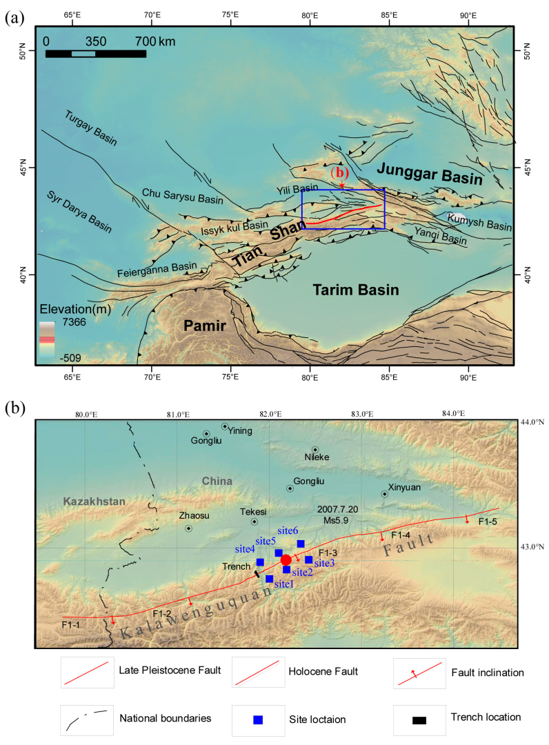
:1. Introduction
2. Materials and Methods
2.1. Materials
2.1.1. Maximum Credible Earthquake Magnitude
2.1.2. Dip Angle
2.1.3. Rupture Length and Width
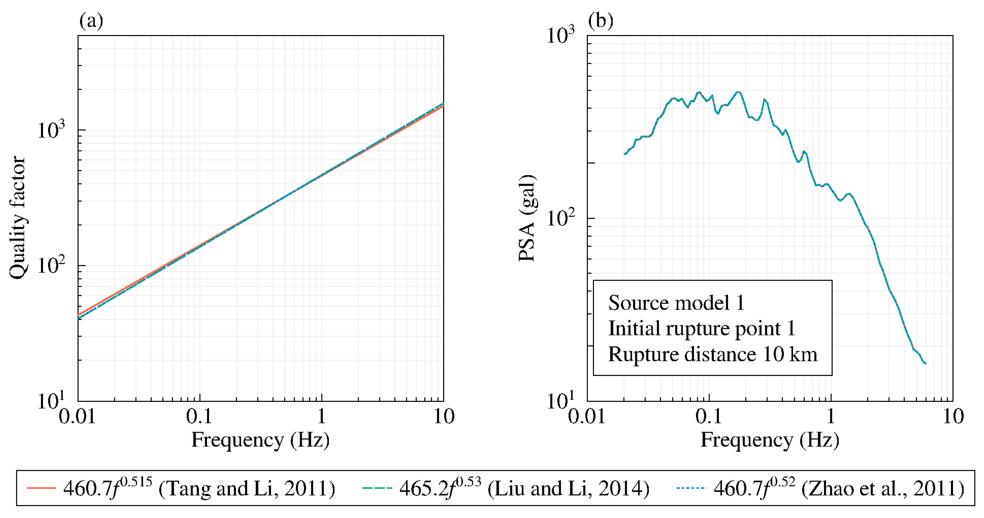
2.1.4. Quality Factor
2.1.5. Stress Drop
2.1.6. High-Frequency Attenuation
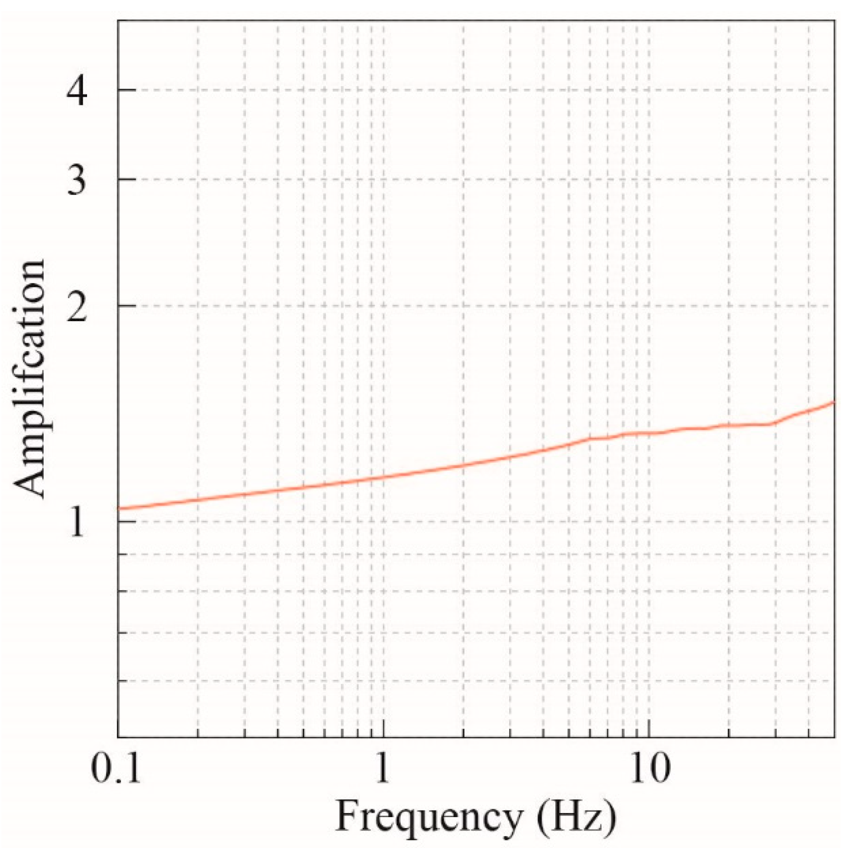
2.1.7. Site Amplification Factor
2.2. Source Model
2.2.1. Slip Model 1
2.2.2. Slip Model 2
2.3. Stochastic Finite-Fault Modeling Methods
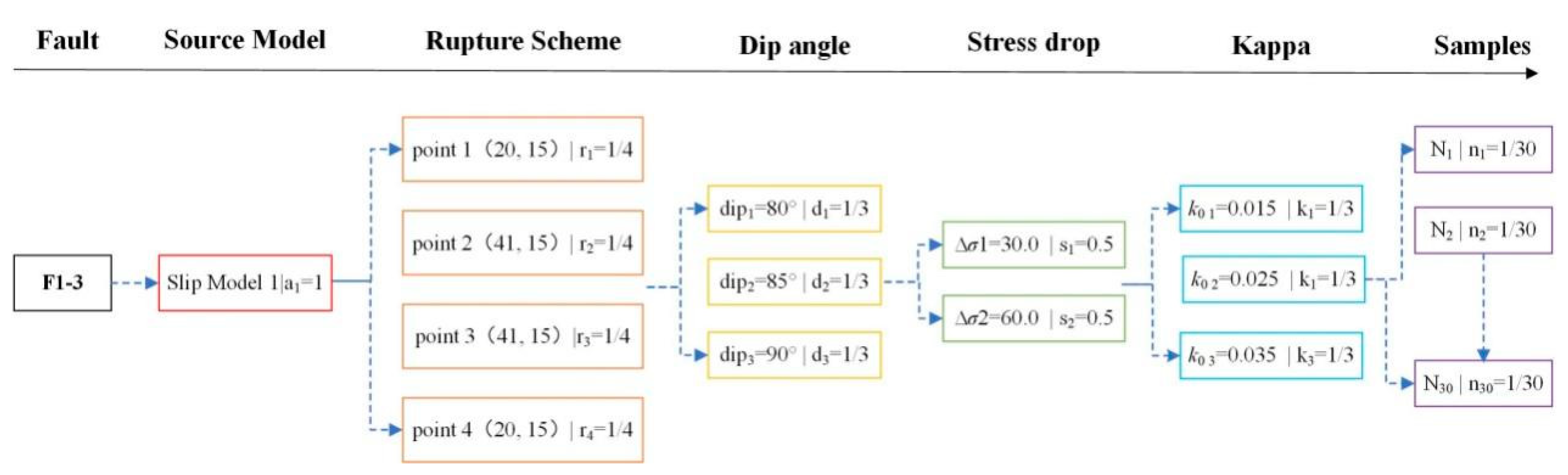
2.4. Multi-Scheme Ground Motion Simulations
3. Results
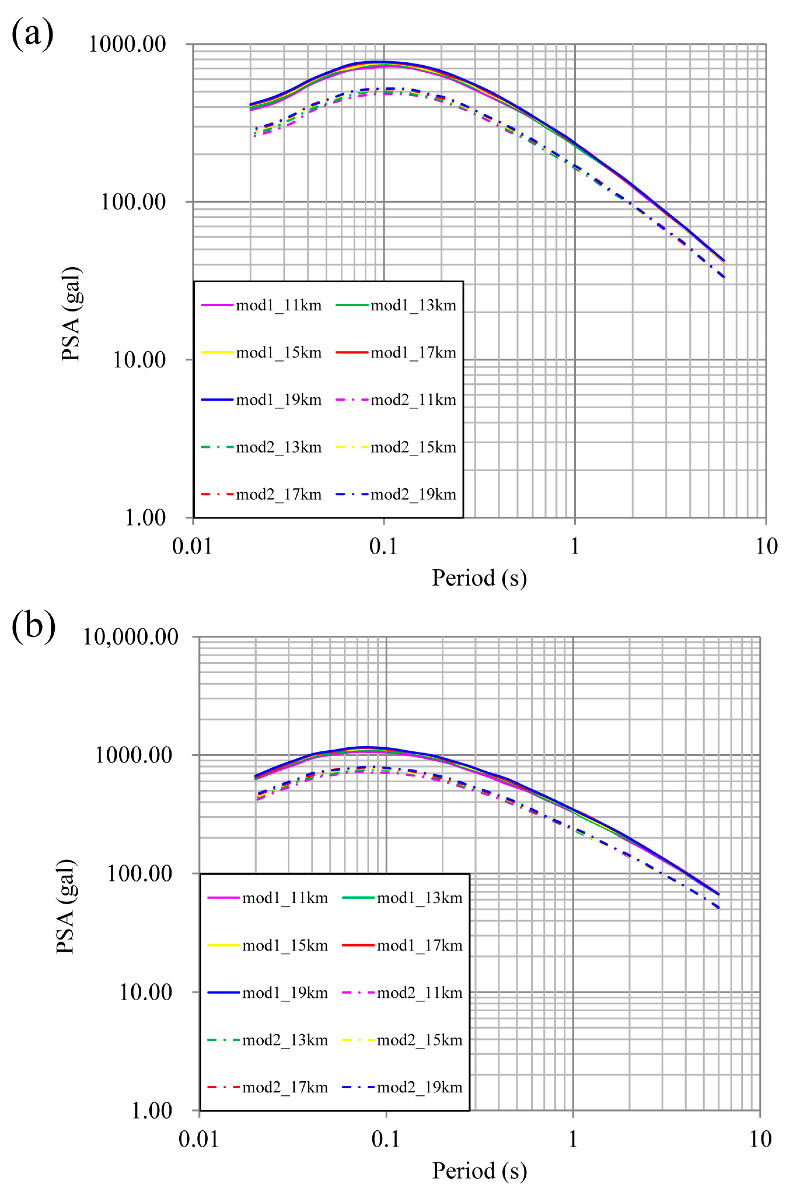
3.1. The Influence of Slip Models
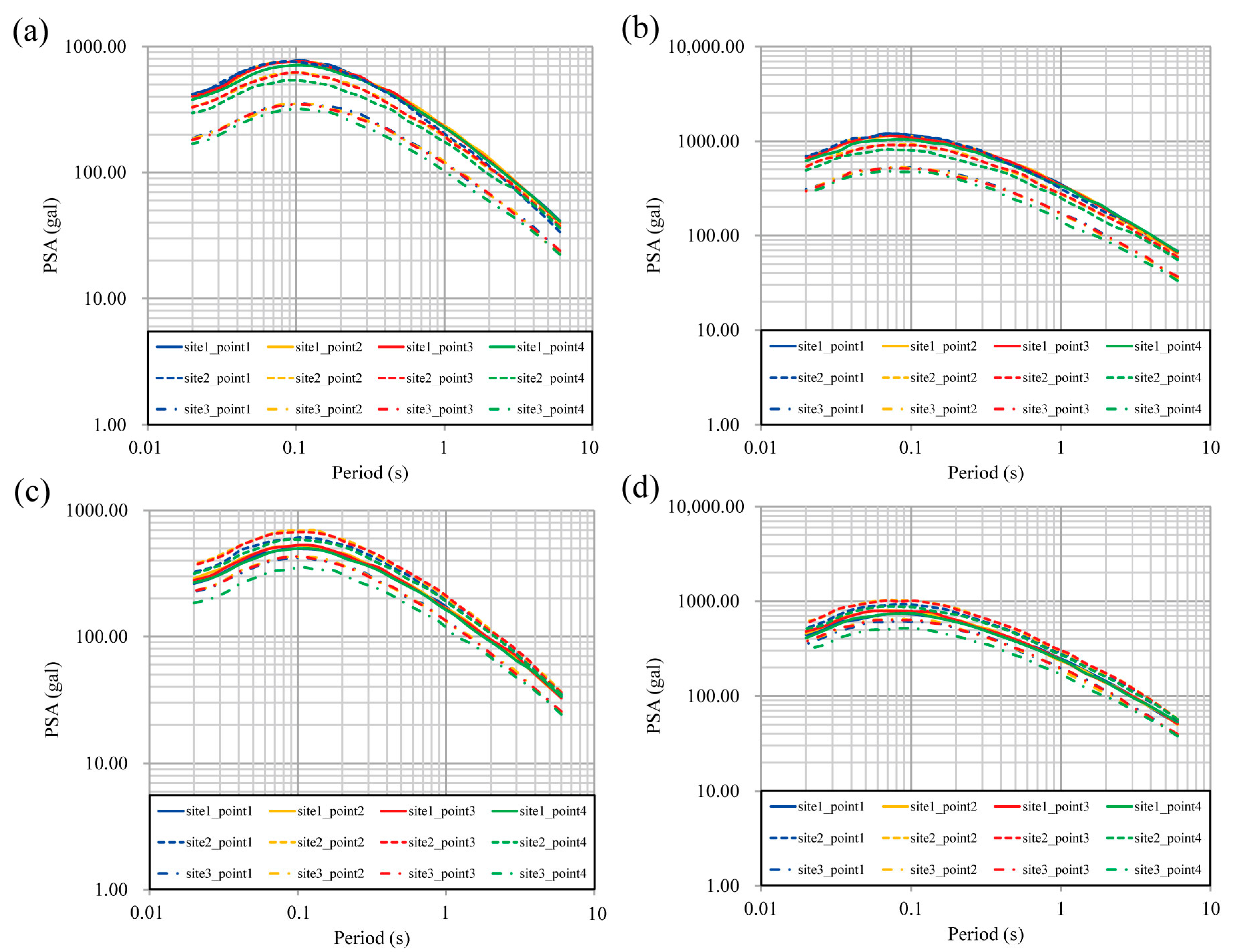
3.2. The Influence of Initial Rupture Points
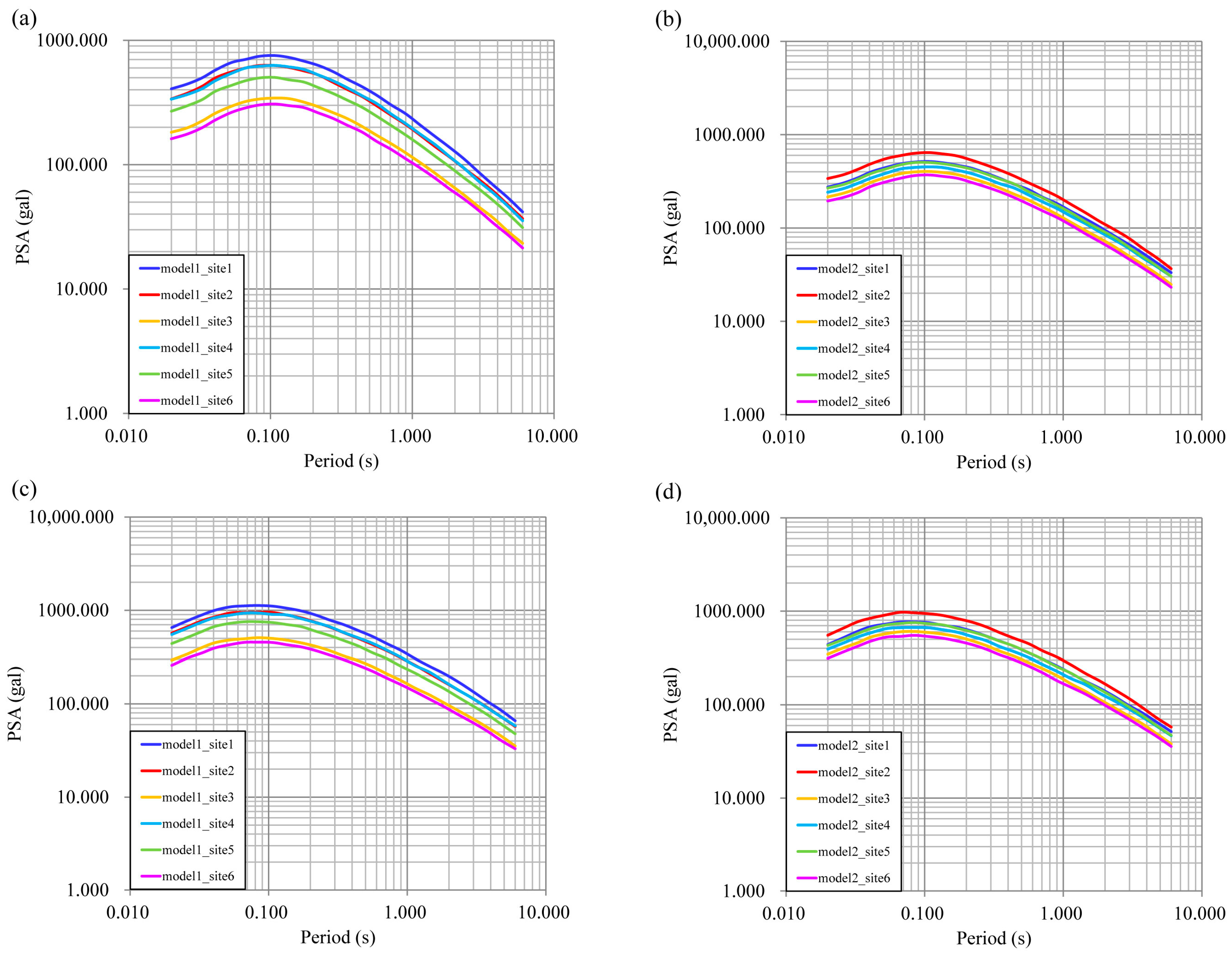
3.3. The Influence of Sites
4. Discussion and Conclusions
Supplementary Materials
Author Contributions
Funding
Institutional Review Board Statement
Informed Consent Statement
Data Availability Statement
Conflicts of Interest
References
- Kang, J.M.; Wang, Z.H.; Cheng, H.B.; Wang, J.; Liu, X.L. Remote sensing land use evolution in earthquake-stricken regions of Wenchuan county, China. Sustainability 2022, 14, 9721. [Google Scholar] [CrossRef]
- Shareef, S.S. Earthquake consideration in architectural design: Guidelines for architects. Sustainability 2023, 15, 13760. [Google Scholar] [CrossRef]
- EN 1998-1-2:2019.2; Design of Structures for Earthquake Resistance—Part 1: General Rules, Seismic Actions and Rules for Buildings. European Committee for Standardization: Brussels, Belgium, 2019.
- International Code Council (ICC). 2018 International Building Code; International Code Council (ICC): Nappanee, IN, USA, 2017. [Google Scholar]
- GB50011-2010; Code for Seismic Design of Buildings. China Building Industry Press: Beijing, China, 2010.
- American Society of Civil Engineers. Minimum Design Loads for Buildings and Other Structures; ASCE: Reston, VI, USA, 2010. [Google Scholar]
- Yu, Y.X.; Li, S.Y.; Xiao, L. Development of ground motion attenuation relations for the new seismic hazard map of China. Technol. Earthq. Disast. Prev. 2013, 8, 24–33. [Google Scholar]
- Abrahamson, N.A.; Silva, W.J.; Kamai, R. Summary of the ASK14 ground motion relation for active crustal regions. Earthq. Spectra 2014, 30, 1025–1055. [Google Scholar] [CrossRef]
- Boore, D.M.; Stewart, J.P.; Seyhan, E.; Atkinson, G.M. NGA-West2 equations for predicting PGA, PGV, and 5% damped PSA for shallow crustal earthquake. Earthq. Spectra 2014, 30, 1057–1085. [Google Scholar] [CrossRef]
- Campbell, K.W.; Bozorgnia, Y. Average horizontal components of PGA, PGV, and 5% damped linear acceleration response spectra. Earthq. Spectra 2014, 30, 1087–1115. [Google Scholar] [CrossRef]
- Chiou, B.S.J.; Youngs, R.R. Update of the Chiou and Youngs NGA model for the average horizontal component of peak ground motion and response spectra. Earthq. Spectra 2014, 30, 1117–1153. [Google Scholar] [CrossRef]
- Idriss, I.M. An NGA-West2 empirical model for estimating the horizontal spectral values generated by shallow crustal earthquakes. Earthq. Spectra 2014, 30, 1155–1177. [Google Scholar] [CrossRef]
- Iervolino, I.; Manfredi, G.; Cosenza, E. Ground motion duration effects on nonlinear seismic response. Earthq. Engng. Struct. Dyn. 2006, 35, 21–38. [Google Scholar] [CrossRef]
- Barbagallo, F.; Bosco, M.; Ghersi, A.; Marino, E.M.; Rossi, P.P. Seismic assessment of steel MRFs by cyclic pushover analysis. Open Constr. Build. Technol. J. 2019, 13, 12–26. [Google Scholar] [CrossRef]
- Avik, S.; Pranjul, P. Effects of ground motion modification methods and ground motion duration on seismic performance of a 15-storied building. J. Build. Eng. 2018, 15, 14–25. [Google Scholar]
- Oh-Sung, K.; Amr, E. The effect of material and ground motion uncertainty on the seismic vulnerability curves of RC structure. Eng. Struct. 2006, 28, 289–303. [Google Scholar]
- Fu, L.; Li, X.J.; Wang, F.; Chen, S. A study of site response and regional attenuation in the Longmen Shan region, eastern Tibetan Plateau, SW China, from seismic recordings using the generalized inversion method. J. Asian Earth Sci. 2019, 181, 103887. [Google Scholar] [CrossRef]
- Xia, C.; Zhao, B.M.; Horike, M.; Kagawa, T. Strong ground motion simulations of the MW 7.9 Wenchuan earthquake using the empirical green’s function method. Bull. Seismol. Soc. Am. 2015, 105, 1383–1397. [Google Scholar] [CrossRef]
- Yu, R.F.; Shi, H.T.; Sun, J.Z.; Zhang, D.F.; Yu, Y.X. Comprehensive evaluation of ground motion parameters for dam site based on stochastic finite fault method. China Civ. Eng. J. 2020, 53, 314–328. [Google Scholar]
- Zhang, D.F.; Fu, C.H.; Lv, H.S.; Yu, R.F. Stochastic finite fault method and its engineering applications. Technol. Earthq. Disast. Prev. 2018, 13, 784–800. [Google Scholar]
- Atkinson, G.M.; Goda, K.; Assatourians, K. Comparison of nonlinear structural responses for accelerograms simulated from the stochastic finite-fault approach versus the hybrid broadband approach. Bull. Seismol. Soc. Am. 2011, 101, 2967–2980. [Google Scholar] [CrossRef]
- Beresnev, I.A.; Atkinson, G.M. FINSIM-A FORTRAN program for simulating stochastic acceleration time histories from finite faults. Seismol. Res. Lett. 1998, 69, 27–32. [Google Scholar] [CrossRef]
- Fu, L.; Li, X.J. The kappa (κ0) model of the Longmenshan region and its application to simulation of strong ground-motion by the Wenchuan MS 8.0 earthquake. Chin. J. Geophys. 2017, 60, 2935–2947. [Google Scholar] [CrossRef]
- Hartzell, S.H. Earthquake aftershock as Green’s functions. Geophys. Res. Lett. 1978, 5, 1–4. [Google Scholar] [CrossRef]
- Irikura, K. Semi-empirical estimation of strong ground motions during large earthquake. Bull. Disaster Prev. Res. Inst. 1983, 33, 63–104. [Google Scholar]
- Sun, J.Z.; Yu, Y.X.; Li, Y.Q. Stochastic finite-fault simulation of the 2017 Jiuzhaigou earthquake in China. Earth Planets Space 2018, 70, 128. [Google Scholar] [CrossRef]
- Wang, H.Y. Prediction of acceleration field of the 14 April 2010 Yushu earthquake. Chin. J. Geophys. 2010, 53, 2345–2354. [Google Scholar] [CrossRef]
- Zhang, C.R.; Chen, H.Q.; Li, M. Generation of the maximum credible earthquake by using the stochastic finite fault method. J. Hydraul. Eng. 2011, 42, 721–728. [Google Scholar]
- Zhou, H.; Chang, Y. Stochastic finite-fault method controlled by the fault rupture process and its application to the MS 7.0 Lushan earthquake. Soil Dyn. Earthq. Eng. 2019, 126, 105782. [Google Scholar] [CrossRef]
- Boore, D.M. Stochastic simulation of high-frequency ground motions based on seismological models of the radiated spectra. Bull. Seismol. Soc. Am. 1983, 73, 1865–1894. [Google Scholar]
- Molnar, P.; Tapponnier, P. Cenozoic tectonics of Asia: Effects of a continental collision: Features of recent continental tectonics in Asia can be interpreted as results of the India-Eurasia collision. Science 1975, 189, 419–426. [Google Scholar] [CrossRef]
- Tapponnier, P.; Molnar, P. Active faulting and Cenozoic tectonics of the Tien Shan, Mongolia, and Baykal Regions. J. Geophys. Res. Solid Earth 1979, 84, 3425–3459. [Google Scholar] [CrossRef]
- Avouac, J.P.; Tapponnier, P.; Bai, M.; You, H.; Wang, G. Active thrusting and folding along the northern Tien Shan and Late Cenozoic rotation of the Tarim relative to Dzungaria and Kazakhstan. J. Geophys. Res. Solid Earth 1993, 98, 6755–6804. [Google Scholar] [CrossRef]
- Burchfiel, B.C.; Brown, E.T.; Deng, Q.D.; Feng, X.Y.; Li, J.; Molnar, P.; Shi, J.B.; Wu, Z.M.; You, H.C. Crustal shortening on the margins of the Tien Shan, Xinjiang, China. Int. Geol. Rev. 1999, 41, 665–700. [Google Scholar] [CrossRef]
- Deng, Q.D.; Feng, X.Y.; Zhang, P.Z.; Xu, X.W.; Yang, X.P.; Peng, S.Z.; Li, J. Active Tectonics of the Chinese Tianshan Mountain; Seismological Press: Beijing, China, 2000. [Google Scholar]
- Wang, M.; Shen, Z.K. Present-day crustal deformation of continental China derived from GPS and its tectonic implications. J. Geophys. Res. Solid Earth 2020, 125, e2019JB018774. [Google Scholar] [CrossRef]
- Chen, F.Q. Remote sensing interpretation and analysis of key engineering geological problems in the Nalati Mountain crossing section of the Yining-Aksu Railway. Bull. Geol. Sci. Technol. 2023, 42, 288–296. [Google Scholar]
- Charreau, J.; Saint-Carlier, D.; Dominguez, S.; Lavé, J.; Blard, P.H.; Avouac, J.P.; Jolivet, M.; Chen, Y.; Wang, S.L.; Brown, N.D.; et al. Denudation outpaced by crustal thickening in the eastern Tianshan. Earth Planet. Sci. Lett. 2017, 479, 179–191. [Google Scholar] [CrossRef]
- Wu, C.Y.; Wu, G.D.; Chen, J.B.; Alimujiang, Y.; Chang, X.D.; Li, S. The late-quaternary activity rate of Nalati fault, interior Tianshan. Inland Earthq. 2013, 27, 97–105. [Google Scholar]
- Wang, L.; Ren, Z.K.; He, Z.T.; Ji, H.M.; Liu, J.R.; Guo, L.; Li, X.A. Holocene activity eviden of the Nalati fault zone within the Tianshan. Seismol. Geol. 2024, in press. [Google Scholar]
- Li, Y.Z.; Nie, X.H.; Xia, A.G.; Gao, G. A summary of Tekesi MS 5.9 earthquake occurred on July 20, 2007 and some seismological precursory anomalies. Earthq. Res. China 2008, 24, 370–378. [Google Scholar]
- Wells, D.L.; Coppersmith, K.J. New empirical relationships among magnitude, rupture length, rupture width, rupture area, and surface displacement. Bull. Seismol. Soc. Am. 1994, 84, 974–1002. [Google Scholar] [CrossRef]
- Cheng, J.; Rong, Y.F.; Magistrale, H.; Chen, G.H.; Xu, X.W. An MW-Based historical earthquake catalog for Mainland China. Bull Seismol. Soc. Am. 2017, 107, 2490–2500. [Google Scholar] [CrossRef]
- Tang, L.L.; Li, Z.H. Ground motion attenuation, site response and source parameters of earthquakes in middle and eastern range of Tianshan mountain, Xinjiang of China. Acta Seismol. Sin. 2011, 33, 134–142. [Google Scholar]
- Atkinson, G.M.; Mereu, R.F. The shape of ground motion attenuation curves in southeastern Canada. Bull Seismol. Soc. Am. 1992, 8, 2014–2031. [Google Scholar] [CrossRef]
- Liu, J.M.; Li, Z.H. Non-elastic attenuation, site response and source parameters in the northern Tianshan Mountain, Xinjiang of China. Earthquake 2014, 34, 77–86. [Google Scholar]
- Zhao, C.P.; Chen, Z.L.; Hua, W.; Wang, Q.C.; Li, Z.X.; Zheng, S.H. Study on source parameters of small to moderate earthquakes in the main seismic active regions, China mainland. Chin. J. Geophys. 2011, 54, 1478–1489. [Google Scholar]
- Xia, A.G. Preliminary study on stress drop variation characteristic of Yutian MS7.3 earthquake on Feb.12, 2014, Xinjiang. Inland Earthq. 2014, 28, 138–141. [Google Scholar]
- Atkinson, G.M.; Silva, W. An empirical study of earthquake source spectra for California earthquakes. Bull. Seismol. Soc. Am. 1997, 87, 97–113. [Google Scholar] [CrossRef]
- Campbell, K.W. Estimates of shear-Wave Q and κ0 for unconsolidated and semiconsolidated sediments in eastern North America. Bull. Seismol. Soc. Am. 2009, 99, 2365–2392. [Google Scholar] [CrossRef]
- Fu, L.; Li, X.J. The characteristics of high-frequency attenuation of shear waves in the Longmen Shan and adjacent regions. Bull. Seismol. Soc. Am. 2016, 106, 1979–1990. [Google Scholar] [CrossRef]
- Fu, L.; Chen, S.; Li, J.Y.; Zhang, L.B.; Xie, J.J.; Li, X.J. Regional spectral characteristics derived using the generalized inversion technique and applications to stochastic simulation of the 2021 MW 6.1 Yangbi earthquake. Bull. Seismol. Soc. Am. 2023, 113, 378–400. [Google Scholar] [CrossRef]
- Liu, J.M.; Wu, C.Y.; Yu, H.Z.; Wang, Q.; Liu, D.Q.; Zhao, B.B.; Gao, R.; Gao, G.; Kong, X.Y. P-wave velocity structure of the crust and uppermost mantle in the middle of Tianshan. Chin. J. Gepphys. 2023, 66, 1348–1362. [Google Scholar]
- Joyner, W.B.; Boore, D.M. On simulating large earthquakes by Green’s-Function addition of smaller earthquakes. Earthq. Source Mech. 1986, 37, 269–274. [Google Scholar]
- Somerville, P.; Irikura, K.; Graves, R.; Sawada, S.; Wald, D.; Abrahamson, N.; Iwasaki, Y.; Smith, N.; Kowada, A. Characterizing crustal earthquake slip models for the prediction of strong ground motion. Seismol. Res. Lett. 1999, 70, 59–80. [Google Scholar] [CrossRef]
- Stein, R.S. Appendix D: Earthquake Rate Model 2 of the 2007 Working Group for California Earthquake Probabilities, Magnitude-Area Relationships. US Geol. Surv. Open File Rep. 2008, 1–16. [Google Scholar]
- Hanks, T.C.; Kanamori, H. A moment magnitude scale. J. Geophys. Res. 1979, 84, 2348–2350. [Google Scholar] [CrossRef]
- Wang, H.Y. Finite Fault Source Model for Predicting Near-Field Strong Ground Motion. Ph.D. Thesis, Institute of Engineering Mechanics, China Earthquake Administration, Harbin, China, 2004. [Google Scholar]
- Wang, S.; Gao, G. Regional characteristics of modern tectonic stress field in Xinjiang and its adjacent areas. Acta Seismol. Sin. 1992, 14, 612–620. [Google Scholar]
- Motazedian, D.; Atkinson, G.M. Stochastic finite-fault modeling based on a dynamic corner frequency. Bull. Seismol. Soc. Am. 2005, 95, 995–1010. [Google Scholar] [CrossRef]
- Boore, D.M. Short-period P- and S-wave radiation from large earthquakes: Implications for spectral scaling relations. Bull. Seismol. Soc. Am. 1986, 76, 43–64. [Google Scholar]
- Boore, D.M. Simulation of ground motion using the stochastic method. Pure Appl. Geophys. 2003, 160, 635–676. [Google Scholar] [CrossRef]
- Anderson, J.G.; Hough, S.E. A model for the shape of the Fourier amplitude spectrum of acceleration at high frequency. Bull. Seismol. Soc. Am. 1984, 74, 1969–1993. [Google Scholar]
- Boore, D.M. Comparing stochastic point-source and finite-source ground-motion simulation: SMSIM and EXSIM. Bull. Seismol. Soc. Am. 2009, 99, 3202–3216. [Google Scholar] [CrossRef]
- Nakamura, T.; Tsuboi, S.; Kaneda, Y.; Yamanaka, Y. Rupture process of the 2008 Wenchuan, China earthquake inferred from teleseismic waveform inversion and forward modeling of broadband seismic waves. Tectomophysics 2010, 491, 7284. [Google Scholar] [CrossRef]


| Depth/km | Vp/(km/s) | Vs/(km/s) |
|---|---|---|
| 0.0 | 5.11 | 3.06 |
| 5.0 | 5.46 | 3.40 |
| 10.0 | 6.04 | 3.51 |
| 15.0 | 6.03 | 3.56 |
| 20.0 | 6.07 | 3.67 |
| 25.0 | 6.22 | 3.56 |
| 30.0 | 6.22 | 3.68 |
| 40.0 | 6.67 | 3.69 |
| Parameter | Value | Parameter | Value |
|---|---|---|---|
| Fault strike | N64°E | Average slip of rupture area (m) | 1.85 |
| Inclination | Southeast | Slip of asperity (m) | 3.7 |
| Fault dip angle (°) | 80, 85, 90 | Slip of background (m) | 1.29 |
| Fault rupture length (km) | 82 | Depth from upper fault boundary (km) | 0 |
| Fault rupture width (km) | 22 | S-wave velocity (km/s) | 3.6 |
| Fault rupture area (km2) | 1804 | Average crustal density (g/cm3) | 2.8 |
| Moment magnitude | 7.3 | Stress drop (bar) | 30.0, 60.0 |
| Seismic moment | 1.0 × 10²⁰ N ∙ m | Geometrical spreading | 1/R |
| dl (km) | 2 | Quality factor | Q(f) = 460.7 f0.52 |
| dw (km) | 2 | κ0 (s) | 0.015, 0.025, 0.035 |
| Maximum asperity area (km2) (Slip Model 1) | 288 | Other asperity area (km2) (Slip Model 1) | 112 |
| Maximum asperity area (km2) (Slip Model 2) | 264 | Other asperity area (km2) (Slip Model 2) | 140 |
| Source Model | PGA (gal) | |||||
|---|---|---|---|---|---|---|
| Min | 50th-Percentile | Average | 84th-Percentile | 95th-Percentile | Max | |
| Slip Model 1 | 145.5 | 349.7 | 348.5 | 512.9 | 622.8 | 929.1 |
| Slip Model 2 | 100.2 | 239.2 | 238.5 | 350.0 | 423.4 | 687.3 |
| Random model | 88.6 | 236.0 | 236.8 | 350.4 | 428.5 | 667.1 |
| Weight Scheme | Point 1 | Point 2 | Point 3 | Point 4 |
|---|---|---|---|---|
| 1 | 0.1 | 0.4 | 0.4 | 0.1 |
| 2 | 0.2 | 0.3 | 0.3 | 0.2 |
| 3 | 0.4 | 0.1 | 0.1 | 0.4 |
| 4 | 0.4 | 0.1 | 0.4 | 0.1 |
| 5 | 0.3 | 0.2 | 0.2 | 0.3 |
| 6 | 0.3 | 0.2 | 0.3 | 0.2 |
| 7 | 0.2 | 0.2 | 0.3 | 0.3 |
| 8 | 0.1 | 0.1 | 0.4 | 0.4 |
| 9 | 0.4 | 0.4 | 0.1 | 0.1 |
| 10 | 0.3 | 0.3 | 0.2 | 0.2 |
| 11 | 0.1 | 0.4 | 0.1 | 0.4 |
| 12 | 0.25 | 0.25 | 0.25 | 0.25 |
Disclaimer/Publisher’s Note: The statements, opinions and data contained in all publications are solely those of the individual author(s) and contributor(s) and not of MDPI and/or the editor(s). MDPI and/or the editor(s) disclaim responsibility for any injury to people or property resulting from any ideas, methods, instructions or products referred to in the content. |
© 2024 by the authors. Licensee MDPI, Basel, Switzerland. This article is an open access article distributed under the terms and conditions of the Creative Commons Attribution (CC BY) license (https://creativecommons.org/licenses/by/4.0/).
Share and Cite
Li, J.; Zhou, B.; He, Z.; Ji, H.; Wang, L.; Bao, G. Accessing Near-Field Strong Ground Motions Using a Multi-Scheme Method in the Kalawenguquan Fault, Xinjiang, China. Appl. Sci. 2024, 14, 1451. https://doi.org/10.3390/app14041451
Li J, Zhou B, He Z, Ji H, Wang L, Bao G. Accessing Near-Field Strong Ground Motions Using a Multi-Scheme Method in the Kalawenguquan Fault, Xinjiang, China. Applied Sciences. 2024; 14(4):1451. https://doi.org/10.3390/app14041451
Chicago/Turabian StyleLi, Jiangyi, Bengang Zhou, Zhongtai He, Haomin Ji, Lei Wang, and Guodong Bao. 2024. "Accessing Near-Field Strong Ground Motions Using a Multi-Scheme Method in the Kalawenguquan Fault, Xinjiang, China" Applied Sciences 14, no. 4: 1451. https://doi.org/10.3390/app14041451