Author Contributions
Conceptualization, N.I.P. and S.L.; methodology, T.J., N.I.P. and S.L.; software, T.J., N.I.P. and A.M.; validation, T.J., A.M., N.I.P. and S.L.; formal analysis, T.J., N.I.P. and S.L.; investigation, T.J., A.M., N.I.P. and S.L.; resources, N.I.P. and S.L.; data curation, T.J. and A.M.; writing—original draft preparation, T.J. and A.M.; writing—review and editing, T.J., A.M., N.I.P. and S.L.; visualization, T.J. and A.M.; supervision, A.M., N.I.P. and S.L.; project administration, N.I.P. and S.L.; funding acquisition, N.I.P. and S.L. All authors have read and agreed to the published version of the manuscript.
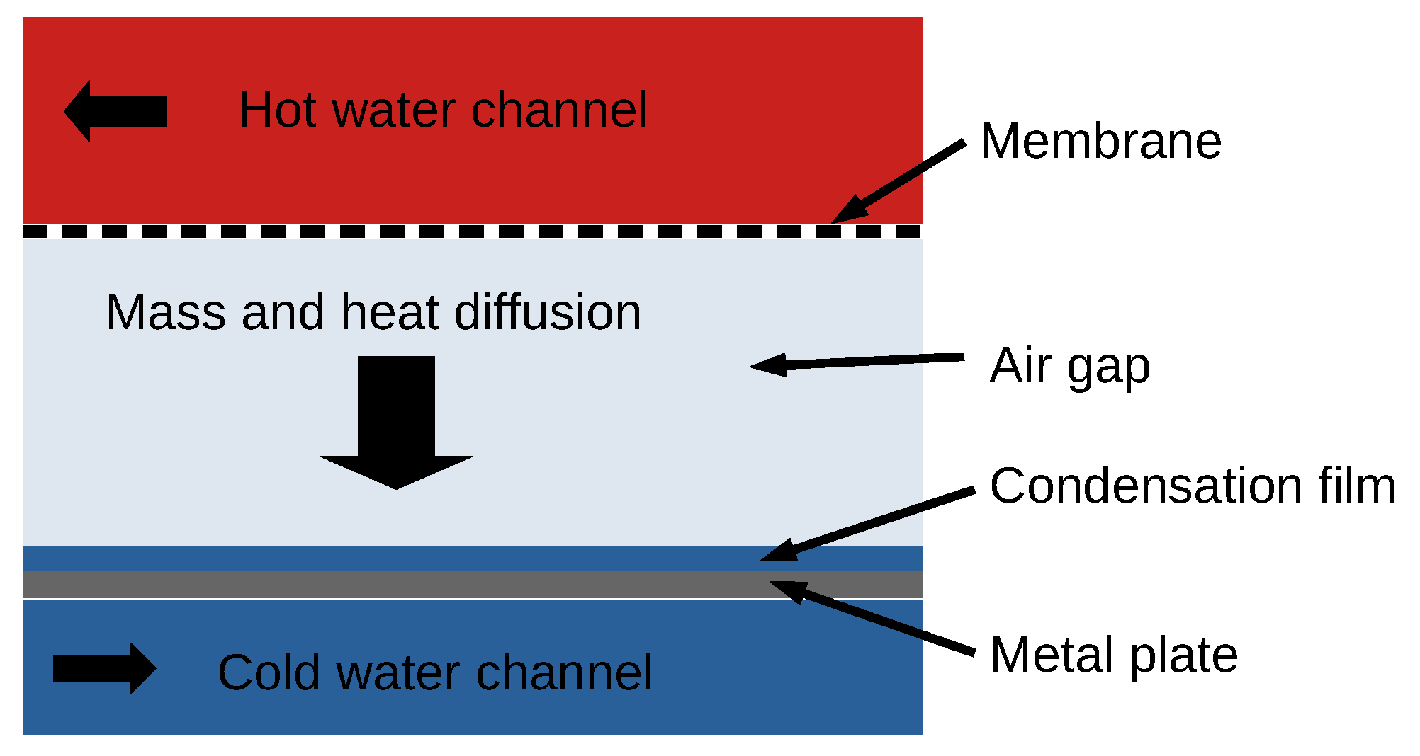
Figure 1.
Sketch of an AGMD module.
Figure 1.
Sketch of an AGMD module.
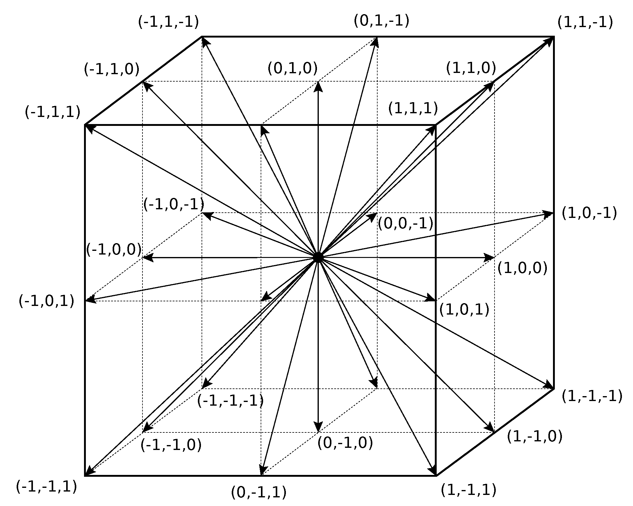
Figure 2.
D3Q27 lattice with 27 discrete velocities .
Figure 2.
D3Q27 lattice with 27 discrete velocities .
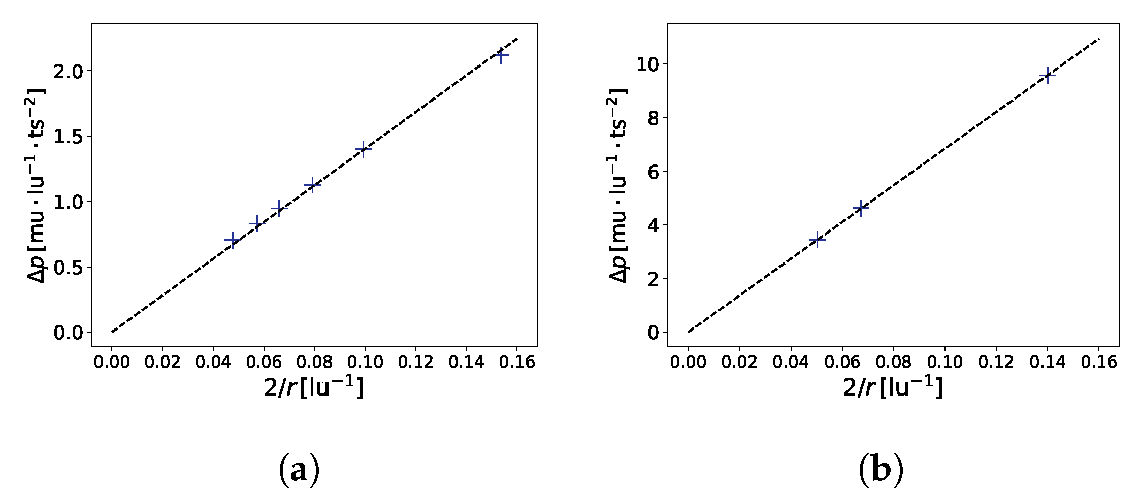
Figure 3.
Laplace law benchmark (). In (a), , , , where is the coefficient of determination. In (b), , , . Simulations were performed on a 100 × 100 × 100 domain.
Figure 3.
Laplace law benchmark (). In (a), , , , where is the coefficient of determination. In (b), , , . Simulations were performed on a 100 × 100 × 100 domain.
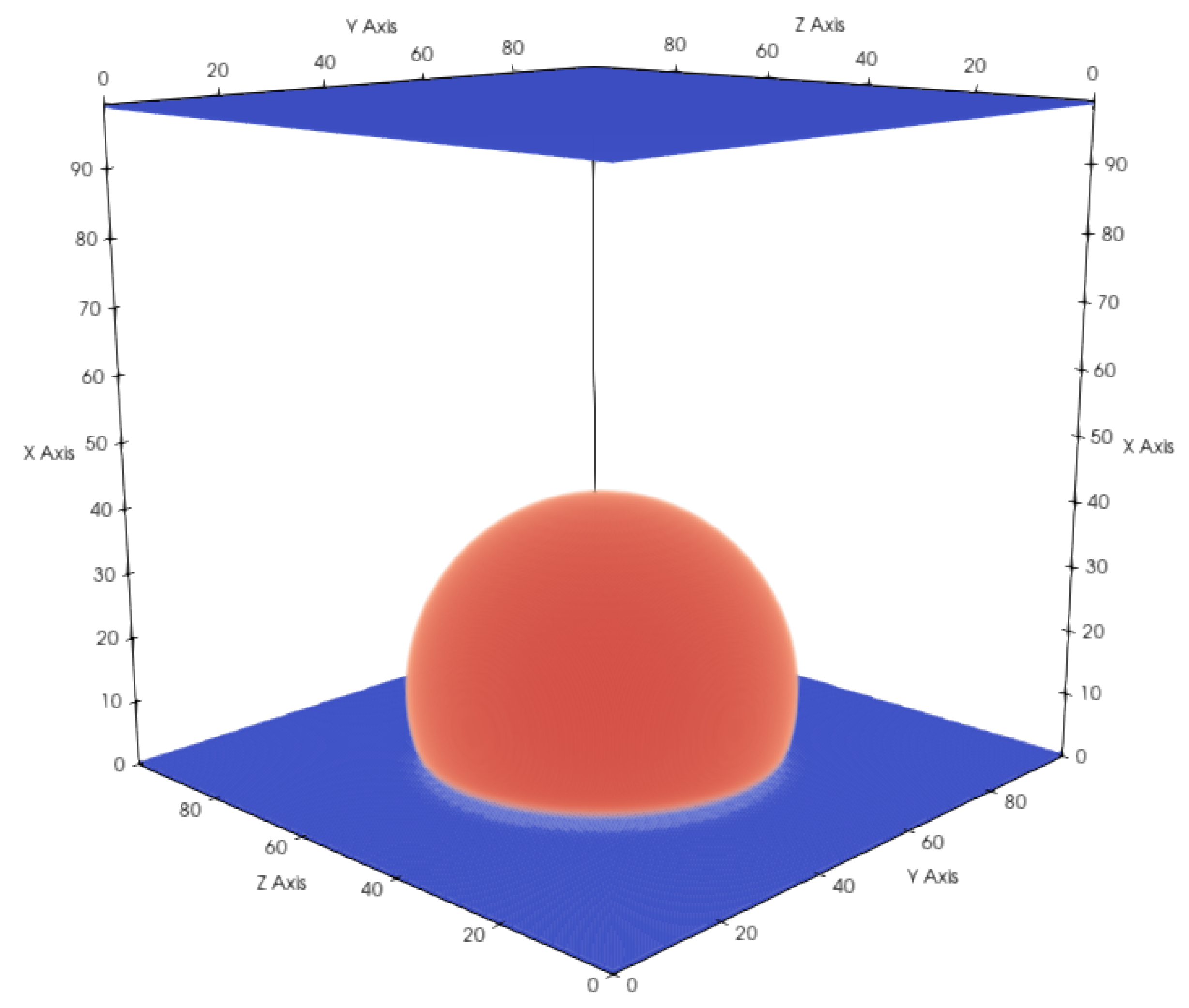
Figure 4.
Droplet on a flat hydrophobic surface with a total domain size of voxels. Gaseous phase is not shown for better visibility. Contact angle changes depending on the hydrophobicity, which can be controlled with and G. and result in a contact angle of .
Figure 4.
Droplet on a flat hydrophobic surface with a total domain size of voxels. Gaseous phase is not shown for better visibility. Contact angle changes depending on the hydrophobicity, which can be controlled with and G. and result in a contact angle of .
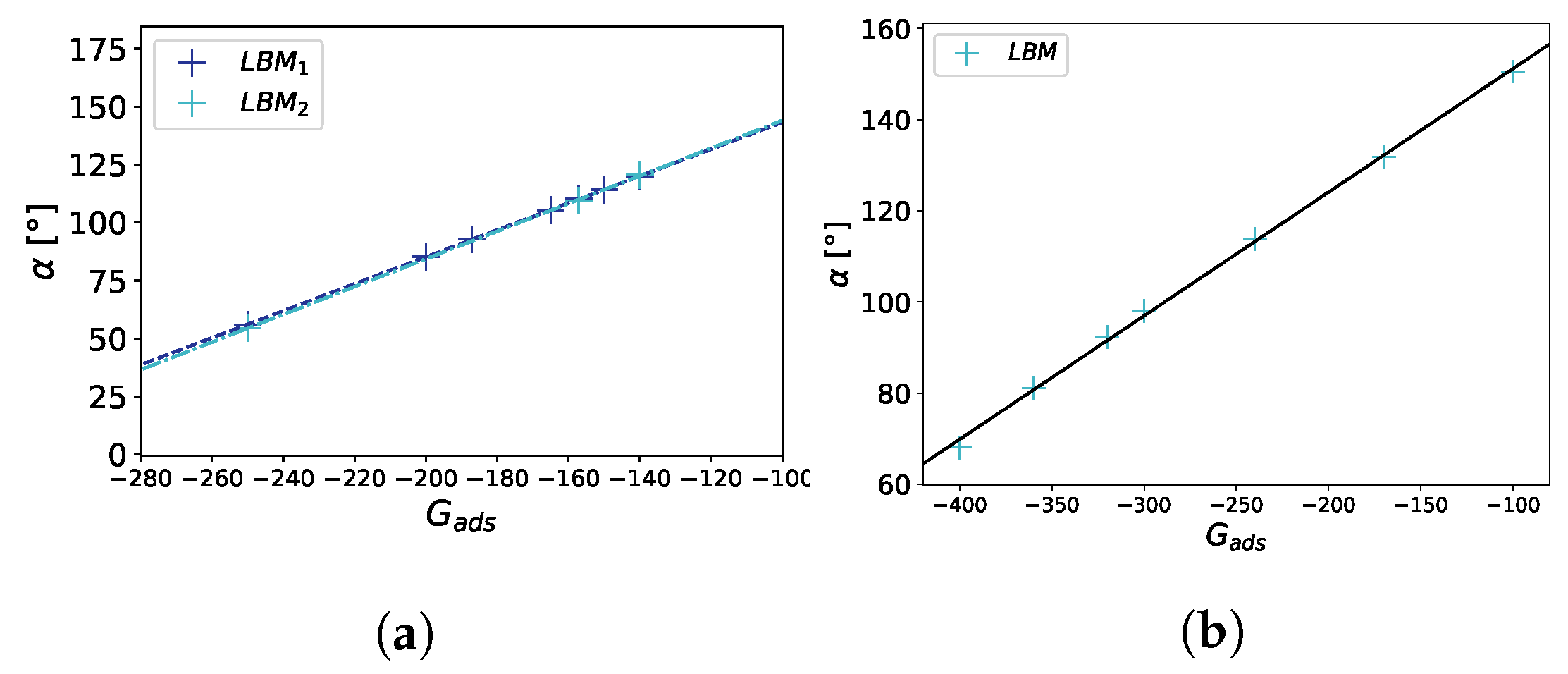
Figure 5.
Contact angle benchmark on a flat surface. The contact angle is plotted against the strength of the fluid–solid interaction . In (a), , , and correspond to the different droplet sizes in the LB simulation (, ). For a linear fit , we obtain for the two droplet sizes , , , , , , where is the coefficient of determination. In (b), . Simulations were performed on a 100 × 100 × 100 domain.
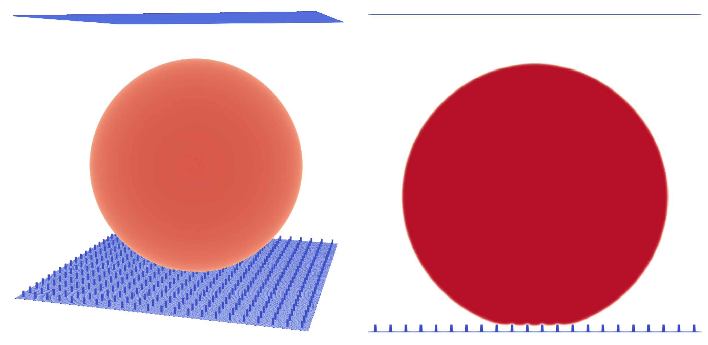
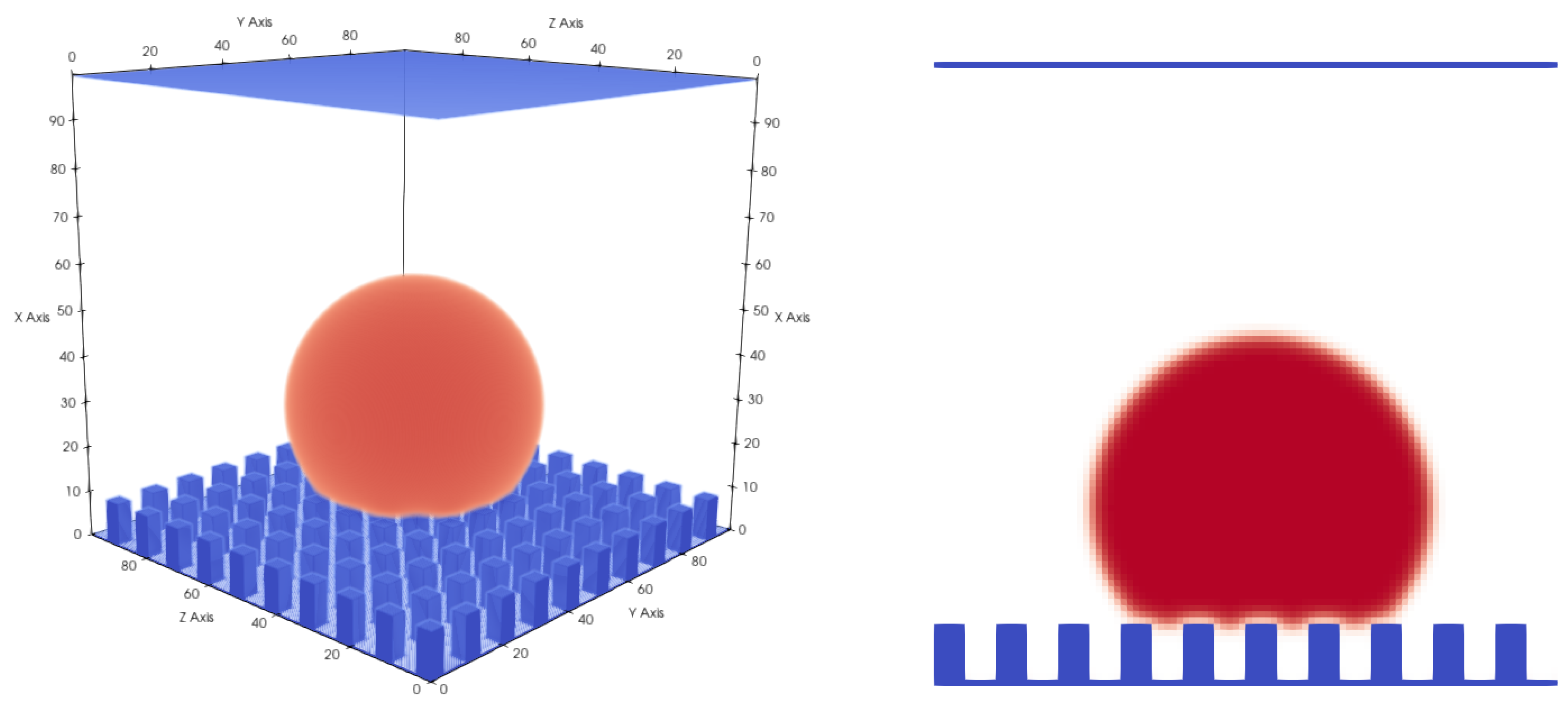
Figure 6.
Micro pillar structure with , pillar height , and . A droplet in the Cassie–Baxter state. Liquid phase is shown in red and micropillar structure is shown in blue.
Figure 6.
Micro pillar structure with , pillar height , and . A droplet in the Cassie–Baxter state. Liquid phase is shown in red and micropillar structure is shown in blue.
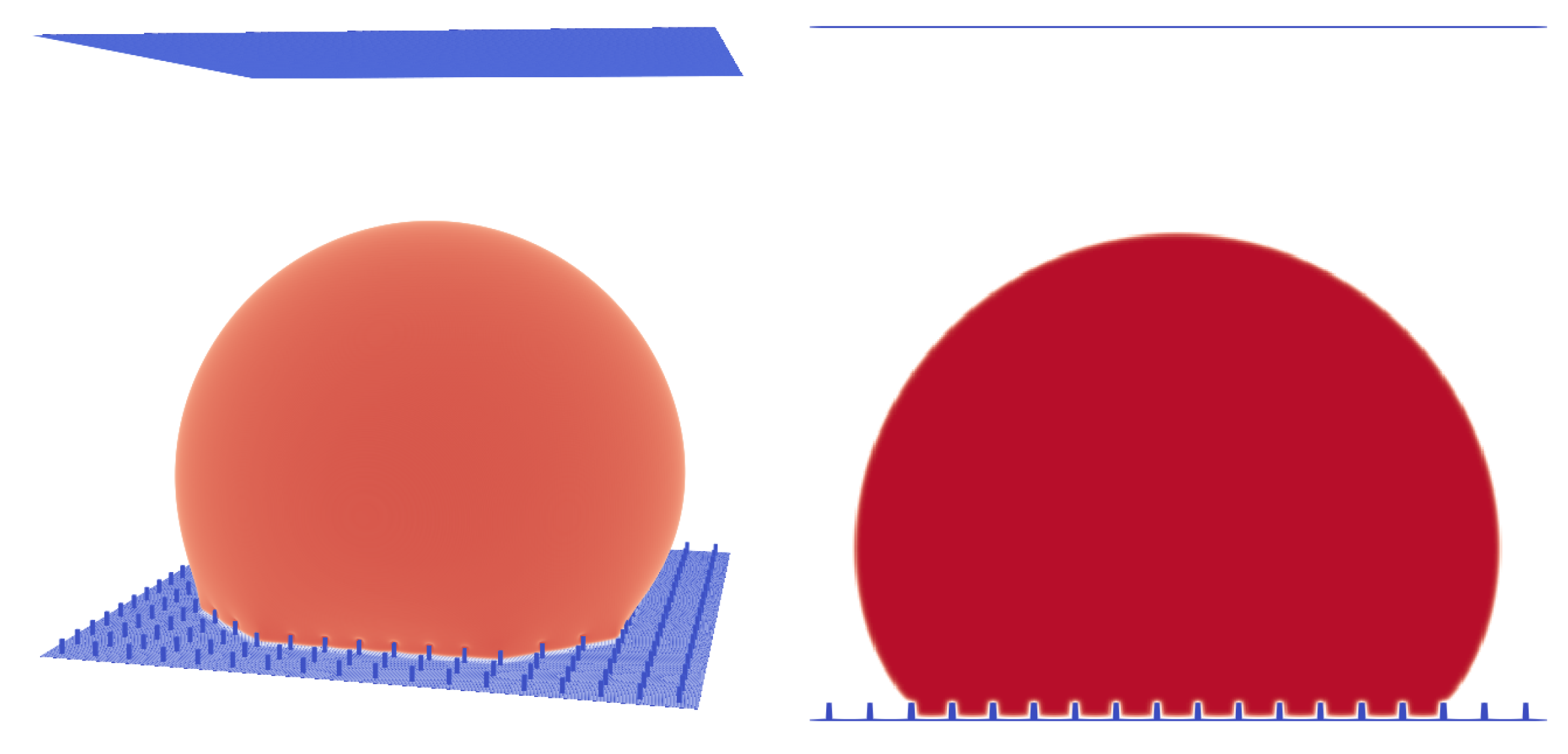
Figure 7.
Micro pillar structure with , pillar height , and . A droplet in the Wenzel state. Liquid phase is shown in red and micropillar structure is shown in blue.
Figure 7.
Micro pillar structure with , pillar height , and . A droplet in the Wenzel state. Liquid phase is shown in red and micropillar structure is shown in blue.
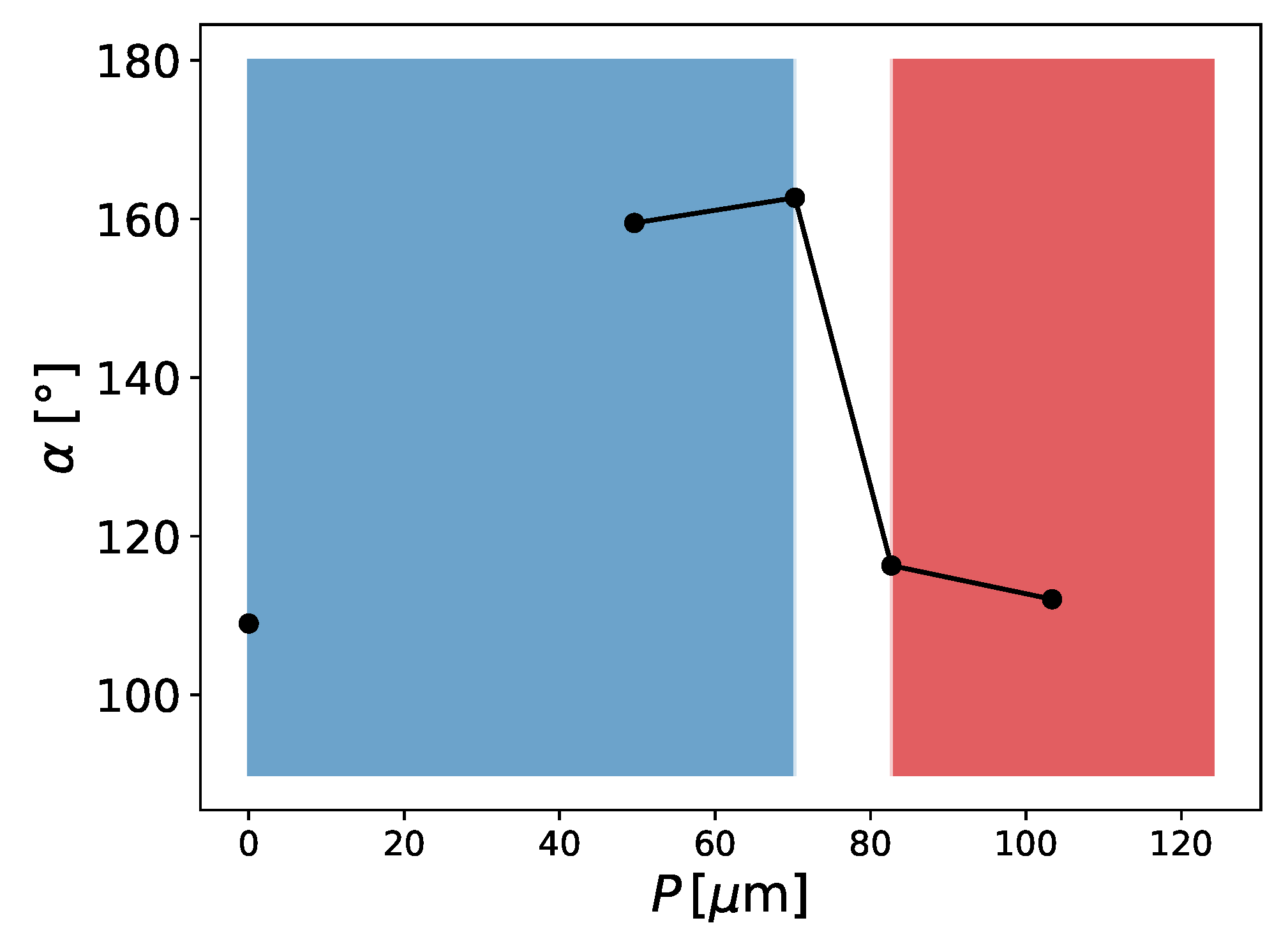
Figure 8.
Contact angle in dependence of the pitch between pillars (P). For the blue area, the droplet is in the Cassie–Baxter state and for the red area, the droplet is in the Wenzel state; , droplet volume is , , and .
Figure 8.
Contact angle in dependence of the pitch between pillars (P). For the blue area, the droplet is in the Cassie–Baxter state and for the red area, the droplet is in the Wenzel state; , droplet volume is , , and .
Figure 9.
Droplet on a rough hydrophobic surface in the Cassie–Baxter state, with a total domain size of voxels. Gaseous phase is not shown for better visibility. The roughness of the surface has an impact on the apparent contact angle, which in this case is (, , , , ).
Figure 9.
Droplet on a rough hydrophobic surface in the Cassie–Baxter state, with a total domain size of voxels. Gaseous phase is not shown for better visibility. The roughness of the surface has an impact on the apparent contact angle, which in this case is (, , , , ).
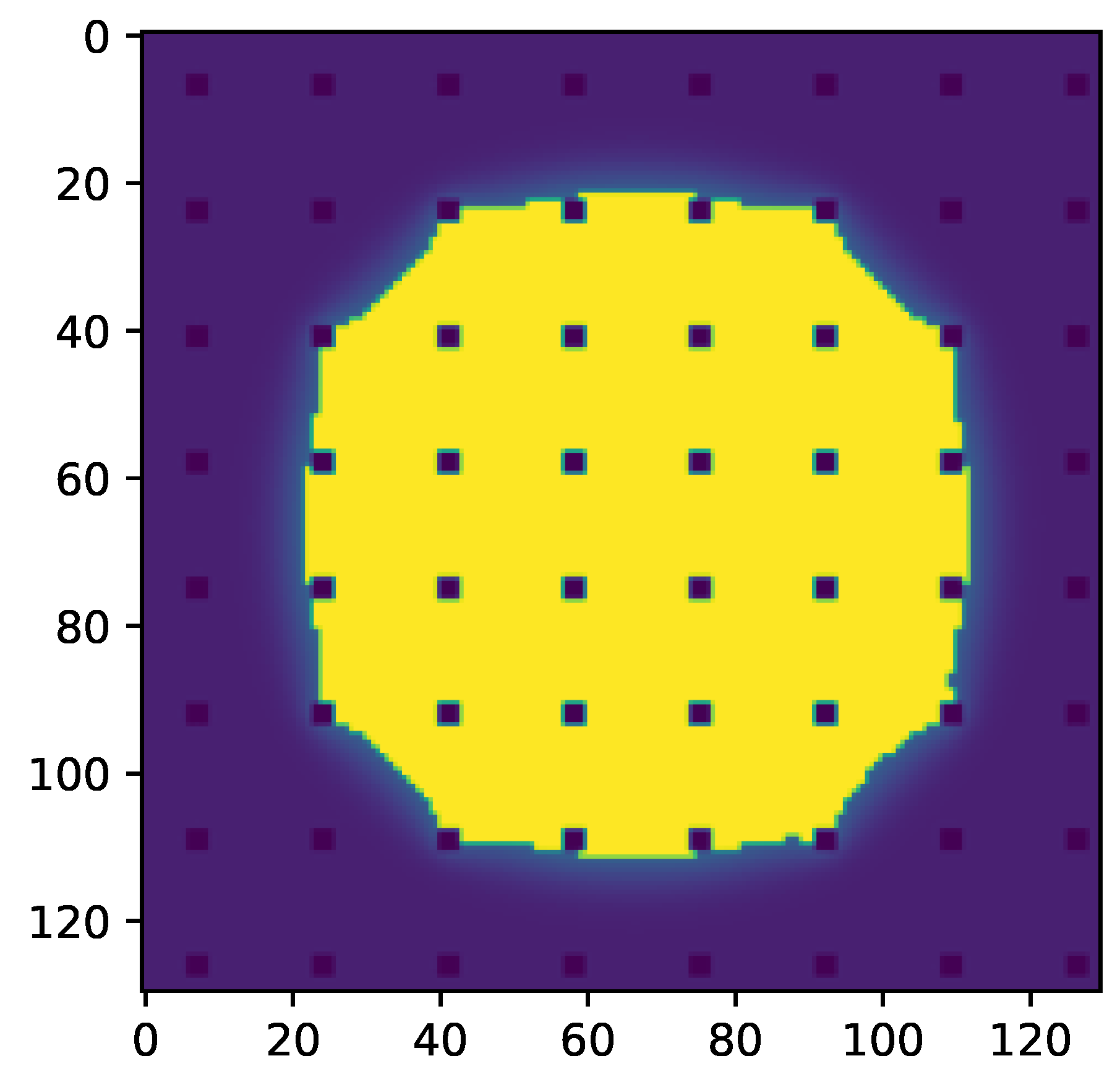
Figure 10.
Slice through the droplet parallel to the surface right above the micropillars of the results seen in
Figure 6. Liquid phase is shown in yellow and pillars are shown in dark blue. The yellow surface area can be used to calculate
.
Figure 10.
Slice through the droplet parallel to the surface right above the micropillars of the results seen in
Figure 6. Liquid phase is shown in yellow and pillars are shown in dark blue. The yellow surface area can be used to calculate
.
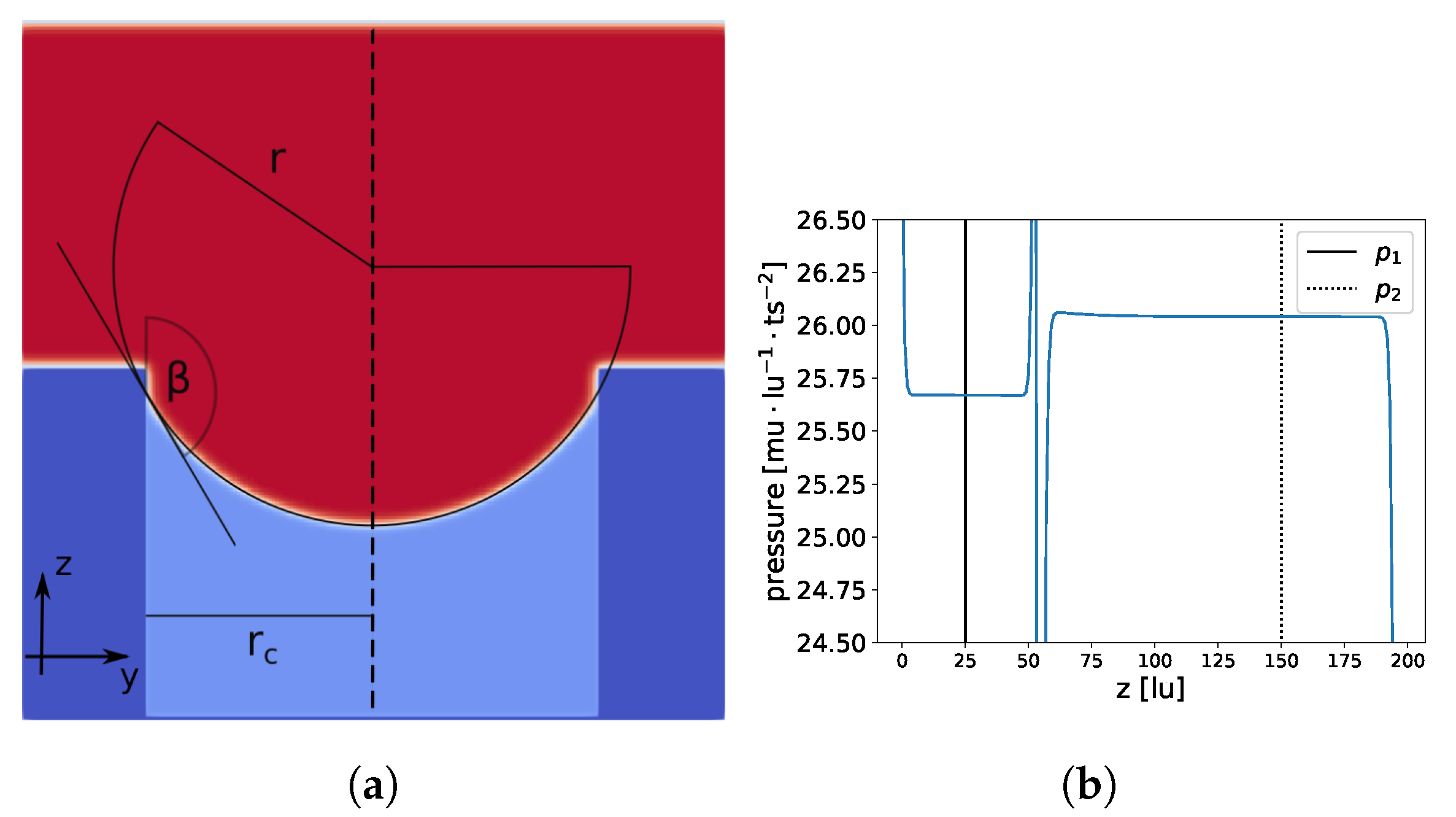
Figure 11.
Constant pressure gradient is applied along the z-axis (from bottom to top) in the full domain. Total domain size is lu and the pore radius is 64 lu. In (a), a slice at is shown; membrane material is dark blue, liquid is red, and gas is light blue. In (b), the pressure profile at the center of the cylindrical pore (dashed line in (a) at , ) is shown.
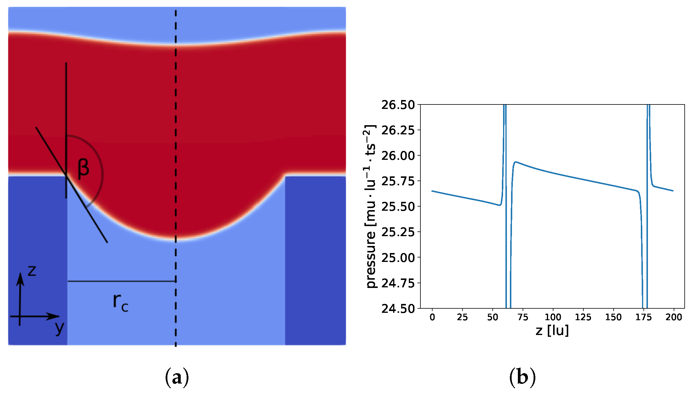
Figure 12.
Constant pressure in liquid and gas phases. Total domain size is lu and the pore radius is 64 lu. In (a), a slice at is shown; membrane material is dark blue, liquid is red, and gas is light blue. In (b), the pressure profile at the center of the cylindrical pore (dashed line in (a) at , ) is shown.
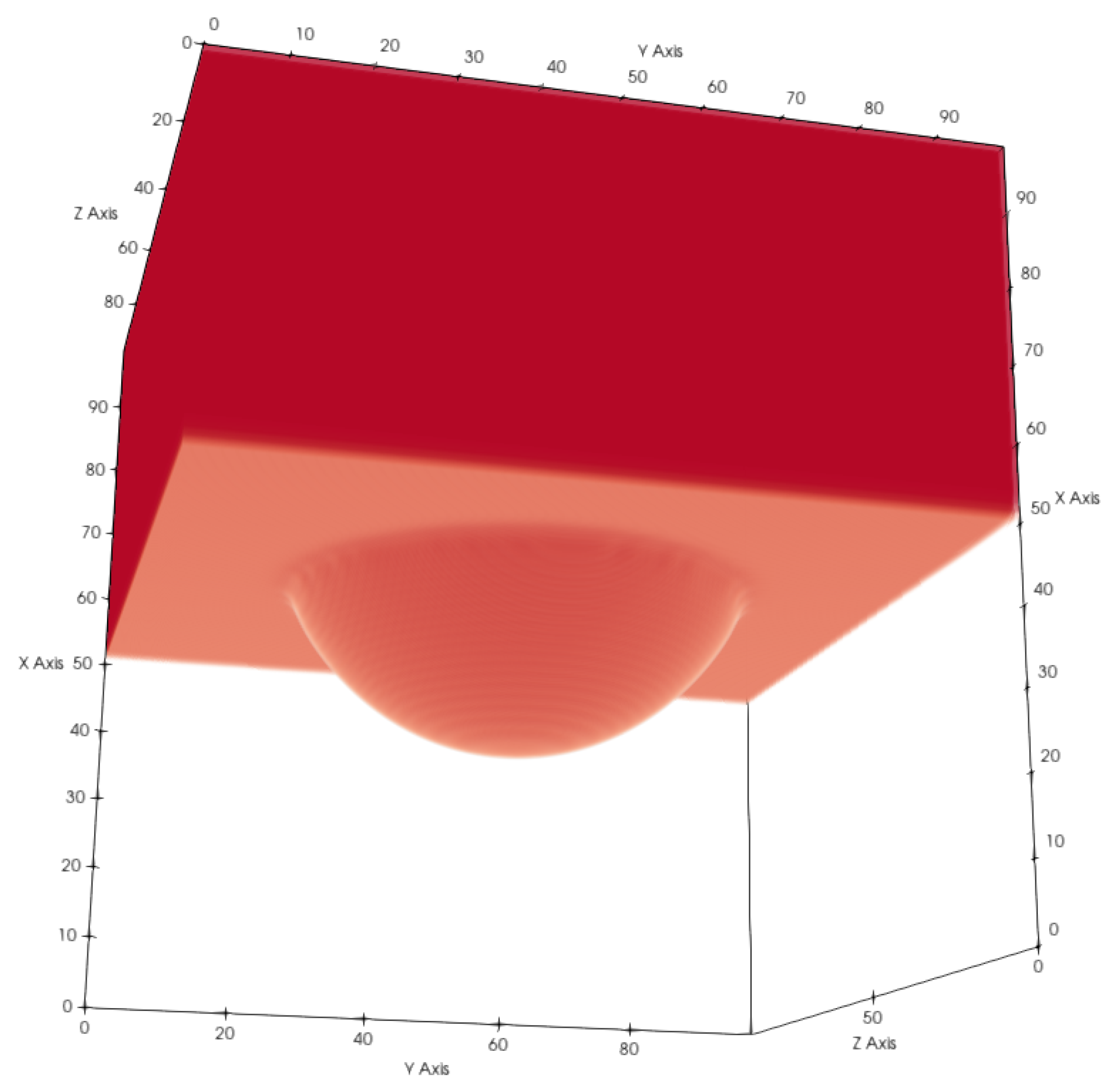
Figure 13.
Liquid (red) entering a cylindrical pore. Gaseous phase and solid voxels are not shown for better visibility. We chose for this test and .
Figure 13.
Liquid (red) entering a cylindrical pore. Gaseous phase and solid voxels are not shown for better visibility. We chose for this test and .
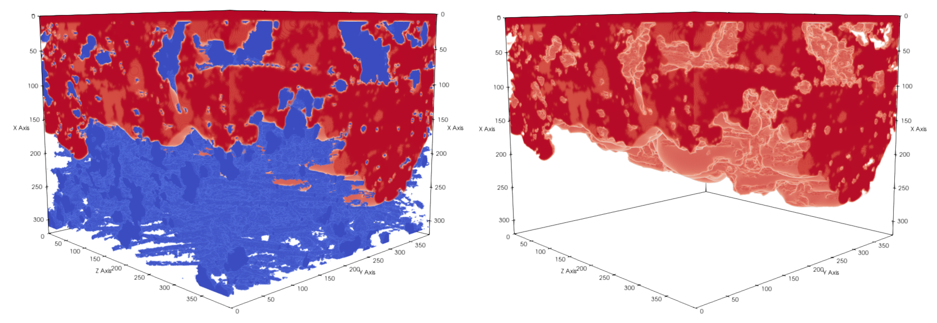
Figure 14.
Subsection of sample 3 with membrane dimensions . The pressure difference between the top and bottom sides of a membrane is . Membrane material is shown in blue and liquid in red. Liquid did not completely cross the membrane geometry.
Figure 14.
Subsection of sample 3 with membrane dimensions . The pressure difference between the top and bottom sides of a membrane is . Membrane material is shown in blue and liquid in red. Liquid did not completely cross the membrane geometry.
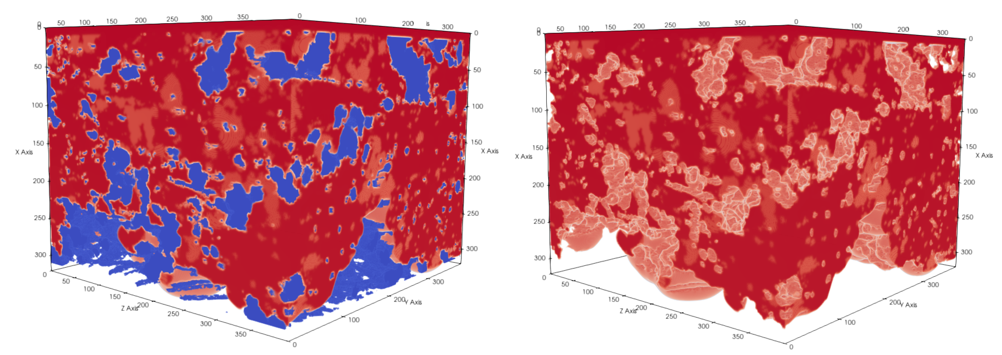
Figure 15.
Subsection of sample 3 with membrane dimensions . The pressure difference between the top and bottom sides of a membrane is . Membrane material is shown in blue and liquid in red. Liquid fully crossed the membrane geometry.
Figure 15.
Subsection of sample 3 with membrane dimensions . The pressure difference between the top and bottom sides of a membrane is . Membrane material is shown in blue and liquid in red. Liquid fully crossed the membrane geometry.
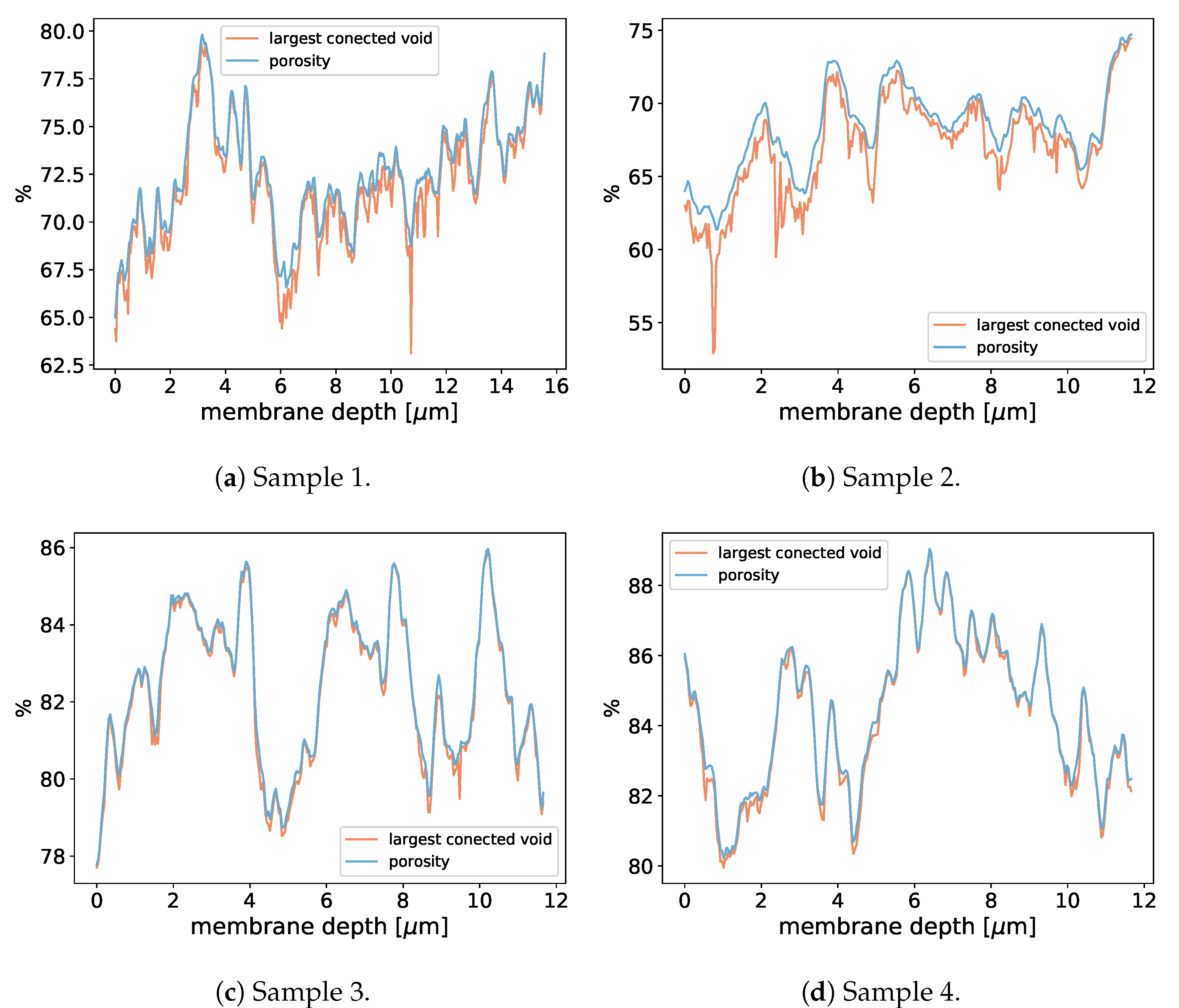
Figure 16.
Porosity in dependence of the membrane depth (
x-direction) for the the membrane subsamples used in
Table 4.
Figure 16.
Porosity in dependence of the membrane depth (
x-direction) for the the membrane subsamples used in
Table 4.
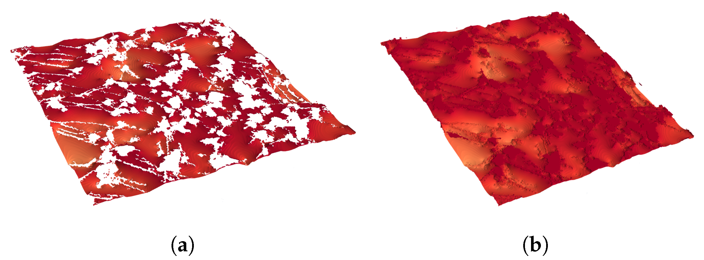
Figure 17.
Example of the liquid–gas contact area in (a) and the liquid surface area in (b).
Figure 17.
Example of the liquid–gas contact area in (a) and the liquid surface area in (b).
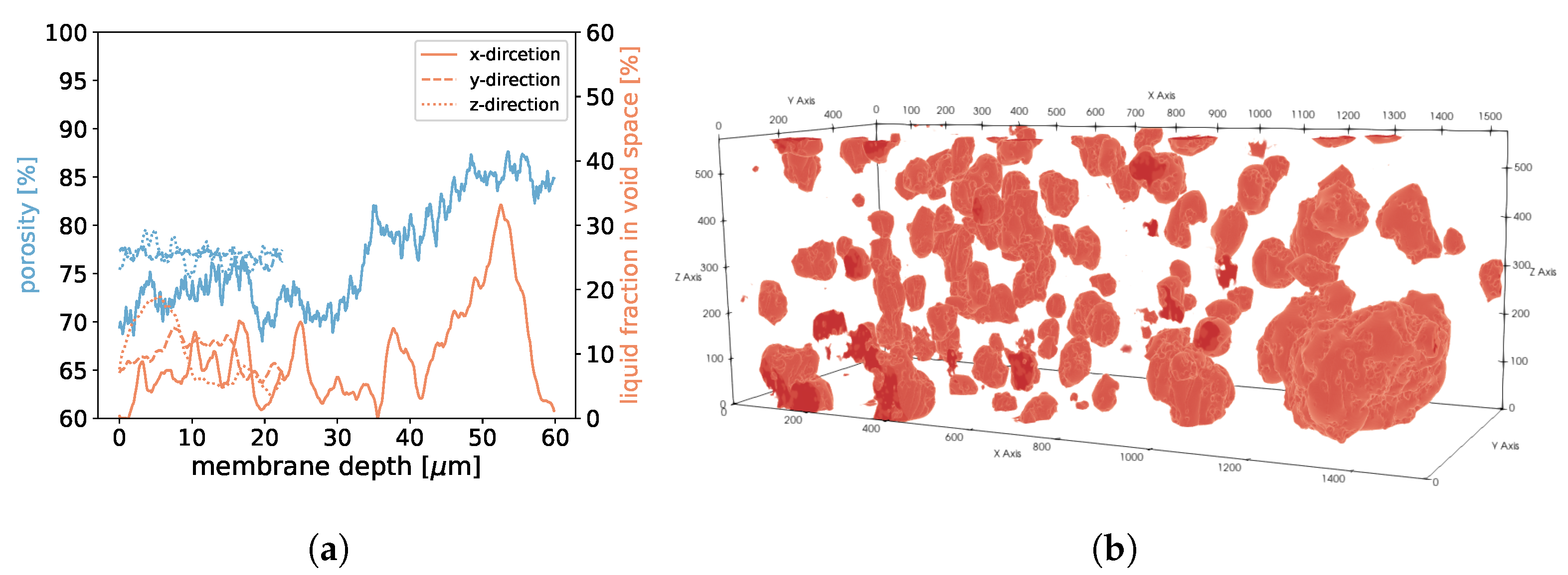
Figure 18.
In (
a), the porosities along the
x-,
y-, and
z-axes are shown for sample 1. Moreover, we display the fraction of void space that is occupied by liquid at a given membrane depth. In (
b), liquid droplets are shown in red for sample 1. Gaseous phase and membrane material is not shown for better visibility. It should be noted that the convergence criterion in Equation (
11) only reached
.
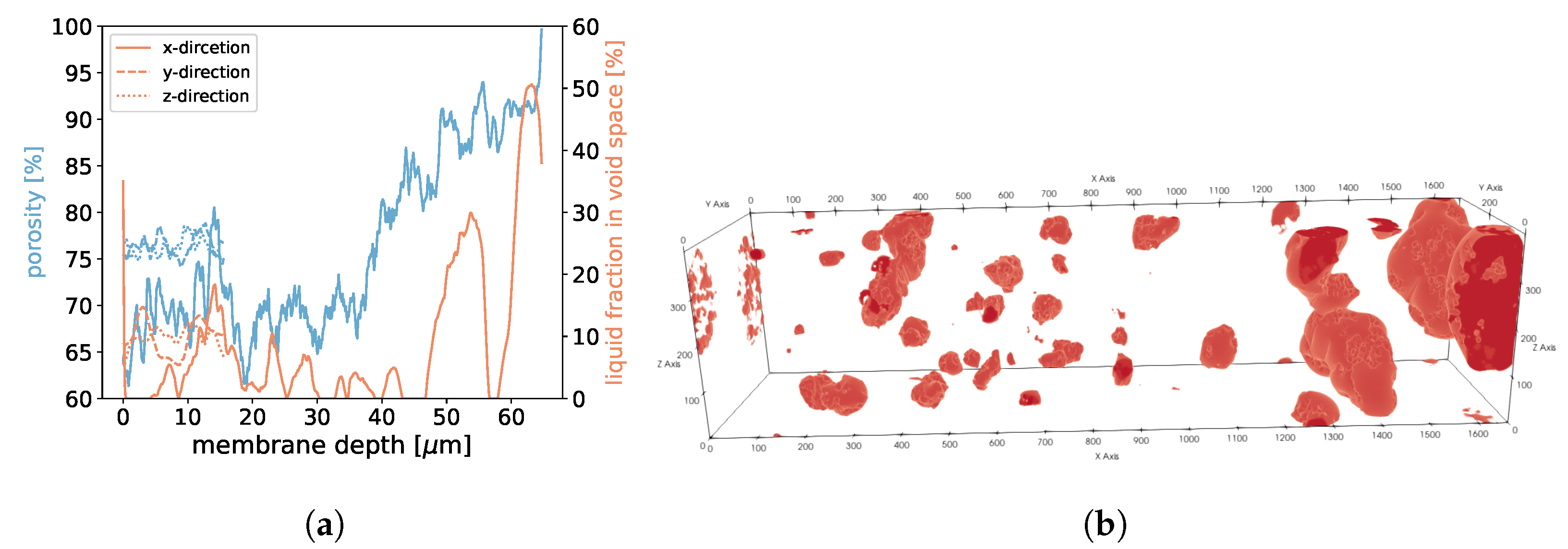
Figure 19.
In (
a), the porosities along the
x-,
y-, and
z-axes are shown for sample 2. Moreover, we display the fraction of void space that is occupied by liquid at a given membrane depth. In (
b), liquid droplets are shown in red for sample 2. Gaseous phase and membrane material is not shown for better visibility. It should be noted that the convergence criterion in Equation (
11) only reached
.
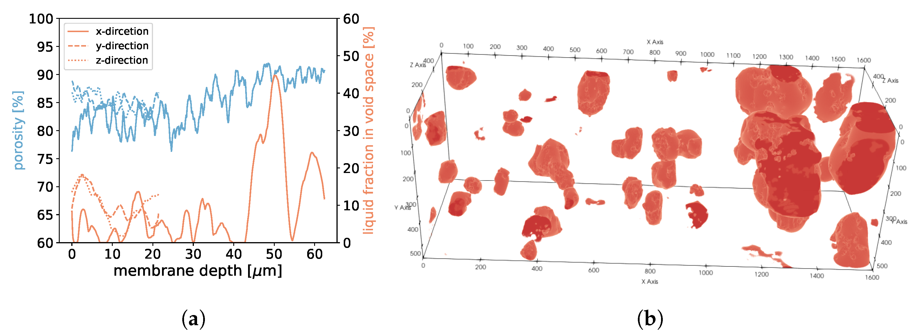
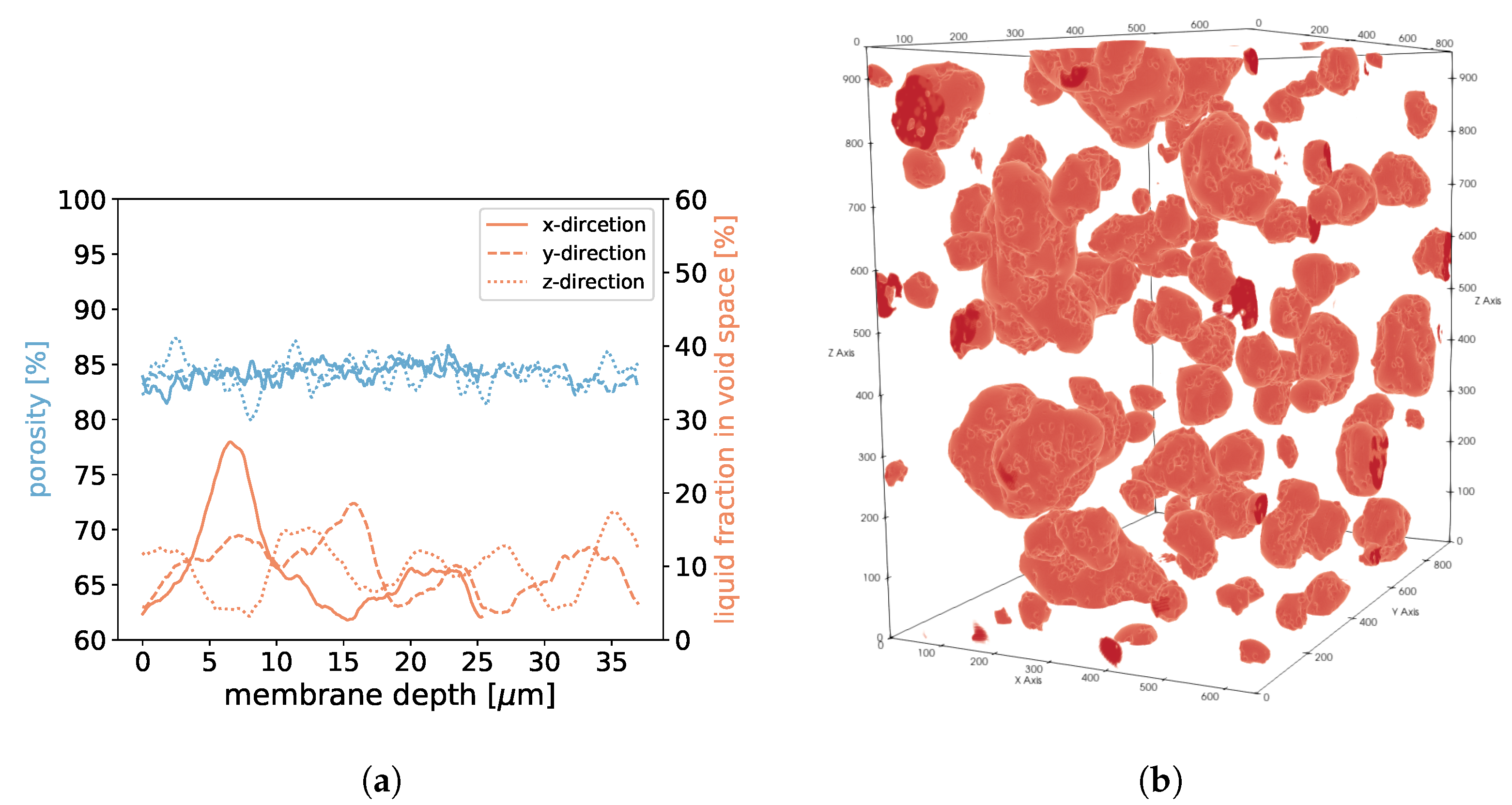
Figure 20.
In (a), the porosities along the x-, y-, and z-axes are shown for sample 3. Moreover, we display the fraction of void space that is occupied by liquid at a given membrane depth. In (b), liquid droplets are shown in red for sample 3. Gaseous phase and membrane material is not shown for better visibility.
Figure 21.
In (
a), the porosities along the
x-,
y-, and
z-axes are shown for sample 4. Moreover, we display the fraction of void space that is occupied by liquid at a given membrane depth. In (
b), liquid droplets are shown in red for sample 4. Gaseous phase and membrane material is not shown for better visibility. It should be noted that the convergence criterion in Equation (
11) only reached
.
Table 1.
3D membrane geometries obtained by Cramer et al. [
12].
Table 1.
3D membrane geometries obtained by Cramer et al. [
12].
| Sample | Membrane | Manufacturer | Pore Diameter |
Sample Dimensions ()
|
|---|
| | | | [] | [] |
[Voxels]
|
|---|
| 1 | FGLP14250 | Merck Millipore | 0.2 | 59.85
| |
| 2 | Gore
| Gore | 0.22 | | |
| 3 | FHLP14250 | Merck Millipore | 0.45 | | |
| 4 | FGLP14250 | Merck Millipore | 0.2 | | |
Table 2.
Summary of membrane and fluid properties.
Table 2.
Summary of membrane and fluid properties.
| | LB Units | SI Units | Remark |
|---|
| 1028 | 998.861 | pure water, 1 bar, 16.5 C |
| 53 | 1.204 | 1 bar, 16.5 C |
| 975 | 997.657 | |
| 19.4 | 829.619 | |
| 171.33 | Pa·s | 1 bar, 16.5 C |
| 8.83 | Pa·s | 1 bar, 16.5 C |
| 19 | 60 | |
| 1 | m | |
| 1 | s | |
| c | 1 | 168.5 m/s | |
| La | 24,424 | 24,424 | 1 bar, 16.5 C |
| 68 | 0.073 N/m | pure water, 1 bar, 16.5 C |
| Bo | | | |
Table 3.
The apparent contact angle on a rough surface is compared to the predictions using the Cassie–Baxter (CB) and Wenzel equations. Values in parentheses show the deviations from the LB simulations as percentages.
Table 3.
The apparent contact angle on a rough surface is compared to the predictions using the Cassie–Baxter (CB) and Wenzel equations. Values in parentheses show the deviations from the LB simulations as percentages.
| State | Size [voxel] | [voxel] | P | H | [] Flat LBM | [] Rough LBM | [] | | [] | | |
|---|
| CB | 100 × 100 × 100 | | 10 | 10 | | | | | | | - |
| | | | | | | | () | | () | | |
| CB | 100 × 100 × 100 | | 10 | 10 | | | | | | | - |
| | | | | | | | () | | () | | |
| CB | 100 × 100 × 100 | | 10 | 10 | | | | | | | - |
| | | | | | | | () | | () | | |
| CB | 121 × 175 × 175 | | 20 | 15 | | | - | - | | | - |
| | | | | | | | | | () | | |
| CB | 320 × 380 × 380 | | 20 | 15 | 109 | | | | | | - |
| | | | | | | | () | | () | | |
| CB | 342 × 384 × 384 | | 12 | 8 | 109 | | | | | | - |
| | | | | | | | () | | () | | |
| CB | 357 × 374 × 374 | | 17 | 8 | 109 | | | | | | - |
| | | | | | | | () | | () | | |
| Wenzel | 340 × 360 × 360 | | 20 | 8 | 109 | | - | - | | - | |
| | | | | | | | | | () | | |
| Wenzel | 357 × 374 × 374 | | 25 | 8 | 109 | | - | - | | - | |
| | | | | | | | | | () | | |
Table 4.
Liquid entry depth in the x-direction and pressure differences for multiple membrane subsamples obtained from the LB simulations are compared to the liquid entry pressures from the experiments. Predictions are in close agreement with the experimental values.
Table 4.
Liquid entry depth in the x-direction and pressure differences for multiple membrane subsamples obtained from the LB simulations are compared to the liquid entry pressures from the experiments. Predictions are in close agreement with the experimental values.
| Sample | Membrane Dimensions () | | Liquid Entry Depth in x | LEP Experiments [33] |
|---|
| | [] | [voxels] | [bar] | [] | [bar] |
|---|
| 1 | | | 3.112 | > (breakthrough) | 2.8 |
| | | | 2.510 | > (breakthrough) | (from manufacturer) |
| | | | 1.912 | | |
| | | | 0.732 | | |
| | | | 0.182 | | |
| 2 | | | 2.510 | > (breakthrough) | |
| | | | 1.912 | | |
| | | | 2.21 | | |
| | | | 1.912 | | |
| | | | 1.320 | | |
| | | | 0.182 | | |
| 3 | | | 1.912 | > (breakthrough) | |
| | | | 1.320 | | |
| | | | 0.182 | | |
| 4 | | | 1.912 | > (breakthrough) | 2.8 |
| | | | 1.320 | > (breakthrough) | (from manufacturer) |
| | | | 1.025 | | |
| | | | 0.182 | | |
Table 5.
Liquid–gas contact area. Membrane subsample size is for sample 1, 3, and 4 and for sample 2. . is the liquid–gas contact surface area, is the total surface area of the liquid, and is the area of the membrane cross-section. The velocity v is introduced parallel to the membrane plane and at a distance of from the membrane plane.
| Sample | v [cm/s] | Pillars | [%] | [%] | [%] |
|---|
| 1 | 0.0 | no | 51.96 | 64.48 | 124.10 |
| 2 | 0.0 | no | 51.3 | 63.99 | 124.74 |
| 3 | 0.0 | no | 62.4 | 76.96 | 123.33 |
| 3 | 1.7 | no | 62.4 | 76.96 | 123.33 |
| 3 | 0.0 | yes | 44.24 | 71.73 | 162.14 |
| 3 | 1.7 | yes | 44.25 | 71.74 | 162.12 |
| 4 | 0.0 | no | 64.08 | 81.88 | 127.78 |
Table 6.
Surface area between liquid and gaseous phases () compared to the surface area of a sphere with the same volume () and the total surface area of all droplets, which includes the surface area of the droplets that are in contact with the membrane material ().
Table 6.
Surface area between liquid and gaseous phases () compared to the surface area of a sphere with the same volume () and the total surface area of all droplets, which includes the surface area of the droplets that are in contact with the membrane material ().
| Sample | Domain Dimensions | [%] | [%] | [%] | [%] | [%] | [%] |
|---|
| 1 | 1535 × 575 × 575 | 7.61 | 69.25 | 23.14 | 48.72 | 328.84 | 674.96 |
| 2 | 1660 × 400 × 400 | 7.57 | 68.8 | 23.63 | 57.66 | 222.17 | 385.31 |
| 3 | 1601 × 550 × 550 | 8.42 | 76.62 | 14.96 | 60.53 | 239.15 | 395.09 |
| 4 | 650 × 950 × 950 | 8.33 | 75.9 | 15.77 | 53.29 | 350.47 | 657.66 |


