1. Introduction and Previous Studies
Ocean-going vessels must have a reliable power supply. It is hard to imagine nuclear energy becoming interesting if only merchant ships are considered. Fuel cell technology is not yet mature for such power. The most efficient process is still diesel. These facts are undisputed.
Regardless of which process is used in the internal combustion engine, HC compounds are consumed, and the emission of water vapor and carbon dioxide (CO2) is the side effect. The emission of a certain amount of carbon dioxide cannot be avoided.
In many countries around the world, various methods or measures have been introduced to reduce or minimize carbon dioxide emissions and other harmful substances in ports and coastal waters in general. One such measure is reduction in ship speed, often referred to as “slow steaming”. Slow steaming and its effect on fuel and carbon dioxide emission reduction has been thoroughly investigated [
1,
2,
3,
4,
5]. Tezdogan, T. et al. evaluated the impact of a slow steaming approach on reducing the fuel consumption of a container ship sailing in a high sea state. The key objective was to estimate the increase in effective power and fuel consumption due to its operation in regular and irregular head seas. Analyses were performed at design and slow speed, for a range of wave conditions in normal seas, and for three different sea states in irregular seas. The increase in water resistance was a key parameter in determining power and fuel consumption increase. Degiuli, N. et al. analyzed the impact of slow steaming on reducing CO
2 emissions in the Mediterranean Sea for a container ship model using different fuel types and sailing in different sea conditions. Again, the increase in water resistance was determined using flow theory, resulting in an increase in power and fuel consumption. Energetic and environmental impacts of slow steaming on a container ship model sailing from Shanghai to Hamburg were analyzed in a paper written by Gospić, I. et al. The same method was used, and the results showed that fuel consumption and carbon dioxide emissions could be significantly reduced. An overview of the environmental and economic benefits of slow steaming was reported by Zanne, M., et al. The paper reviewed existing studies on slow steaming and listed other available and already applicable solutions, such as renewable energy applications, waste heat recovery, etc. A study by Goicoechea, N. and Abadie, M.L. reported on the cash flow for a typical container ship. It found that the optimal speed depended on the size of the ship, and several variables such as fuel prices, freight rates, and other voyage costs. The effectiveness of slow steaming in reducing pollutant emissions has been the subject of numerous studies, but most have utilized data on main engine performance.
One approach to reducing pollutant emissions or improving economic outcomes is to optimize speed throughout the trip. Such an economic approach was used in [
6], where the authors considered optimal speed instead of slow speed.
Lighter fractions of crude oil or even methane or methanol, instead of the typical heavy fuel oil (HFO), would lead to a reduction in carbon emissions [
7]. There are several papers dealing with the effects of the operating conditions of the slow turning main diesel engine on fuel consumption and carbon dioxide emission [
8,
9,
10,
11,
12]. Glujić et al. and Radonja et al. studied fuel consumption of diesel engines as a function of cooling water temperature. Pelić et al. investigated the effects of early closure of the intake valve and split injection on fuel consumption and pollutant emissions of medium speed diesel engines. The work of Vorkapić et al. found that their proposed framework was feasible and widely applicable in the marine industry. The novelty was that the proposed framework used on-board data processing, and was integrated with the existing ship monitoring, decision-making, and reporting system, thus, meeting the requirements for ease of application. A ship monitoring system should be able to reduce energy consumption and harmful gas emissions.
Several papers have used data collected from ships to make a comprehensive study of their impact on air when operating in ports [
13,
14,
15]. The studies analyzed emissions of carbon dioxide and other harmful gases for one year. Although data collected on board ships can be misleading, they have been used in research [
16,
17] to create a ship monitoring model for optimal fuel consumption.
Some novel technologies have been addressed in [
18,
19]. Pelić, Mrakovčić, Medica-Viola and Valčić analyzed the implementation of a photovoltaic plant on board ships and its effect on fuel consumption and the emission of harmful gases. Pelić, Mrakovčić, Bukovac and Valčić developed a numerical model and confirmed its usability for research purposes in diesel engine optimization. Xing, H. et al. [
20] provided a comprehensive overview of technical and operational measures to reduce CO
2 from ships. A complete research overview of decarbonization methods used in the last 20 years was presented by Romano, A., et al. [
21]. They reported that one way to reduce carbon emissions from ships would be to use alternative propulsion systems that run on alternative fuels. A technical analysis of the engineering considerations for using such fuels was described by McKinlay, J.C. et al. [
22]. Unfortunately, it was reported that the effect could only be predicted in 30% of those measures, and in 70% of measures, it was not possible to predict the outcome. It is well known, in the history of humanity, that technological processes have been introduced, termed as revolutions. After a certain period following each revolution, along with positive effects, certain negative effects have also been observed. Our history is full of such examples [
23].
Zanne, M. et al. [
4] states: “As different studies show, majority of customers have positively accepted slow steaming, although some individual customers might lose their market position due to longer delivery times and costs connected to this. Alternative approaches do not affect the operating speed of the ship as slow steaming does, and many believe that slow steaming could be refused as soon as maritime market recovers or can become regulated if external benefits are recognized in their entirety. The future of slow steaming will mostly rely on market situation, fuel prices as well as on the supply chain requirements and the oscillations in vessel’s operating cost. Considering the fact that the environmental concerns will not vanish, but instead might then become even more emphasized, slow steaming will probably not be an optimal solution when global economy revives.” Nevertheless, some coastal countries limit vessel speed in their waters to 12 knots up to a distance of 200 NM from shore, to reduce harmful emissions.
This is a universal measure, meaning that any vessel, regardless of engine type or mode of operation, must comply with these regulations. The aim of this paper is to investigate how a speed reduction to 12 knots affects total fuel consumption. It may seem quite obvious, because it is logical that lower speed leads to lower consumption. If only main engine consumption was taken into consideration, this statement would be correct, but the answer is not as clear when necessary electrical energy and steam generation are considered. The majority of studies previously mentioned only used main engine power, fuel consumption and harmful gases emission data, without taking into account other fuel consumers. In some cases, these data should not be excluded.
The analysis of this paper was conducted on a NorControl, Kongsberg, Norway engine room simulator for different types of main engines and modes of operation. A flow meter was not used on the main engine fuel system to measure fuel consumption; instead, flows from the appropriate service tanks to all consumers were measured.
The use of nautical and engineering simulators in scientific research is not new, and is much simpler and less expensive compared with traditional on-board measurement [
24,
25,
26,
27,
28,
29,
30,
31,
32,
33,
34]. On-board measurement means that investigators use data of at least questionable quality and validity as it is collected by crew members, or data collected by an automated data collection system. Generally, flow meters provide the best readings, but they are rarely installed in fuel supply lines of auxiliary boilers and diesel generators.
2. Description of the Ship and the Engine Room Models and Modes of Operation
The simulation was carried out on several ship and engine room models or their operation. The models were created by the world-renowned and respected manufacturer of computerized engine management systems and engine room simulators, the Norwegian company NorControl.
Engine room models were used in this research, both with slow turning and cross-head, large diesel engines. Why were models with medium-speed diesel engines, gas turbines, or electric propulsion, not used? The answer lies in statistical data: 95% or more ships still have slow turning diesel propulsion, based on the total power of the engines or the displacement of these ships. The ownerships of companies such as MAN-B&W, New Sultzer and Wartsila are changing, and it is not necessary to deal with it, but their production covers most of the world’s commercial shipping fleet.
Simulations were performed on a model of a very large crude oil carrier (VLCC) with a slow-speed MAN-B&W five-cylinder (5MC90) main engine (ME) giving a speed of 15 knots. The electric power plant of a VLCC has two diesel generators (DG), a turbogenerator (TG) that uses the steam generated in an exhaust steam generator, and a shaft generator (SG) that can be operated as an electric motor when it transfers its power to the propeller shaft. The ship has a large (HFO) oil-fired steam generator. The electric power plant is fully automated. The ‘stand-by’ generator starts and cuts-in when the network power demand is increased, and cuts-out and stops when power is decreased. Steam production is automated too. When the exhaust generator’s production is insufficient, the oil-fired unit automatically turns on. The number of revolutions of the main engine is set at one of three control positions. The difficulty is that the control accuracy of the number of revolutions is quite coarse.
The engine room simulator is an exact replica of the real computer management system used on board. There are two remote control boards: engine control room and bridge control room. The engine control room usually has more options: precision control, displays, management and regulation. There are also twelve logbooks with six channels to record almost any parameter. The recording starts when the tag of the parameter is inserted, and continues for as long as the simulation lasts.
Several modes of operation were used in the simulation, and there was a difference in whether the ship included the cargo or used the turbo and the shaft generator. The first mode of operation for this particular engine room was to run the main engine at maximum power, i.e., maximum continuous rating (MCR), and with the shaft generator and TG on. The diesel generators were not in operation.
The second mode of operation for the same engine room was to operate the main engine at 60% of maximum power
1 with the ship speed reduced to 11.89 NM and the same distribution of power generation. Why was this important? The TG uses the steam produced in the exhaust boiler, and there was a possibility that there would not be enough steam due to the lack of exhaust. The result may be increased overall fuel consumption because one or more diesel generators were required on the grid and because the fuel boiler was started automatically.
The third mode of operation for the same engine room was to operate the main engine at 60% of maximum power (ship speed of 11.89 NM), but the required power was generated by a TG and one of the diesel generators.
The fourth mode of operation for the same engine room was to operate the main engine at 60% of the maximum power (ship speed of 11.89 NM), but the required electric power was generated only by the shaft generator. All other electrical generators, the TG and the diesel generators, were shut down.
The first row of
Table 1 lists the abbreviations for the main engine and the electricity generators. In the following rows, the percentage of the maximum continuous power of the main engine and the configuration of the electric power plant, are given.
Two other scenarios were applied to a different ship and engine room model: a container ship with an RT-Flex 82C L11 engine. This is a very large engine that enables a much higher speed, compared with the previous model. The power plant has three diesel generators, a TG that uses steam generated in an exhaust steam generator, and a shaft generator that can be operated as an electric motor when it transfers its power to the propeller shaft. There is also an oil-fired steam generator (HFO). The complete power plant is very similar to the first one, but has one additional diesel generator because of occasional high-power demand. Due to the high rated power of this engine, a power reduction to about 40% was necessary to reach the limited speed of 12 knots.
Two modes of operation were considered for the container ship. The first mode was the main engine at maximum power, the shaft generator in power take in (PTI) mode transferring additional power to the shaft and the TG; none of the diesel generators were operating. The second mode of operation was the main engine running at about 40% of power (speed of 11.92 NM). The electrical power was only generated by the TG; all diesel generators and the shaft were out of service. The abbreviations in
Table 2 are the same as in
Table 1.
In all modes, electric power generation and SG working in PTI mode were important as they affect total fuel consumption and consequently carbon dioxide emissions.
Table 1 and
Table 2 explain the modes of operation: they provide information on fuel consumers, i.e., at what power the main engine operated, and how the electrical energy was generated. The shaft and TG do not consume fuel, at least not directly, but they reduce fuel consumption when they are in operation. SG, when operating in PTI mode, reduces the consumption of the ME, and both reduce the consumption of the diesel generators. There was a fuel oil boiler whose consumption was not listed in these tables, but was taken into account.
3. Results
Fuel consumption was measured directly at the HFO and diesel oil (DO) service tanks. There were five lines leading to the fuel consumers: two from the HFO tank to the main engine and oil-fired boiler, and three from the DO tank to the main engine, boiler, and diesel generators. These were the only fuel consumers if excluding the combustion system and the inert gas generator.
The effects of ambient air and seawater, i.e., wind, waves, and others, were excluded. Consistent with the previous two tables,
Figure 1,
Figure 2,
Figure 3 and
Figure 4 represent the fuel flow logs for the 5MC90 engine room model, and
Figure 5 and
Figure 6 represent the fuel flow logs for the RT-Flex 82C L11 engine room model.
NorControl’s engine room simulators offer a large number of parameters that can be logged. Six parameters can be recorded on each of the twelve possible logs. The user only needs to enter the parameter’s tag, time span and the total scale of the value.
Each figure describes each of the five flow rates with a specific label color. The overall scale for each of the parameters is given on the right side of the figure. All flows (given in tons per hour) were recorded during the entire voyage time, which was calculated according to the ship’s speed. The total travel time for each mode is reported in column
T of
Table 3. The log starts on the right side of the window and continues to the left. The curves show the fuel flows over a very short duration of time (5, 10, or 20 min), but some flows were zero and some remained constant throughout the time. The exact value of the flow was determined as a percentage of the scale (min–max) given in each of the windows. Since the values of interest were constant most of the time, the short period of interest was given when certain disturbances were detected.
Figure 1 shows a typical situation where only two fuel flows were present and three were zero. Most of the fuel was consumed by the main engine and only a small amount by the steam generator. The fuel consumption of the main engine was 80% of the range, i.e., 3.2 (t/h). The fuel boiler was in operation because of the necessary steam production for the TG. The last three flows, and these, were the DO flows to the ME, fuel boiler and DGs, respectively, and were zero throughout the 200 NM journey.
Figure 2 shows the fuel flows recorded during operation mode 1.2. At the beginning of the observation, the fuel flow was constant at 3.2 (t/h). The fuel flow disturbance occurred when the speed was reduced to 12 knots, but after that it remained constant at about 40% of the total range, i.e., 1.6 (t/h). Again, the total consumption was the sum of the ME and boiler consumption, and the last three flows remained at zero.
In mode 1.2, there was also a disturbance of the boiler consumption. This was due to the reduction in the exhaust gases from the main engine, which led to a reduction in the steam pressure and an automatic increase in the output of the oil-fired boiler. After a short time, this power stabilized at a value slightly higher than the previous one.
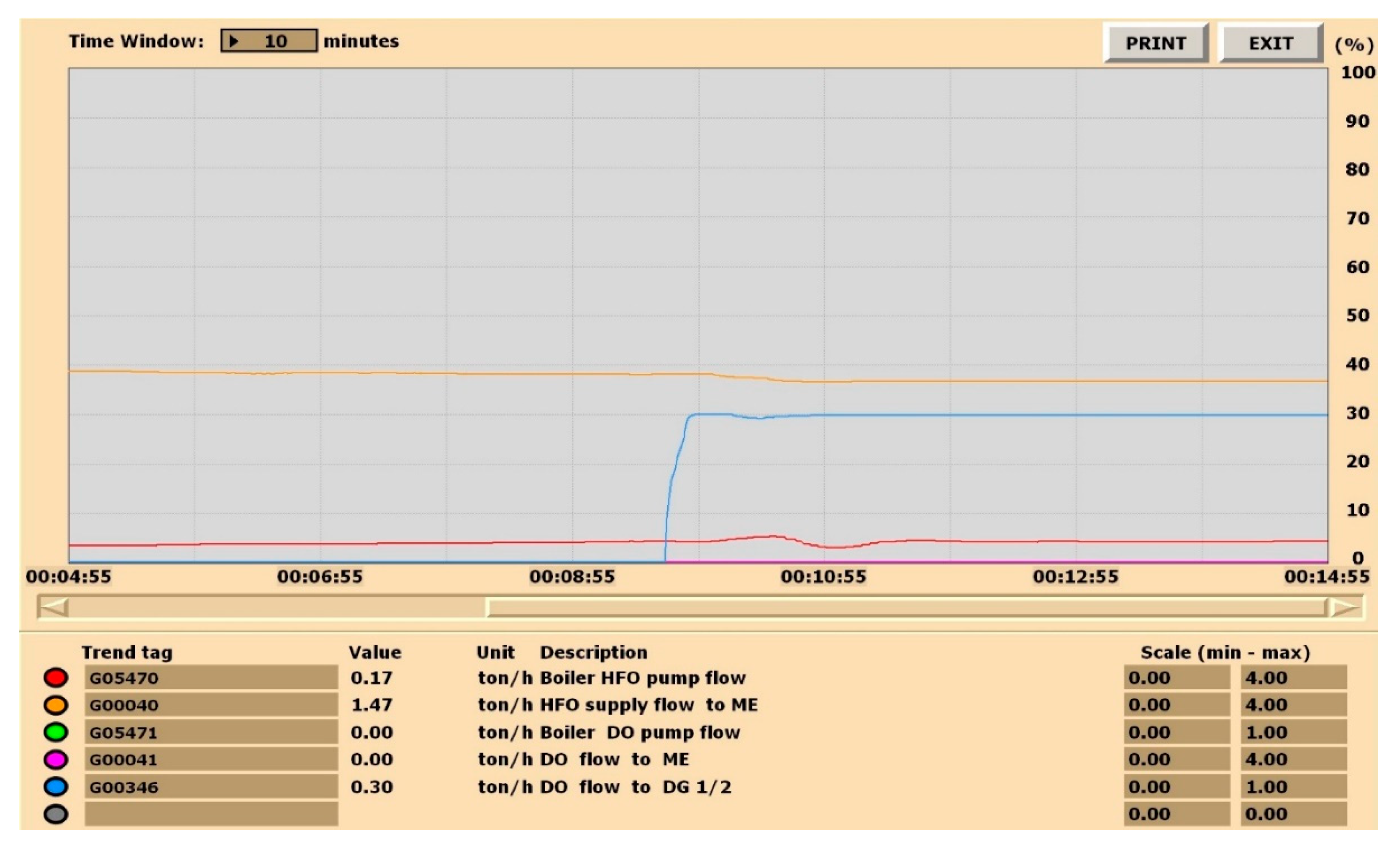
The fuel flow logs for mode 1.3 are shown in
Figure 3. The fuel consumers were: the main engine, one of the electric diesel generators, and the oil-fired boiler. The start of the diesel generator was due to the exhaust reduction in the main engine, which resulted in a power reduction in the TG. After that, the flows remained practically constant.
The fuel flow logs for mode 1.4 are shown in
Figure 4. The only flows were those to the main engine and the oil-fired boiler, and they remained nearly constant throughout the operating period.
The following two figures show the fuel flow logs for the container ship’s engine room and operating modes 2.1 and 2.2, respectively. In operating mode 2.1, the fuel consumption of the main engine and the oil-fired boiler remained constant. The ship speed in operating mode 2.1 was set to full sea speed. Three last flows remained at zero throughout the 200 NM trip.
The time span for the log shown in
Figure 4 was set to 20 min because of some interesting perturbations. As the speed of the ship decreased, the output power of the engine was greatly reduced. Since the speed depended on the power by approximately the third root, there was a corresponding amount of exhaust gas production.
Due to the lack of exhaust gases, the internal combustion engine produced too little steam, and the TG could not produce enough electricity. Since the ship’s power plant was set for optimum operation, no additional steam was produced in the oil-fired boiler unless necessary. The shaft generator was set to AUTO in PTI mode and tried to come online every few minutes. It generated power for the shaft but shut down after a short time because there was not enough power. The highest efficiency of this system was achieved when steam was generated solely by the exhaust generator, there was enough steam for the TG and other auxiliaries, and the TG provided enough power to operate the shaft as a motor. Shutdown of the shaft occurred every few minutes, so in a real situation it would be advisable to turn off the automatic operation (AUTO) mode of the shaft generator.
The first column indicates the modes of operation used: modes 1.1 through 1.4 represent the 5MC90 motor, while modes 2.1 and 2.2 represent the RT-Flex 82C L11 motor. The second, third, and fourth columns indicate the fuel flows to the main engine, boiler, and diesel generators, respectively, measured at the outlet pipes of the service tanks. Travel time was calculated using Equation (2), and vessel speed was taken from the bridge control panel. Btotal is the total fuel consumption, and carbon dioxide emissions were calculated assuming that all the carbon in the fuel had been converted to carbon dioxide.
Carbon dioxide emission was calculated from the data in the seventh column of the
Table 3 (
Btotal), where the mass fraction of carbon was about 83%.
4 This number was multiplied by the coefficient 3.67, which was the increase in the molecular mass of carbon dioxide (44) over the number of carbon atom number (12).
The results were obtained with a simple calculation. The total fuel oil consumption was calculated according to the following formula:
where
BME (t/h) is the fuel oil consumption of the main engine,
Bb (t/h) is the fuel oil consumption of the oil heater,
Bdg (t/h) is the fuel oil consumption of the diesel generator, and
T (h) is the travel time, which was calculated using the expression:
where
S (NM) is the total distance travelled at determined speed, equal to 200 NM, and
V (kn) is the ship’s speed.
In calculating total carbon dioxide emissions (BCO2 [t]), it was assumed that a complete combustion process occurred in all engines or boilers involved—no carbon monoxide or light hydrocarbon fractions were emitted. The approximate mass fraction of carbon in all fuels used during the simulated trip was 85%.
The summary results are shown in the last two columns on the right side of
Table 3, and graphically in
Figure 7 and
Figure 8. For the first engine, the best result (operating mode 1.2) was obtained with the shaft and TG turned on (mode 1.4 had slightly lower efficiency). Fuel consumption and carbon dioxide emissions were reduced by one third in this operating mode. Operating mode 1.3 (with diesel generators switched on) showed lower efficiency in reducing fuel consumption or carbon dioxide emissions. Although power was reduced to 60%, as in modes 1.2 and 1.4, fuel consumption and CO
2 emissions only decreased by about 23%. This was due to the consumption of DGs and the fact that the fuel boiler was on.
The output of the second engine had to be reduced to 40%. Both total fuel consumption and carbon dioxide emissions were reduced by almost half of the original value, but not as much as would be expected if only specific consumption was considered. This was due to the extended travel time.
4. Conclusions
Total fuel consumption and carbon dioxide emission during 200 NM sail at full sea speed, and at speed reduced to 12 knots, were compared. It was expected and confirmed that the lower speed of the VLCC resulted in a significant reduction in fuel oil consumption compared with consumption while travelling at maximum speed. The savings, however, were very different. The two diesel engines we used were significantly different, the second engine being twice as powerful as the first, which made all the difference.
Most previous research has used propulsion engine data only, namely, fuel consumption and carbon dioxide emissions. Our work dealt with all fuel consumers; however, their number, power, efficiency, possible mode of operation, etc., were very different. Although the main engine produced most of the pollutants, pollution from other fuel consumers must also be considered. Our study showed very different results for the same power plant, with ME power reduced to 60% depending on the operation of SG and TG; with their use (modes 1.2 and 1.4), fuel consumption and CO2 emissions were reduced by one third, compared with original values (ME operation at 100% power). Without SG and TG (mode 1.3), the reduction was only 23%.
The savings were greatest when a combination of SG and TG was used. It appears that modern marine power plants, which include shaft generators capable of operating in PTI mode, TG, and other methods of waste heat recovery, achieve the best results at slow speed. In contrast, a classical power plant with a slow-speed main engine and several medium-speed diesel generators showed the worst results.
When the speed of very fast (container) ships is limited to 12 knots, significant fuel consumption and carbon dioxide emissions reductions occur, although the savings are not as high as expected due to the higher specific fuel consumption and longer travel time.
The carbon dioxide reduction measure examined in this paper would have the best impact if applied to modern ships with smart energy saving or waste heat recovery systems. Even then, it seems better to use a power plant management system that works simultaneously with all fuel consumers, instead of a speed limit.
Due to the significant differences in fuel oil consumption and carbon dioxide emissions, and the fact that only a few modes of operation were considered, further studies should follow. These studies should consider different ship loadings, the use of steam to heat liquid cargoes, etc. In addition, emissions of other harmful gases should also be studied.
Since other harmful gases are emitted in addition to carbon dioxide, the question arises as to how the measure under consideration affects their emissions. Perhaps it would be better to determine the total harmful effects. Human history teaches us to be cautious when introducing new, even revolutionary solutions. Some results may not be as positive as expected.


